Deformation Due to Various Sources in a Thermally Conducing Cubic Crystal Material with Reference Temperature Dependent Properties

Leena Rani

I. INTRODUCTION

In anisotropic bodies, it is necessary to study the response of thermally induced disturbances, which may happen during the manufacturing stages. For example, during the curing stages of filament bound bodies, thermal disturbances may be induced by the heat buildup and cooling processes. The level of these disturbances may exceed the ultimate strength of the material. In the last century, a considerable interest is developed in the theory of thermoelasticity that includes such thermal disturbances. After studying the second sound effect in materials as solid helium, bismuth, and sodium fluoride, a systematic research get started.

The classical dynamical coupled theory of thermoelasticity has been extended to generalized thermoelasticity theories by Lord and Shulman (1967) and Green and Lindsay (1972). Dhaliwal and Sherief (1980) extended the generalized theory of thermoelasticity (1967) to anisotropic media. Green and Naghdi (1993) proposed a new theory of thermoelasticity without energy dissipation and presented the derivation of a complete set of governing equations of the linearized version of the theory for homogenous and isotropic materials in terms of displacement and temperature fields.

Chandrasekharaiah (1998) and Tzou (1995) proposed another generalization to coupled theory is known as dual-phase-lag thermoelasticity, in which Fourier law is replaced by an approximation to a modification of the Fourier law with two different translations for the heat flux and temperature gradient. Lin (2004) studied thermoelastic problems in anisotropic half-plane. Kumar and Rani (2007) discussed disturbances due to thermomechanical sources in orthorhombic thermoelastic material. Beom (2013) considered thermoelastic in-plane problems in linear anisotropic solid. Valès et al. (2016) studied determination of heat source dissipation from infrared thermographic measurements. Bockstal and Marin(2017) discussed recovery of a space dependent vector source in anisotropic thermoelastic system. Rani and Singh (2018) studied thermal disturbances in twinned orthotropic thermoelastic material. Zhang et al. (2019) discussed thermo-mechanical coupling analysis of the orthotropic structures by using element-free Galerkin method. Zhou et al. (2020) solved transient heat conduction problems in general anisotropic media and derived three-dimensional Green's functions in bimaterial.

Nowinski (1959,1960,1962) developed thermoelasticity of bodies with temperature dependent properties. Noda (1991) considered thermal stresses in materials with temperature dependent properties. Ezzat et al. (2001) solved a problem of generalized thermoelasticity with two relaxation times in an isotropic elastic medium with temperature-dependent mechanical properties. Othman and Kumar (2009) studied the reflection of magneto-thermoelastic waves with temperature dependent properties in generalized thermoelasticity. Kalkal and Deswal (2014) adopted normal mode technique to investigate the effect of phase lags on three-dimensional wave propagation with temperature-dependent properties. Matysiak et al. (2017) studied temperature and stresses in a thermoelastic half-space with temperature dependent properties. Zhang et al. (2019) studied the effect of temperature dependant material properties on thermoelastic damping in thin beams.

To the best of my knowledge the problem of homogeneous, thermally conducting, cubic crystal material under the effect of dependence of reference temperature on all elastic and thermal parameters has not yet been investigated. In the present problem the component of displacements, stresses and temperature distribution are determined due to mechanical and thermal sources. The solutions are obtained by using Laplace and Fourier technique. The comparison of Linear case, quadratic case and exponential case, respectively, are shown graphically for thermal source for L-S theory.

II. FORMULATION OF THE PROBLEM

We consider a homogenous, thermally conducting cubic crystal, elastic half-space in the undeformed state at uniform temperature $T_{o}$ . The rectangular Cartesian coordinate system $(x,y,z)$ having origin on the plane surface z=0 with z-axis pointing vertically into medium is introduced. A concentrated and uniformly distributed mechanical or thermal source is assumed to be acting at the origin of the rectangular Cartesian co-ordinates. Here we consider plane strain problem parallel to xz-plane with displacement vector $\vec{u}=(u,0,w)$ and temperature $T(x,z,t)$ , then the field equations and constitutive relations for such a medium in the absence of body forces and heat sources can be written, by following the equations given by Lord-Shulman (1967), Green and Lindsay (1972) and Dhaliwal and Sherief (1980) as

and

where

and $c_{ij}$ are isothermal elastic parameters, $\rho, c_{e}$ and $\tau_{0}, \tau_{1}$ are, respectively, the density, specific heat at constant strain and thermal relaxation times. $\alpha$ is the coefficient of thermal expansion, $\delta_{1k}, \delta_{2k}$ are Kronecker deltas, K is the coefficient of thermal conductivity. u and w are displacement components along x and z directions respectively, t is time, T is temperature change, $t_{zx}$ and $t_{zz}$ are stresses. Lord-Shulman (L-S) theory, $t_{1} = \tau_{1} = 0$ , $\tau_{0} > 0$ , k = 1, $n^{*} = n_{o} = n_{1} = 1$ , and for Green and Lindsay (G-L) theory, $t_{1} = 0$ , $\tau_{1} \geq \tau_{0} > 0$ , $n_{o} = 0$ , $n^{*} = n_{1} = 1$ . For Green and Naghdi theory (G-N) (type II) $n^{*} > 0$ , $n_{1} = 0$ , $n_{o} = 1$ , $t_{1} = \tau_{1} = 0$ , $\tau_{0} = 1$ . where $n^{*} = constant$ has the dimension of [1/s], and $n^{*} K = K^{*} = c_{e} c_{11}/4$ is a characteristic constant this theory.

For Chandrasekharaiah and Tzou (CTU) theory is such a modification of classical thermoelasticity model in which Fourier law is replaced by an approximation of the equation

where $q_{i}$ is the heat flux vector. The model transmits thermoelastic disturbances in a wave like manner (1986) if Eq. (4a) is approximated by

where $0 \leq \tau_{\theta} < \tau_{q}$ . and $t_1 = \tau_{\theta} > 0$ and $\tau_{\theta} = \tau_{q} > 0$ , $n^{*} = n_{o} = n_{1} = 1$ , $0 \leq \tau_{\theta} < \tau_{q}$ , $\tau_{1} = 0$ . $\mathsf{c}_{ijkl}$ satisfies the (Green) symmetry conditions:

The initial and regularity conditions are given by

For dependency of all elastic and thermal parameters on reference temperature we have taken three cases (i) Linear case (ii) quadratic case (iii) Exponential case The material constants are given as (2016, 2001) For Linear case

For quadratic case

For exponential case

where $c_{ij0}, \beta_{0}, K_{0}, v_{0}, c_{e0}$ are considered as constants, $\alpha^{*}$ is called empirical material constant. In case of the system independent of reference temperature, $\alpha^{*}=0$ .

III. SOLUTION OF THE PROBLEM

We introduce dimensionless quantities as

where $v_{1}=\left(\frac{c_{110}}{\rho}\right)^{\frac{1}{2}}$ and $\omega_{1}^{*}=\frac{c_{e0}c_{110}}{K_{0}}$ are, respectively, the velocity of compressional waves in x-direction and characteristic frequency of the medium.

Equations (1)-(3) with the help of equations (7)-(9), can be written in non-dimensional form as (dropping the dashes for convenience)

For linear case $\mathrm{A}^{*} = \frac{1}{(1 - \alpha^{*}\mathrm{T}_{0})}$ , for quadratic case $\mathrm{A}^{*} = \frac{1}{(1 - \alpha^{*}\mathrm{T}_{0})^{2}}$

and for exponential case $A^{*}=\frac{1}{e^{\alpha^{*}T_{0}}}$

Applying the Laplace and Fourier transforms

on equations (12) - (14) and eliminating $\widetilde{\mathbf{u}},\widetilde{\mathbf{w}},\widetilde{\mathbf{T}}$ from the resulting expressions, we obtain

where

The roots of Eq. (16) are $\pm \lambda_{\mathrm{i}}$ ( $i = 1,2,3$ ). Using regularity condition (6), the solutions of Eq. (16) may be written as

with $\mathrm{A}_{\ell}(\ell = 1,2,3)$ being arbitrary constants.

IV. APPLICATION

a) Instantaneous Load

i. Mechanical boundary conditions

where $\delta(t)$ is the Dirac's delta function and $\psi(x), \zeta(x)$ specify the vertical and horizontal source distribution functions, respectively, along x-axis. h is heat transfer coefficient.

Using equations (4),(10)-(11),(15), in the boundary conditions given by Eq. (20) and with the help of Eqs. (17) - (19), we obtain the expressions for displacement components, stresses and temperature distribution as

p_n = \frac{1}{\rho v_1^2} \left(-i\xi c_{12} + c_{110} a_n b_n\right) - \beta b_n \left(1 + p\tau_1 \delta_{2k}\right),\(n=1,2,3).

Case I: Concentrated Force In this case, we take

in equation (20).

Using the Laplace and Fourier transforms defined by equations (15) in equation (22), we get

where $\delta (x)$ is the Dirac delta function having the property

Case II: Uniformly Distributed Force

The solution due to uniformly distributed force applied on the half-space surface is obtained by setting

in equation (20). Taking Laplace and Fourier transforms with respect to the pair $(\mathbf{x},\xi)$ , we obtain

The expressions for displacement components, stresses and temperature distribution are obtained for concentrated force, and uniformly distributed force by replacing $\widetilde{\psi}(\xi),\widetilde{\zeta}(\xi)$ from equations (23),(25) respectively, in equation (20).

b) Thermal boundary conditions

$\frac{\partial\mathrm{T}}{\partial\mathrm{z}} = \eta (\mathrm{x})\delta (\mathrm{t})$ at $z = 0$ , for the temperature gradient boundary, or

$T = \eta(x)\delta(t)$ at z = 0, for the temperature input boundary,. (26)

Using equations (4), (10)-(11),(15), in the boundary conditions given by Eq. (26) and with the help of Eqs. (17) - (19), we obtain the expressions for displacement components, stresses and temperature distribution as

On replacing $\Delta$ by $(\mathrm{T}_{0}\omega_{1}/\mathrm{v}_{1})\Delta_{1}^{*}$ and $T_{0}\Delta_{2}^{*}$ in Eq. (27), we obtain the expressions for temperature gradient boundary and temperature input boundary, respectively.

For temperature gradient boundary we replace and for temperature input boundary we take in Eq. (27).

Case I: Thermal Point Source In this case

with

Case II: Uniformly Distributed Thermal Source Here

with

Replacing $\widetilde{\eta} (\xi)$ from equations (28)-(29) in equation (27), we obtain the corresponding expressions for thermal point source and uniformly distributed thermal source, respectively.

c) Continuous Load

i. Mechanical sources on the surface of half-space The boundary conditions in this case are

where $H(t)$ is the Heaviside unit step function, P is the magnitude of the force, $\psi(x)$ , $\zeta(x)$ specify the vertical and horizontal source distribution functions, respectively, along x-axis. h is heat transfer coefficient.

Adopting the same procedure of previous section (4.1a), using the boundary conditions (30), replacing $\Delta_{\ell}(\ell=1,2,3.....,8)$ with $\frac{\Delta_{\ell}}{p}(\ell=1,2,3.....,8)$ , respectively, in equation (21), we obtain the corresponding expressions for the components of displacement, stresses and temperature distribution.

The corresponding expressions for concentrated force and uniformly distributed force are obtained by replacing $\widetilde{\psi}(\xi),\widetilde{\zeta}(\xi)$ and $\Delta_{\ell}(\ell=1,2,3,\ldots,8)$ with $\frac{\Delta_{\ell}}{p}(\ell=1,2,3,\ldots,8)$ , from equations (23), (25) in equation (21), respectively.

ii. Thermoelastic Interactions due to Thermal Source The boundary conditions in this case are

$\frac{\partial\mathrm{T}}{\partial\mathbf{z}} (\mathrm{x},\mathrm{z} = 0) = \eta (\mathrm{x})\mathrm{H(t)}$ , for the temperature gradient boundary, or

Adopting the same procedure of previous section (4.1b), using the boundary conditions (31) and replacing $\Delta'(\ell = 1,2,3\ldots,8)$ with $\frac{\Delta'}{p} (\ell = 1,2,3\ldots,8)$ , respectively, in equation (27), we obtain the corresponding expressions for the components of displacement, stresses and temperature distribution.

Replacing $\widetilde{\eta} (\xi)$ from equations (28)-(29), in equation (27) we obtain the corresponding expressions for thermal point source and uniformly distributed thermal source respectively.

Sub-case 1: If $\mathrm{h} \to 0$ , Eq. (21) yield the considered variables for the insulated boundary.

Sub-case 2: If $\mathrm{h} \to \infty$ , Eq. (21) yield considered variables for the isothermal boundary.

Particular Case

Taking

we obtain the corresponding expressions for the isotropic thermoelastic material.

V. INVERSION OF THE TRANSFORMS

To obtain the solution of the problem in the physical domain, we must invert the transformed equations (21) and (27), for the four theories, i.e., L-S, G-L, G-N and CHT by using the method of inversion described by Kumar and Rani(2007).

VI. NUMERICAL RESULT AND DISCUSSION

Following Dhaliwal and Singh (1980), we take the case of magnesium crystal-like material for numerical calculations. The physical constants used are:

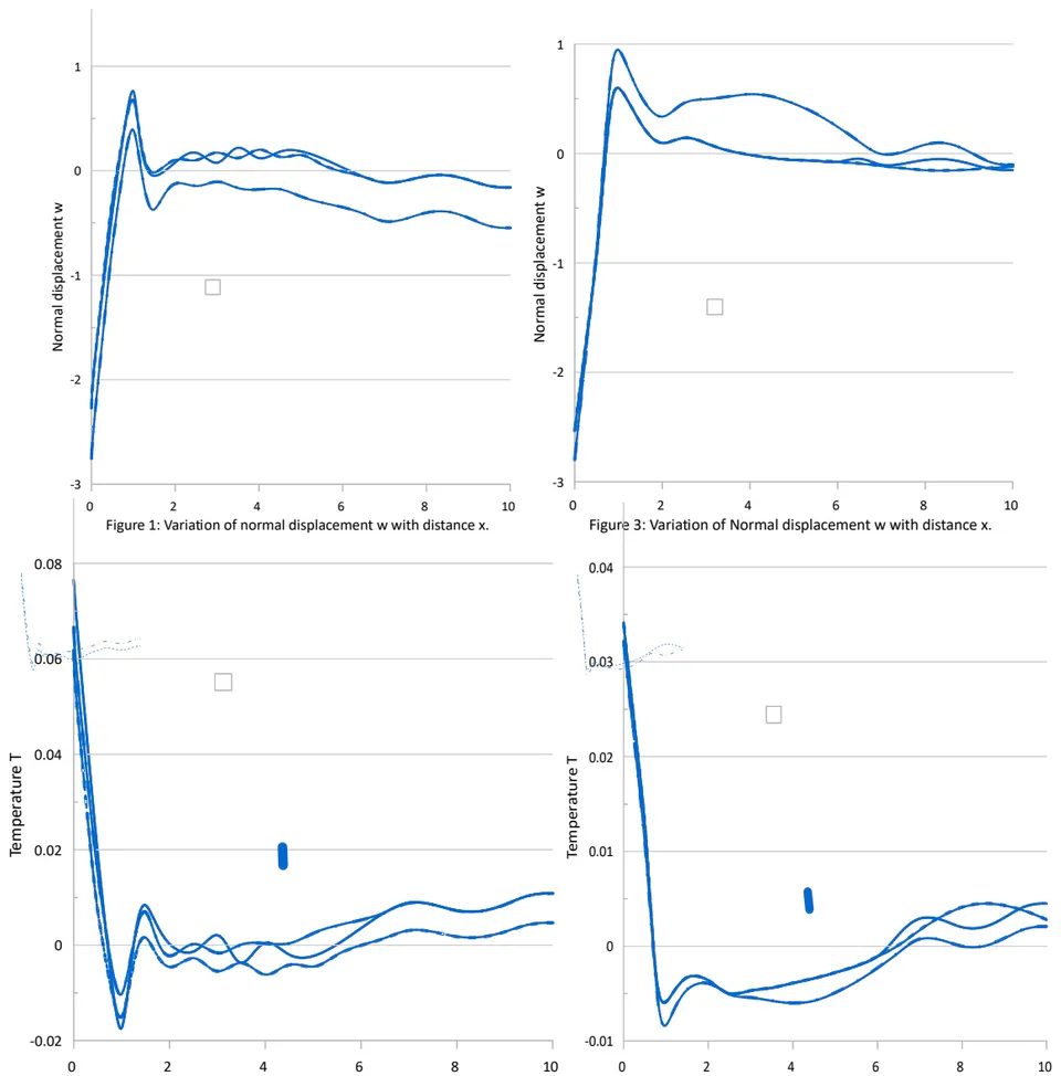
The variations of normal boundary displacement $w$ and boundary temperature field $T$ with distance $x$ at non-dimensional time $t = 1.0$ are shown graphically in figures 1-4, for L-S, for non-dimensional relaxation times $\tau_0 = 0.02$ . The computations were carried out for time $t = 1.0$ and $\alpha^* = 0.00051$ at $z = 1.0$ in the range $0 \leq x \leq 10$ . The solid lines (——), the small dashed lines (-----) and the long dashed lines (---), in graphs represent the variations for Linear case, quadratic case and exponential case, respectively for L-S theory. The results for distributed thermal source are presented for dimensionless width $a = 1$ . The figures (1)-(4) are depicted for thermal source.

a) Instantaneous Load

i. Thermal source on the surface of half-space (Temperature gradient boundary)

a. Thermal point source

Figure 1. shows the variation of normal displacement 'w' with distance x. The values of normal displacement starts with sharp increase and then become oscillatory in the whole range for Linear case, quadratic case and exponential case. The values of normal displacement for linear and quadratic case are more than the exponential case in the whole range $0 \leq x \leq 10$ .

Figure 2. depicts the variation of temperature distribution T with distance x. Initially the values of T start with sharp decrease and then become oscillatory about zero in the whole range for Linear case, quadratic case and exponential case. The values of 'T' shows appreciable effect for all the three cases.

b. Uniformly Distributed Thermal Source

Figure 3. depicts the variation of normal displacement w with distance x. The values of normal displacement in all the three cases start with sharp increase, the values show very small variation about zero in the whole range for linear and quadratic case. The values of normal displacement for exponential case are more than linear and quadratic case in the range $0 \leq x \leq 10$ , which shows the appreciable effect of exponential case.

Figure 4. depicts the variation of temperature distribution T with distance x. At the point of application of source, the values of T decrease sharply for all the three cases. The values of T for linear and quadratic case are more than exponential case in the range $0.5 \leq x \leq 6$ . In range $6 \leq x \leq 10$ , the values of 'T' for quadratic case shows opposite oscillatory pattern in comparison to linear and exponential case.

VII. CONCLUSION

The comparison of linear and quadratic and exponential case has been depicted for L-S theory for temperature gradient boundary.
As 'x' diverse from the point of application of source the components of normal displacement and temperature are observed to follow small variations about zero in the range $1 \leq x \leq 10$ for instantaneous load.
The variations of normal displacement and temperature distribution for uniformly distributed thermal source are same as those of Thermal point source with difference in their magnitude for all the three cases.

Figure 2: Variation of Temperature T with distance x. Figure 4: Variation of Temperature T with distance x.