

I. INTRODUCTION
For thousands of years human beings have used the power of flowing water for various activities. Ancient civilizations used wooden paddle wheels to grind wheat and corn into flour. Hydro means Water in Greek, the word hydropower traditionally represents the energy generated by damming a river and using turbine systems to generate electrical power (Westra, 2008). However, there are several other ways we can generate energy using the power of water. Ocean waves, tidal currents and ocean water temperature differences can all be harnessed to generate energy.
Due to the depletion of natural resources and the global environmental problems, there is an international call for the need to develop renewable energy sources which have minimal environmental impact. Out of all the renewable energy resources one of the most mature techniques for renewable power generation is hydro-electric power. Large numbers of hydroelectric power generation plants are found in various countries of the world and the technology is now quite mature (Karassik et.al, 2008). However, considering the benefit from the economics of scale the possibility of implementing a policy of building large scale hydroelectric power generation plants is not always technologically, economically and environmentally feasible (Westra, 2008). Consequently, the interest in small scale hydroelectric power generation is increasing in most part of the developing countries of the world. In most cases construction costs for such plant are relatively high when compared with the small amount of power generation they produce (Tanbhir et al.). The high cost of construction limits the possibility for its proper implementation. If the cost of construction could be decreased small scale hydroelectric power production could become the more preferred renewable energy scheme the world over, most especially in the third world.
It is a well-known fact that electrical energy allows people to have better living conditions. Unfortunately in Nigeria there are still isolated places without the possibility of acquiring this all important resource. Some rural areas that are still not connected to the national grid exposes an opportunity where solutions could be found using pumps as turbines as an option or alternative to solving the electrical energy need.
For very low hydroelectric power plants (power less than 100 kW), the possibility of using pumps instead of turbines deserves optimum consideration which could be used for stand-alone or duel electricity generation purposes, even though there is an efficiency drop, a significant reduction in the capital cost of the plant gives it an advantage of the order of 10 to 1 or even more (Singh, 2005). The reverse working mode of a centrifugal pump is now being investigated and the technology for their use in electrical power generation is now scantily available. The advancement in electrical machinery control technologies, that allows the driving regulation with variable velocity, rotation sense and torque has created the possibility of the utilization of pumps working in inverse mode for power generation (He Zheng, 2011).
All known conventional turbines have inlet guide vane but a centrifugal pump working in reverse mode does not have one, This makes the variable discharge characteristic slightly different from that of common turbines (Mohd Azlan et al.). However, the reverse running mode of a centrifugal pump has the advantage of uniform quality, simple construction and durability. A reverse running pump turbine also has almost same efficiency as the pump, which is competitive with other turbine types; a small number of parts enable easy maintenance and inspection. (Fernandez, et al 2004).
This work examined the characteristics of a specific pump acting in inverse mode against rotational speed. To accomplish this, a suitable facility has been designed, built and characterized.
II. MATERIALS AND METHODS
a) Materials
The following are the materials and instruments that were used and selected for the experiment: two centrifugal pumps, PVC pipes, PVC sockets, PVC elbows, PVC gum, thread seal tape, a galvanized iron tank, nuts, bolts, belt, sole blade and gauge valves. A large PVC ground tank, an overhead galvanized iron tank, a tachometer and a manometer. Some iron flat bars were used to repair and support the galvanized iron tank.
| S/N | Material/Instruments | Pump Specification | Turbine Specification |
| 1 | Centrifugal Pump | 3.8 hp | 3.8 hp |
| 2 | Gauge Valve | 51 mm | 79 mm |
| 3 | Intake Pipe | Diameter 51 mm | Diameter 79 mm |
| 4 | Out Pipe | Diameter 65 mm | Diameter 68 |
| 5 | Ground Tank | As Adequate | As Adequate |
| 6 | Tachometer | Cyber Tech. (NUSPSC 25174406) | Cyber Tech. (NUSPSC 25174406) |
| 7 | Manometer | Canstock (csp 14719981) | Canstock (csp 14719981) |
| 8 | Stop Watch | Digital | Digital |
| 9 | Impeller | Open Type | Pelton Type |
b) Methods
i. Performance Test on the Pump
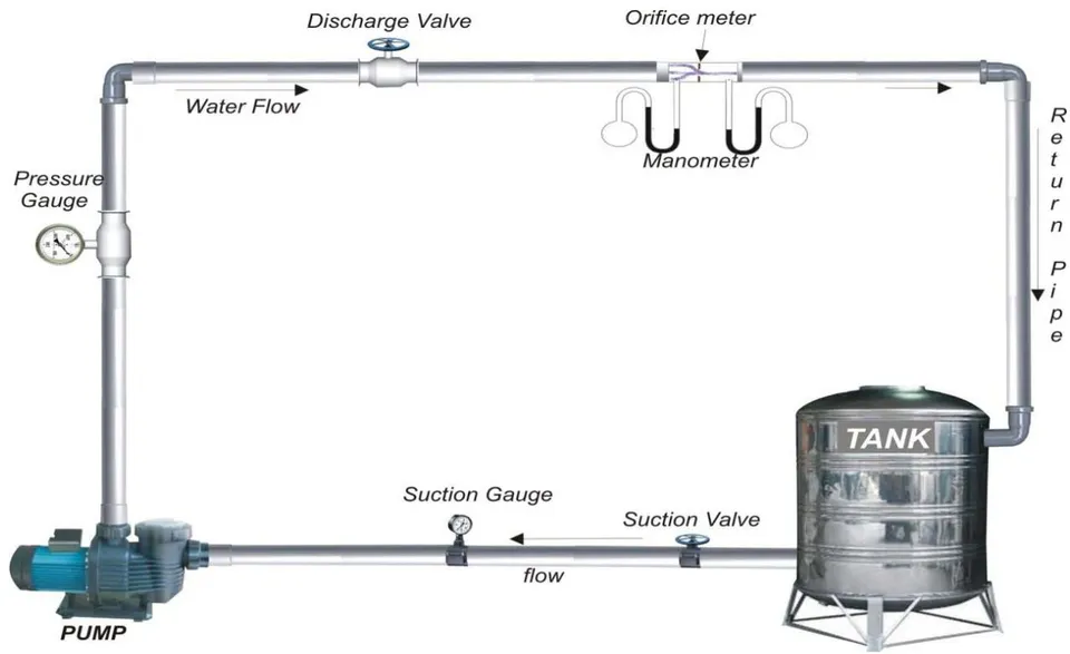
For the experimental set-up on the test performance of the pump a (m) centrifugal pump was used and connected to a motor. The schematic diagram (Fig.1) illustrates the experimental set up of the pump and motor test. Connected to the pump and motor are the inlet pipe, the discharge pipe, the Orifice meter, the tank and various instruments that were used for the measurements.
The centrifugal pump was connected to three (3) inch pipes coupled with delivery and discharge valves which were used to vary the flow rate of water as desired. The manometer and orifice meter were used to measure the pressure on the pump discharge head, while the tachometer was used to measure the speed of the pump at different flow rate by placing it at the extreme end of the shaft of the engine. A digital stop watch was used as the timing device to measure the time of the rotation of the engine in revolution per minute at an interval of twenty minutes (20 min). This was done to take record of the pump speed and the pressure difference.
Three moderate size local calabashes were placed on the top of the water in the tank so as to reduce turbulence while the test experiment was on going. The water retunes back to the tank and the water recycling was continued until all measurements were concluded. This process was repeated six times and readings were equally taken for time the process was repeated.
ii. Centrifugal Pump Test
a. Determination of Flow Rate (Q)
Using the process adopted by Thapar (1984) and Boys (1987) the flow rate was determined. See equation (2.1)
Q is the flow rate in liter/second and
pressure differential in cm Hg
b. Determination of Power Input
- Measuring and Calculating Power Input( ) - Fuel (Petrol) Rate ( ) of Consumption To measure the rate of fuel (petrol) consumption for running and testing the Centrifugal pump in pump mode which is the power input of the pump, the method adopted by Henggeler et. al. (2005) was used.
This Volumetric method can be used to calculate Petrol rate which in turn is also the power input by measuring the gross changes in bulk volume over a longer period of time. This is done by calculating the amount of petrol used by the centrifugal pump during a set duration of one hour (60 minutes)
This is achieved by dipping the current surface level of the petrol inside the tank with a clean meter rule, the level is marked and recorded. After doing this the centrifugal pump was switched on and immediately the stop watch was started. The centrifugal pump was allowed to run for one hour at a particular speed (rpm). The flow rate was than measured. This procedure was repeated six different times at different speed (rpm). After the end of every hour of running the test the meter rule was dipped inside the tank of the centrifugal pump and the new level was marked and recorded both on the meter rule and on the tank. Noting that the tank of the centrifugal pump which is always cubic shaped without graduated markings, there was a need to calculate the liter of petrol inside the tank based on tank length, diameter and the depth of fuel surface.
The volume of petrol in liter inside the tank of the centrifugal pump at any instance is given by,
The quantity of petrol used during the time period is then the difference in liters as determined by equation (2.3) calculated at the end of the period versus what it was at the start of the period. To turn these volumetric amounts into Petrol consumption rate the difference in volume was divided by the additional clocked hours on the gauge that was first marked down from the original amount. Equation (2.3) calculates the petrol consumption rate for this period. (Henggeler et.al. 2005)
iii. Determination of Speed
The speed was measured (in rpm) with an optical electronic hand held tachometer. The tachometer was placed at the end of the pump shaft so the reading could be taken accurately.
iv. Determination of Power Output
The method of Henggeler et. al. (2005) to calculate the power output of the centrifugal pump in pump mode test was adopted. The generated water horsepower was used as the power output . It was calculated from equation 2.4
v. Determination of Pressure
A manometer and orifice meter was used to measure the pressure. They were mounted on the discharge pipe few distance away from each other and the readings was recorded.
vi. Determination of Efficiency
The process used by Raman et al. (2013) was adopted to determine the pump efficiency. From equation 2.5
- Effect of Speed on Efficiency of the Pump
The variation of the pump speed with its efficiency is shown in Figure 3.1. This shows the measure of the effectiveness of a machine in transferring energy and power expressed by the ratio of the device's output per its input. (Nautiyal et al. 2011).
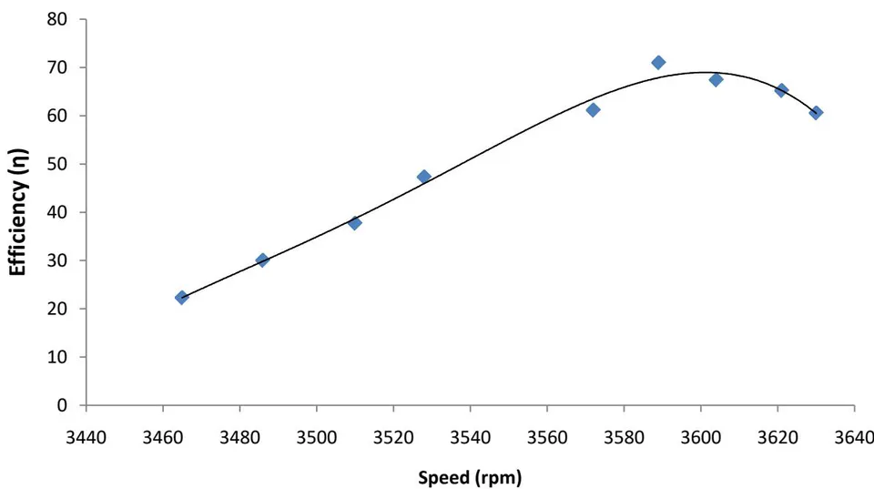
Figure 3.1 is a curvilinear and portrays the fact that as speed of the pump increases the efficiency of the pump also increases, at the maximum speed at which the pump was run (3589 rpm), the best efficiency point (BEP) of the pump was . This is the point at which the pump gave its best performance. Jose (2010) obtained much lower efficiency 44% possibly due to hydraulic losses associated with the type of centrifugal pump he used.
The regression analysis shows that the P-value is 0.000012, (Table 17 Appendix C), indicating the model is significant at 95% confidence level. From the coefficients, the efficiency increased by 0.385 for every one point increase in the speed (Equation 3.1). With value of 0.9919, the model (Equation 3.1) is a good fit to the data.;
c) Effect of Efficiency on Flow Rate (Pump)
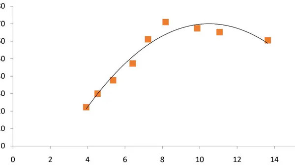
Figure 3.2 portrays the variation of efficiency with flow rate. From Figure 3.2, it is clear that the higher the flow rate, the higher the efficiency of the pump as reported in the literature (Fernandez et al. 2004).
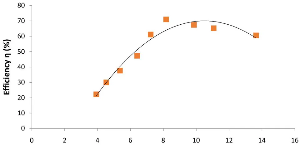
The maximum flow rate of the pump mode was because increasing flow rate during pump mode test led to lower pressure of the fluid at the suction part of the pump which caused formation of bubbles and thereby allowed cavitation in the pump as observed by Teuteberg (2010) and Nautiyal et al. (2011). From the regression analysis, (appendix Table 18), value is 0.9564, which shows a good fit to the data as of the experimental data is explained by the model (Equation 3.2). The P-value is it is significant and has a good relation between flow rate and efficiency. For the coefficient; the efficiency increases by for every one point increase in power input. The intercept is .
d) Effect of the pump Fuel Consumption on Efficiency
Figure 3.3 portrays the variation of efficiency with fuel level. It shows clearly that as the speed (rpm) of the pump increases the flow rate also increases causing the rate of fuel consumption to increase thereby bringing about increased drop in the fuel level in the tank of the centrifugal pump.
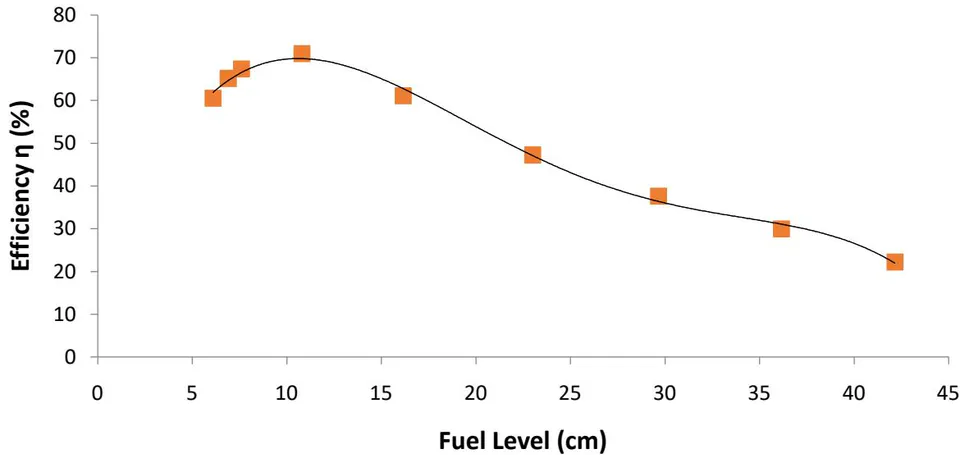
Figure 3.3 also indicates a trend curve that shows that the efficiency is indirectly proportional to the level of fuel in the tank. This agrees with Henggeler et al. (2005).
In the regression analysis (appendix Table 19), P-value is 0.00000122, this indicates the significance of the model at a confidence level of 96%. From the coefficient; the efficiency decreased by -1.487 for every one point increase in fuel level (Equation 3.3). The value is 0.993, the model (Equation 3.3) is a good fit to the data.
e) Effect of Efficiency on Pump Power Input
Figure 3.4 portrays the variation of efficiency with Power input. Figure 3.4 demonstrates that efficiency was increasing as the power input was also increasing. This result agrees with the work of Westra (2008) and Raman and Hussein (2009).
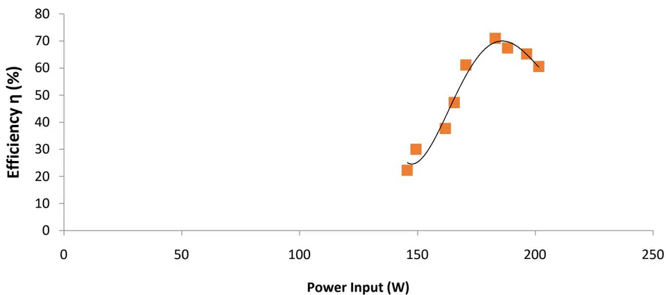
At the maximum efficiency of , the power input was 180W, and at the minimum efficiency of the power input was . This result also agrees with that of Rusovs (2002) and Westra (2008).
From the regression analysis (appendix Table 20), value of 0.9701, shows a good fit of the model (Equation 3.4) to the data. It shows that of the experimental data is explained by the model (Equation 3.4). The P-value of shows that the model in accounting for the experimental data is significant. From the coefficient; the efficiency increases by for every 1W increase in power input.
f) Effect of Power Output on the Pump Efficiency
Figure 5 shows that the efficiency is directly proportional to the pump power output. At the peak power output of 129.91W, the efficiency of the pump was .
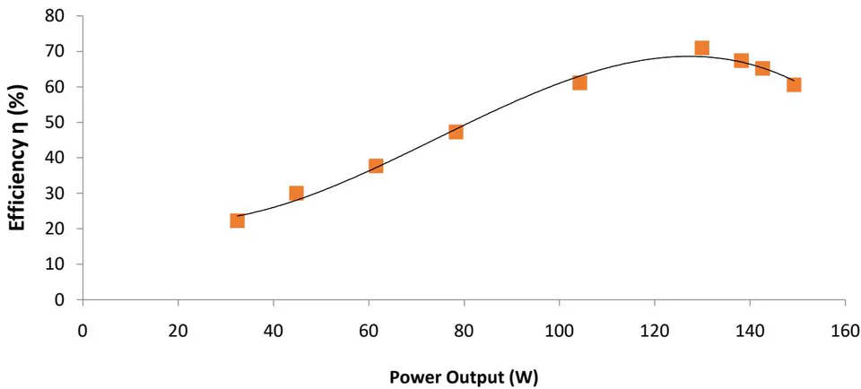
This characteristic curve proves that the higher the fluid discharge rate the higher the power output and this gives a corresponding better efficiency of the pump. This result agrees with that reported by Nuatiyal et al. (2011) and Teuteberg (2010).
From the regression analysis (appendix Table 21), value is 0.9929, which shows a good fit to the data as of the experimental data is explained by the model (Equation 3.5). The P-value is 0·00607 it is significant and has a good relation between power output and efficiency. From the coefficient; the efficiency increases by 0·5047 for every one point increase in the power output.
g) Effect of Flow Rate on Power Output (Pump)
Figure 3.6 shows that the power generated is proportion to the flow rate, in agreement with the result obtained by Raman et al. (2013).
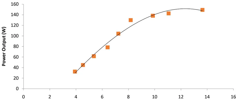
Six different flow rate values were used to obtain flow characteristics in the test pump. The flow rate was changed from to different speed (rpm) of the pump. The optimal rate of flow was which was the peak since the graph gave a curvilinear (Figure 3.6). Figures 3.2, 3.3 and 3.6, show that the characteristic curves from this work are in conformity with the results obtained by Raman and Hussein (2009).