
Chapter 1
Introduction
Background of the study
Agriculture sector employs 80% of the population of Rwanda and contributes 33% of GDP growth. Agriculture is the backbone and key component of Rwanda’s fast growing economy. In recent years, the sector has gained significant growth from 4.5% to 6% per annum and is gradually shifting from subsistence to a market-oriented model (RDB, 2020). According to the research conducted by Habineza, Nsengiyumva, Ruzigamanzi, and Nsanzumukiza (2020),(Habineza and Al 2020) the study conducted by (Postel, Polak, Gonzales, & Keller, 2001); RAO (2018), Irrigation contributes to agricultural growth and reduces poverty directly through permitting intensification and di-versification, hence increased outputs and incomes; increasing agricultural wage employment; and reducing local food prices. Irrigation has contributed significantly to poverty alleviation, food security, and improving the quality of life for rural populations. In addition, the developed by Rwanda (2018), there is overall 4% of areas are irrigated in season A. There is no irrigation for crops in hillside and rangeland areas and they reported that there is 26% irrigation in marshland. The highest irrigation of 19% was found in Huye district and 18% in Rusizi districts.
Rwanda has abundant water resources, they are not evenly distributed. Rainfall is high in the western part of the country and low in the east. The issue of variability is critical for lands on hillsides where water cannot be retained. Farms in the eastern part of the country, where rainfall is lowest, are therefore the most vulnerable. With reference to surface water bodies, the eastern part of Rwanda has abundant rivers and lakes that could be harnessed for irrigation purposes. For ground water resources, central and eastern parts of the country indicate good potential especially for springs and borehole development (Solomon & Quiel, 2006). Currently, the most commonly used method is flood irrigation in the marshlands. Plans are afoot to set up demonstration farms in drought-prone eastern Rwanda to educate farmers about the advantages of irrigation. The importance of the role of irrigated agriculture in achieving food security and offering a way out of poverty is not in question. Where irrigation has been introduced, doubling of yields is commonly achieved (Solomon & Quiel, 2006).
Drip irrigation figures prominently in proposed solutions to the water crisis. In national and international policy documents, it is seen and promoted as a device to use water more efficiently (RAO, 2018; Van der Kooij, Zwarteveen, Boesveld, & Kuper, 2013). The belief in the water saving potential of drip irrigation is often substantiated with impressive statistics and measurements. The study conducted by (Postel et al., 2001); RAO (2018) for instance claims that drip irrigation has the potential to at least double crop yield per unit water in many applications, including irrigation of most vegetables, cotton, sugarcane, and orchard and vineyard crops. A collection of research results from various Indian research institutes indicates typical water use reductions with drip irrigation of 30–60% and typical yield increases of 20–50% for a variety of crops, including cotton, sugarcane, grapes, tomatoes, and bananas (Postel et al., 2001). Together, the greater water application efficiency and higher yields produce a doubling or tripling of water productivity” (Postel et al., 2001). Likewise, in an article in Nature, Van der Kooij et al. (2013) asserts that “Shifting from conventional surface irrigation to drip irrigation in India has increased overall water productivity by 42–255% for crops as diverse as banana, cotton, sugar cane and sweet potato”. Numbers like those mentioned by (Klaver, 2003)circulate widely in irrigation and water policy reports, underscoring that drip irrigation is a promising technology to help solve the water crisis. Reports also often contrast drip irrigation with surface irrigation methods, which are presented as inefficient and using excessive amounts of water. A World Bank report for instance states: “Drip irrigation uses 30–50% less water than surface irrigation, reduces salinization and waterlogging, and achieves up to 95% irrigation efficiency” (Van der Kooij et al., 2013).
Problem statement
Dry farming systems depend on precipitation, specifically the component called green water, which is stored directly in the soil and used later as evapotranspiration. In water scarce regions, green water resources make up 85% to 90% of the precipitation, reflecting the significant proportion of the available freshwater that sustains rain fed agriculture. According to IWMI, (2007) due to lack of water storage and large spatial and temporal variations in rainfall, there is not enough water for most farmers to produce more than one time per year and also there are frequent crop failures due to dry spells and droughts which has resulted in a chronic food shortage currently facing the country. Development agencies have tried to encourage farmers to adopt treadle pumps, pitcher pot systems, micro-irrigation systems, water harvesting techniques and a host of other technologies with mixed success. While it may be that some of the technologies simply did not perform up to the expectations, there is a natural tendency to over-emphasize the technology itself rather than pay attention to the process by which it is identified, modified, and disseminated. Currently, Rwanda is promoting horticultural crops farming through advanced irrigation technology adoption to increase the volume of export on the international markets. Actually, there is no specific study conducted in Rwanda to assess the performance evaluation of drip irrigation system on carrot production. Hence, the research focused the analysis of weather parameters, study of soil properties like physical properties pertaining to bulk density, porosity, infiltration rate etc. There is a need to study the uniformity coefficient and application uniformity of water under drip irrigation system to understand the best use of water; hence this study is taking up in IPRC Gishari farm to close the knowledge gap.
Objectives of the study
Overall objective
The overall objective of the study is the performance evaluation of drip irrigation system on carrot production at IPRC Gishari farm in Rwanda.
Specific objectives
The following specific objectives are formulated to reach the overall objective.
To determine weather parameters of the experimental site
To determine the soil properties at the experimental site
To determine water requirement, water deficit and irrigation scheduling of carrot using CROPWAT 8.0
To assess the uniformity coefficient of water under drip irrigation system
To assess the yield of carrot under drip irrigation in experimental plots
Research questions
The various research questions that will be answered at the end of the research work are given below
What are the weather characteristics of the IPRC Gishari farm?
What are the soil physical properties at IPRC Gishari farm?
What will be the crop water requirement, water deficit and drip irrigation schedule of carrot crop?
What is the uniformity coefficient of water for carrot crop under drip irrigation system?
What is the yield of carrot under drip irrigation system in the experimental plots?
Scope and limitation of this research
The present research is to meet the partial requirement of getting master degree in Soil and Water Engineering. It is a student research project. The scope of the research is the performance evaluation of drip irrigation on carrot production. The effect of weather parameters, soil properties. It is intended to study also the crop water requirement and irrigation schedule of carrot will be studied using CROPWAT 8.0 software. There is a need to study also the uniformity coefficient and application uniformity of water for carrot crop will be found out and finally to study the yield of carrot under drip irrigation system will be experimentally found out from the field experiment.
Significance of the study
Soil characteristics from IPRC Gishari farm seems to have the physical and chemical properties in nature. In the same vein of understanding various causes of low horticultural crop productivity in the area, it is similarly important to be focused on sustainability assessment of soil in terms of physical and chemical properties and their effects on horticultural crops. This study is useful to shed light on the performance of drip irrigation on carrot crops in the area. There is a need to scale up productivity and improve quality to meet the country’s strategic goals of improving export earnings and producing adequate quantities for fresh consumption and processing at home level. Furthermore, this study is useful on the scientific level because it will act as reference material for further researchers for higher learning institutions; it will also help the policy makers and implementers to formulate appropriate strategies to improve the drip irrigation system more efficiently and soil properties to boost the crop productivity with the positive influence on smallholder farmer’s livelihood in Rwanda.
Thesis Outline
The study is organized into five chapters. The first chapter gives a general background of the study where among other things; it presents the problem statement, study objectives and research questions. The second chapter gives a literature review related to weather parameters of the experimental site, soil properties at the experimental site, water requirement and irrigation scheduling of carrot using CROPWAT, to study the uniformity coefficient and application uniformity of water, and the literature review on the yield of carrot under drip irrigation. Meanwhile the third chapter gives a detailed description of the materials and methods employed for this study not only site description but also statistical analysis. The fourth chapter presents results and discussion and the last chapter provides the conclusions and recommendations of the study.
Chapter 2
Literature review
Introduction
This present research has been taking into reflection by reviewing diverse related literatures and papers presented in various workshops and seminars, technical reports, text books and browsing through concerned websites. Literatures of review considered a number of subjects including weather parameters on crop production, soil properties (Physical and chemical properties), water requirement and irrigation scheduling, uniformity coefficient and application uniformity of water and thereafter come up with estimation of yield of carrot under drip irrigation. This chapter is organized as follows:
| 2.1 | Weather parameters on carrot production | |
|---|---|---|
| 2.1.1 | Rainfall | |
| 2.1.2 | Maximum temperature and Minimum temperature | |
| 2.1.3 | Relative humidity | |
| 2.1.4 | Wind velocity | |
| 2.1.5 | Sunshine hours | |
| 2.1.6 | Intensity of sunshine | |
| 2.2 | Soil physical properties | |
| 2.2.1 | Bulk density | |
| 2.2.2 | Porosity | |
| 2.2.3 | Comparison of soil texture and soil bulk density based on USDA-NRCS guidelines | |
| 2.2.4 | Infiltration rate | |
| 2.2.5 | Hydraulic conductivity and permeability of the soil | |
| 2.2.6 | Soil moisture | |
| Soil chemical properties | ||
| 2.2.7 | Soil chemical properties | |
| 2.2.8 | Soil acidity | |
| 2.2.9 | Soil alkalinity | |
| 2.2.10 | Soil salinity | |
| 2.3 | Crop water requirement of carrot | |
| 2.3.1 | Use of CROPWAT 8.0 software | |
| 2.3.2 | Input weather data fed into CROPWAT (weather, soil and crop) | |
| 2.3.3 | Getting outputs from CROPWAT | |
| 2.3.4 | Reference Evapotranspiration | |
| 2.3.5 | Effective rainfall | |
| 2.3.6 | Net Irrigation Requirement | |
| 2.3.7 | Irrigation Scheduling |
Weather parameters on carrot production
Weather is defined as a combination of humidity, precipitation, wind, cloudiness and other atmospheric condition at a specific time whereas Climate is the characteristic condition of the atmospheric near the earth of surface at a certain place on earth.
Rainfall
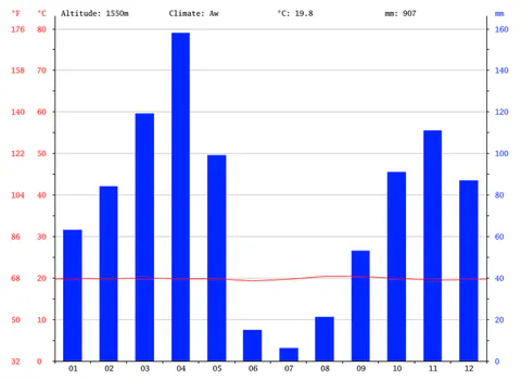
Eastern province, especially Gishari farm plantation type of rainfall, characterized by what is Known as moderate as heavy rains fall at the beginning at February to May and September to December of the year and lower rains fall towards the December mid to February mid and June to august end the year due to (Kim, 2018). There are eight rainfall measuring stations at Rwamagana plantation. Annual rainfall ranged from low of 850 mm in 2005 to high of 1200 mm in 2006. The study conducted by Juvenal and Eduard (2010) stated that in general Rwanda annual rain fall reduce gradually according to altitude.
A study conducted by Huang, Duiker, Deng, Fang, and Zeng (2015) stated that using 1960-2006 data in low, showed that high(low) yield are due to the part to sufficient rainfall in the second half of the growing season. The summers are much rainier than the winters in Rwamagana. This location is classified as Aw by Köppen and Geiger. In Rwamagana, the average annual temperature is 19.8 °C. The rain fall here averages 907 mm and altitude 1550m.
Minimum and maximum temperature
Temperatures required on carrots are a cool-weather crop that requires the right temperatures to produce a healthy crop production whereas warmer temperatures are only acceptable early in the growing process (Dukes, 2006; Salokhe, Babel, & Tantau, 2005). If you live in a coastal area with Mediterranean climates, you may start growing carrots in the fall for a winter harvest. Those in warmer inland areas should avoid planting carrots at warmer times of the year, as the carrots will grow slowly and produce little. The study conducted by Sebaziga Ndakize (2018) stated that Rwanda accounts some micro climates zone which has high deviation value from annual average temperature and yet temperature has significant impact on development and productivity crop. In addition, the research done by Rahman, Kang, Nagabhatla, and Macnee (2017) stated that monthly mean, maximum and minimum surface air temperature data were employed to study the variability.
According to Autovino, Rallo, and Provenzano (2018) Ordinary line regression (OLR) (y = αt + β) is an acknowledged way to capture correlation; where the rate of change is expressed as α and monthly and seasonal temperatures as y at the given time, t. The gradient of trends was calculated using the slope of the linear tendencies expressed in °C per decade.
The study conducted by Liyanage et al. (2016) stated that daily weather data of maximum temperature, minimum temperature, and relative humidity for 10 years were averaged on a weekly basis. The IDW interpolation technique was used to prepare thematic maps. According to the research conducted by Sammis and Wu (1985), it was revealed that temperature variation affected the crop yield under drip irrigation system. For instance, research work done by Liao, Zhang, and Bengtsson (2008) proved that the maximum temperature grouped as 27°C-32°C, 32°C-35°C, and more than 35°C affected water consumption of spring wheat and their effects on crop yield was high. In addition, their results showed that minimum temperature is not in the critical level for carrot cultivation within Kurunegala District throughout the year because its Maximum temperature is (150C - 200C) (El–Aref, Abdel–Mawly, & Abo–Elhamd, 2005).
According to the study conducted by Nsengiyumva, Luo, Nahayo, Huang, and Cai (2018) stated that the maximum day time temperatures usually occur between 3 pm and 7 pm, while the minimum temperatures usually occur between 4 am and 9 am. These times vary depending on sky condition, wind direction and speed as well as a host of other factors. Rwanda Meteorological Agency (2018) stated that the minimum temperatures usually occur during the hours immediately before or after sunrise. In the winter this can be as late as 9 am, while in the summer it can be as early as 4 am. As with winter time maximum temperatures a strong frontal system can move through a region during the day causing falling temperatures through the afternoon and evening results in the minimum occurring much later than normal (Mostovoy, King, Reddy, Kakani, & Filippova, 2006; Whiteman, Haiden, Pospichal, Eisenbach, & Steinacker, 2004).
The study conducted by Sridevi and Chellamuthu (2015) proved that rice is most sensitive to high temperatures at heading and next most sensitive at about 9 days before heading. One or two hours of high temperature at a thesis has a decisive effect on the incidence of sterility. Furthermore, Sridevi and Chellamuthu (2015) showed that High temperatures before or after anthesis have much less effect on sterility. The high sterility may be attributable to failure of fertilization caused by the imperfect splitting of anther or wilting of stigma induced by high temperature and low humidity. High temperature desiccated pollens (Sridevi & Chellamuthu, 2015). Sterility was increased at high temperature of 35 ºC (day) and 30ºC (night) as a result of smaller pollens and non-dehiscence of anthers. The study done by Shah et al. (2011) stated that the reduced yield was a result of poor pollen shedding as well as inadequate pollen growth in temperature above about 34 ºC. The day time temperature of 32º to 38 ºC caused sterility, depending on the cultivars.
Relative humidity
According to Coelho and Harnby (1978), Relative humidity is the ratio of the partial pressure of water vapour to the equilibrium vapour pressure of water at a given temperature. Relative humidity depends on temperature and the pressure of the system of interest. The same amount of water vapour results in higher relative humidity in cool air than warm air also it explain as channel describing a function of temperature and moisture in the atmosphere and establish amount of humidity in which occupied there. Relative humidity is invariably much more in the morning than in the afternoon. Carrot which is cultivated in the region of an environment with lower relative humidity (Bos, Kselik, Allen, & Molden, 2008).
Meteologist often use the relative humidity as a measurement explaining the weather at various place, whereas temperature is warm the increase water vapour in the air (atmosphere), indeed the coldness appear. The research conducted by Gosselin et al. (2016) stated that relative humidity was grouped into three classes as 60% - 80%, 80% - 85% and more than 85% (Gosselin et al., 2016). The temperature maps and relative humidity maps were overlaid with the weighted sum technique giving weights as 0.75 and 0.25 respectively to produce suitability maps for carrot cultivation on weekly basis throughout the year. Relative humidity in all three ASCs is more than 85% during Maha season and in between 80 % and 85 % during season. Humidity is the water content of the mixture of water vapor and other elements found in the air while relative humidity is the percentage of water vapor in the air at a given temperature (Gosselin et al., 2016).
The study conducted by Doerr, Dekker, Ritsema, Shakesby, and Bryant (2002) stated that parameters for expressing humidity and temperature are interconnected, so it is calculating in percentage is follow: RH=100ꓫAa/Es ,Where: A is saturated vapor pressure(specific humidity) in KPa calculated using equation Es=0.6108exp (17.2694T/(273+T), Es is obsolute humidity, where T is the temperature in 0C, then Ea was calculating using As and RH and is using to express the moisture profiles KPa (Doerr et al., 2002).
Wind velocity
The research conducted by Gao et al. (2014) reported that in case of estimating crop water requirement and wind speed should be always be calculated as height higher than 2m with equation below:
U2= Uh
U2 is the wind speed at 2m above the ground surface, ms-1
h is the height of the measurement above the surface, m
Uh is the measured speed at a certain height ‘h’ above the ground surface. The study conducted by Kono and Takahashi (1964) stated that the lodging of crops is usually caused by wind and for rain. As for the difference in the plant position when it receives the wind force; the magnitude of the bending moment varied by more than about 20 per cent. In addition, research done by C.-M. Yang, Fan, and Hsiang (1993) stated that the higher wind speed during the booting stage and mature stage of the second crop adversely affect plant height spikelet number and fertility rate consequently lower the yield (C.-M. Yang et al., 1993).
Sunshine hours
The research conducted by Safari and Gasore (2009) reported that eastern province is the driest province over all the country, begging by January shows the long day light duration that are ranging from 12:11:-12:12 in hours and minutes. The shortest daylight mostly occurs in April which is ranging from 6-8hours by day. The research conducted by Ekhmaj and Alwershefani (2017) stated that the sunshine duration is an essential atmospheric indicator which is used in many agriculture, architects and solar energy applications. Furthermore, the results of Y. Yang, Zhao, Hu, and Zhou (2009) stated that the decline in sunshine hours in the region is heavily influenced by wind speed. Low dispersion of air pollutants and their aerosol derivatives under low wind speed are likely the cause of the decline in sunshine hours (Y. Yang et al., 2009).
Intensity of sunshine hours
According to Augustine and Nnabuchi (2009), The Sun is considered to produces a constant amount of energy. At the surface of the Sun the intensity of the solar radiation is about 6.33×10⁷ W/m2 (note that this is a power, in watts, per unit area in meters) ,Solar radiation, energy from the sun, in the form of sunlight, supports life on Earth and drives the Earth's climate and weather. Solar radiation is the electromagnetic radiation emitted by the sun. The sunlight intensity and the related energy received is call the solar constant. Depending on the angle of the sun sunlight travels different path length described by the Air mass (Augustine & Nnabuchi, 2009; Muzathik et al., 2011).
Soil properties on carrot production
According to the research conducted by Ding et al. (2013), Sandy soils, sandy loam and silted loam are traditionally considered the best soils for carrots. Heavy, clay soils or compacted soils may produce a warped or stunted crops. Amend clayey soils should with loam builder or organic material to create a lighter, better-draining soil Carrots are a cool-weather crop that require the right temperatures to produce a healthy crop. Warmer temperatures are only acceptable early in the growing process. If you live in a coastal area with Mediterranean climates, even climate of Rwamagana in Gishari farm carrot grow because its soil characteristics as it mentioned above ,you may start growing carrots in the fall for a winter harvest. Those in warmer inland areas should avoid planting carrots at warmer times of the year, as the carrots will grow slowly and produce little (Rozek & Sady, 2000).
Soil physical properties
Bulk density (BD) on carrot production
The study conducted by Bennie and Hensley (2004) stated that soil bulk density is an indicator or measure of the compactness of specific soil. The study conducted by Hadebe and Van der Westhuizen (2005) states that tillage may also lead to the breakdown of organic matter, loss of soil moisture and an increase in wind and water erosion. Compaction may restrict soil aeration and crop root development, limiting water uptake, nutrient availability and overall crop growth. As far as the physical and chemical soil environment is concerned, the formation of organic soil matter provides feedback on the activity of decomposers and the plant community since it affects the retention of water and chemical properties, the germination of seeds and the distribution and activity of plant roots, while the regulation of turnover is the main feature of the decomposition subsystem (Lehmann et al., 2011). BD of soil samples has been measured using a cylindrical core cutter of 10 cm diameter and 13 cm length. The volume and weight of core cutter was determined. Core cutter was hammered down into the soil with rammer. The weight of soil with core cutter was determined again. It was calculated by:
Where, BD: bulk density (g/cm3); W₁: weight of core cutter (g); W₂: weight of core cutter and soil (g); V: volume of core cutter (cm3).
Soil texture and weight
According to Hamoud et al. (2019), the research findings proved irrigation regime and soil clay content had significant effects on growth, yield and water productivity of carrot. However, their combination showed no significant impact on panicles number, root biomass, harvest index and irrigation water productivity. Higher soil clay content results in increase in growth, yield, and water productivity of carrot.
Furthermore, the research conducted by Hamoud et al. (2019) stated that usually, paddy soil contains more clay, which is the most important component of mineral soil due to its very high specific surface area and consequently its ability to hold chemical properties and water. When the soil contains at least 35% of clay separate, it is designated as clay-textured soil where the characteristics of the clay separate are distinctly dominating. The formation of cracks in clay-textured soils is a natural phenomenon and physical manner with important agricultural repercussions. Soil desiccation is mainly governed by the properties that vary in space such as moisture content and clay content. Hamoud et al. (2019) stated that a great amount of clay in soil results in large specific surface area, thus results great shrink-swell potential of the soil. Hamoud, Guo, Wang, Chen, and Rasoul (2018) stated that studies displayed a positive and strong correlation between expansive soil potential and total clay content. Since water is the main governing factor for shrinking and swelling of soils and development of fractures, irrigation regime is as important as soil clay content on this aspect. Carrot grows well because soil swelling is widely recognized because the fine clay absorbs water.
The study conducted by Hamoud et al. (2018) stated that in Alternate Wetting and Drying (AWD), the soil is allowed to dry out to some certain degree before next round irrigation, at that time the top layer of the soil cracks due to the limiting of water from emitters within soil-clay microstructures. During the irrigation-dry out cycles, the increase in occurrence and extent of cracks results in significantly higher penetration rate. Banerjee, Yesmin, and Vessey (2006) stated that cracks influence root development and nutrient and Water absorbance, further influences the process of plant growth and development in soils. Also, desiccation cracks serve as secondary evaporation plates to increases the evaporation of water from cracked soils as per DeCarlo and Shokri (2014), further decreased water use efficiency as per Alam (2017).
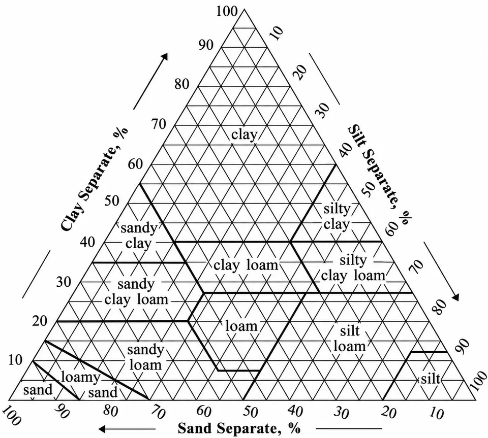
Virginia State University stated that they have developed a field test kit indicators of soil quality attributes. There are 12 soil textural classes represented on the soil texture triangle. This triangle is used so that terms like “clay” or “loam” always have the same meaning. Each texture corresponds to specific percentages of sand, silt, or clay. Knowing the texture helps to manage the soil. It also specified the texture triangle based on silt, sand and clay percentage of the soil. It also provides the texture of the soil based on bulk density of the soil (Weipeng et al., 2015). The relative size distribution of the mineral soil particles is called soil texture. There is no universal particle size classification. The most prevalent schemes are presented in figure 1. Particles between 2 mm and 7.5 mm are called gravel (2-4mm), pebbles(4-76mm),cobles(76-250mm) and still larger ones boulders greater than 600mm or stones (250-600mm). Each size class of soil particles is called a soil separate or textural fraction. A classification of soils based on only three size classes: sand, silt and clay is presented by the textural triangle in figure 2. The triangle applies for mineral soils and is based on the classification of the USDA. For a granulometric analysis the soil sample is dried, carefully grinded and separated into size groups by sieving through graded sieves, down to a diameter of 50 pm (Lal & Shukla, 2004).
| US Department of agriculture classification (USDA) | |||||||
|---|---|---|---|---|---|---|---|
| 0.002 | 0.05 | 0.1 | 0.25 | 0.5 | 1.0 | 2.0 mm | |
| Clay | Silt | Very fine | Fine | Medium | Coarse | Very coarse | Gravel |
| Sand | |||||||
| Clay | Silt | Sand | Gravel | ||||
| Fine | Coarse | ||||||
| 2 | 20 | 200 | 2000 μm | ||||
| International soil society classification (ISSS) | |||||||
Classification of still finer particles is generally obtained from the settling velocity of the particles after dispersion of the sample in water. The rate of sedimentation is according to Stroke’s law related to the particle diameter. Each soil separate is expressed in grammes per 100 g of gravel-free mineral matter. The result obtained with the so-called mechanical analysis is the laboratory texture; field texture is determined by finger texturing of moist soil in the field (coarse and gritty, or fine and smooth). The organic matter is usually specified as a separate fraction. In mineral soils hydrogen peroxide is used to remove the organic matter. In organic soils the organic matter is determined from the loss in weight of the oven-dry sample upon complete oxidation of the organic matter at about 9000c (Gough & Wolf, 1996).
Un-weathered fragments (stones, gravel) and weathered components of parent material such as quartz, feldspars and mica's constitute the sand and silt fractions and are called primary minerals. The primary minerals have a low specific surface, are relatively chemically inert and may supply chemical properties to the soil upon further weathering. Secondary minerals, such as oxides and hydroxides of Fe and AI, and in particular clay minerals are the products of complex chemical weathering. The clay fraction determines the properties of the soil most decisively because of its large specific surface and chemical activity (see figure 2.1). The study conducted by Hamoud et al. (2018) stated that irrigation regime is the main factor in determining water consumption and the efficiency of water use in carrot cultivated in the clay-textured soil. The increase in soil clay content from 40% to 60% increased growth, yield, and water productivity of carrot.
Porosity of soil on carrot production
According to Lipiec et al. (2003), soil Porosity is a measure of how much of a rock is open space. This space can be between grains or within cracks or cavities of the rock whereas Permeability is a measure of the ease with which a fluid (water in this case) can move through a porous rock, Soil porosity" refers to the amount of pores, or open space, between soil particles (Guéguen & Palciauskas, 1994). Pore spaces may be formed due to the movement of roots, worms, and insects; expanding gases trapped within these spaces by groundwater; and/or the dissolution of the soil parent material. Soil texture can also affect soil porosity (Lipiec et al., 2003).
Soil permeability
According to Quirk (1986) Soil permeability is the property of the soil to transmit water and air and is one of the most important qualities to consider for fish culture. The permeability of soil describes how water (or other liquid) and air are able to move through the soil. In the case of rainfall or irrigation, water moves very easily through highly permeable soils and very slowly through soils with low permeability (Cote, Bristow, Charlesworth, Cook, & Thorburn, 2003). The permeability of a soil can be determined by calculating its infiltration rate. Soils with sandy textures have large pore spaces that allow rainfall to drain very quickly through the soil. Sandy soils are known to have high permeability, which results in high infiltration rates and good drainage. Clay textured soils have small pore spaces that cause water to drain slowly through the soil. Clay soils are known to have low permeability, which results in low infiltration rates and poor drainage (Iversen, Moldrup, Schjønning, & Loll, 2001).
As more water fills the pore space, the air is pushed out. When all pore spaces in the soil are filled with water, the soil becomes saturated. The roots of many types of plants are not able to survive in saturated soils (Glinski, 2018). Saturated soil on level ground results in standing water which can cause flooding. Saturated soils on sloping ground results in runoff, and may lead to an increased volume of water entering a body of water. This condition can result in erosion and flooding, as well as an increased level of pollutants entering the body of water. The water table is the surface below ground where water-saturated soils meet air-saturated soils. How deep this zone is changes from season to season and from year to year because rainfall and vegetation change; in wetter years, the water table moves up closer to the surface. If you are putting in a well for your home, you are definitely interested in where the water table is. The deeper the water table, the more it costs to put in the well (Cote et al., 2003).
Comparison of soil texture and soil bulk density as per the USDA-NRCS guidelines
The Soil Quality Kit guidelines given by the USDA, Natural Resources Conservation Services were used to get the soil texture of the experimental plots based on bulk density of the soil. The USDA NRCS guidelines are given below in Table 2.
| Soil texture | USDA-NRCS guidelines Bulk Density (BD) in gm/cm3 and soil texture | ||
|---|---|---|---|
| Ideal BD for plant growth | BD that affect root growth | BD that restrict root growth | |
| Sands, loamy sands | < 16.0 | < 1.69 | > 1.80 |
| Sandy loams, loams | < 1.40 | < 1.63 | > 18.0 |
| Sandy clay loams, clay loams | < 1.40 | < 1.60 | > 1.75 |
| Silts, silt loams | < 1.30 | < 1.60 | > 1.75 |
| Silt loams, silty clay loams | < 4.40 | < 1.55 | > 1.65 |
| Sandy clays, silty clays, some clay loams (35 -45% Clay) | < 1.10 | < 1.49 | > 1.58 |
| Clays (> 45% clay) | C 1.10 | < 1.39 | > 1.47 |
Infiltration rate of the soil
According to Parr and Bertrand (1960), the infiltration rate is the velocity or speed at which water enters into the soil. It is usually measured by the depth (in mm) of the water layer that can enter the soil in one hour. An infiltration rate of 15 mm/hour means that a water layer of 15 mm on the soil surface will take one hour to infiltrate. According to Kirkham (2014), the Infiltration rate may be defined as the meters per unit time of water entering into the soil regardless of the types or values of forces or gradients. The term hydraulic conductivity, which has been defined as the meters per day of water seeping into the soil under the pull of gravity or under a unit hydraulic gradient, should not be confused with infiltration rate. Infiltration rate need not refer to saturated conditions. If two rain drops of total volume 2 mm3 = 0.000002 m3 fall per day on a m2 of soil and are absorbed into the soil, the infiltration rate is 0.000002 m/day. Water entry into soil is caused by matric and gravitational forces. Therefore, this entry may occur in the lateral and upward directions as well as the downward one. Infiltration normally refers to the downward movement. The matric force usually predominates over the gravitational force during the early stages of water entry into soil, so that observations made during the early stages of infiltration are valid when considering the absence of gravity (Parr & Bertrand, 1960).
If water infiltrates into a dry soil, a definite wetting front, also called a wet front, can be observed. This is the boundary between the wetted upper part of the soil and the dry lower part of the soil. If water is infiltrating into soil contained in a clear plastic column, one can observe the progress of the wet front and mark wet fronts as they change with time. At present, it is impossible to measure the matric potential exactly at the wet front, because it progresses too rapidly into the soil (Beven & Germann, 2013). However, one can measure the amount of water infiltrated and the depth and shape of the wet front, and come to important conclusions about the entry of water into the soil. Infiltration is extremely important, because it determines not only the amount of water that will enter a soil, but also the entrainment of the “passenger” chemicals (chemical properties, pollutants) dissolved in it (Fagbenro, 2016; Olorunfemi & Fasinmirin, 2012).
Hydraulic conductivity of the soil
According to Kasenow (2002), Hydraulic conductivity is the ease with which water moves through porous spaces and fractures in soil or rock. It is subject to a hydraulic gradient and affected by saturation level and permeability of the material (Kasenow, 2002). Hydraulic conductivity is generally determined either through one of two approaches. The soil’s hydraulic conductivity was defined as follow in Darcy’s Law. It showed that V=-k dh/dx where v = apparent velocity of the groundwater (m/d), K = hydraulic conductivity (m/d), h = hydraulic head (m), x = distance in the direction of groundwater flow (m) (Fagbenro, 2016).
Soil moisture content
According to Verstraeten, Veroustraete, and Feyen (2008), Soil moisture is defined as the quantity water stored in the soil and is affected by precipitation, temperature, soil characteristics, and more air and water, the gas and liquid phases exist in the pores. The size of the soil particles and pores affects how much water a soil can hold, and how that water moves through the soil.
Chemical properties of soil
Cation Exchange Capacity (cec)
According to Aprile and Lorandi (2012), the Cation-exchange capacity (CEC) is the maximum quantity of total cations that a soil is capable of holding, at a given pH value, available for exchange with the soil solution. CEC is used as a measure of fertility, nutrient retention capacity, and the capacity to protect groundwater from cation contamination. It is expressed as centi-mol of Hydrogen per kg (cmolc/kg or 100 meqc/100g). Most of the soil's CEC occurs on clay and humus. It the most cases, it is also expressed in parts per million (ppm) or meq/L or mg/L (Aprile & Lorandi, 2012)
Soil pH
According to Pietri and Brookes (2008), Soil reactivity is expressed in terms of pH and is a measure of the acidity or alkalinity of the soil. More precisely, it is a measure of hydrogen ion concentration in an aqueous solution and ranges in soils from 3.5 (very acid) to 9.5 (very alkaline). The effect of pH is to remove from the soil or to make available certain ions. Soils with high acidity (<5.5) tend to have toxic amounts of aluminium and manganese. Soils with high alkalinity (>8.5) tend to disperse. Soil organisms are hindered by high acidity, and most agricultural crops do best with mineral soils of pH 6.5 (Van Lierop, 1990).
Base saturation percentage
There are acid-forming cations (hydrogen and aluminium) and there are base-forming cations (calcium, magnesium, potassium and sodium). The fraction of the base-forming cations that occupy positions on the soil colloids is called the base saturation percentage. When the soil pH is 7 (neutral), base saturation is 100 percent and there are no hydrogen ions stored on the colloids. Base saturation is almost in direct proportion to pH and except for its use in calculating the amount of lime needed to neutralize an acid soil, it is of little use (Agbugba, 2018).
Plant chemical properties
According to Warner (1967), Sixteen chemical properties are essential for plant growth and living organisms in the soil. These fall in two different categories namely macro- and microchemical properties. The macrochemical properties include Carbon (C), Oxygen (O), Hydrogen (H), Nitrogen (N), Phosphorus (P), Potassium (K), Calcium (Ca), Magnesium (Mg), Sulhpur (S) and are the most essential chemical properties to plant development whereby a high quantity of these is needed. The microchemical properties on the other hand are needed in smaller amounts, however they are still crucial for plant development and growth, these include Iron (Fe), Zinc (Zn), Manganese (Mn), Boron (B), Copper (Cu), Molybdenum (Mo) and Chlorine (Cl). Nearly all plant chemical properties are taken up in ionic forms from the soil solution as cations or as anions (Bhattacharya, 2011).
Organic soil carbon
According to Lee et al. (2009), The carbon that is fixed by plants is transferred to the soil via dead plant matter including dead roots and leaves. This dead organic matter creates a substrate which soil micro-organisms respire back to the atmosphere as carbon dioxide or methane depending on the availability of oxygen in the soil. Soil organic carbon can also be oxidized by combustion and returned to the atmosphere as carbon dioxide. Some of the carbon compounds are easily digested and respired by the microbes resulting in a relatively short residence time. Others, like lignin, humic acid or substrate encapsulated in soil aggregates, are very difficult for the biomass to digest and have very long residence times. Soil organic carbon improves the physical properties of the soil. It increases the cation exchange capacity (CEC) and the water-holding capacity and it contributes to the structural stability of clay soils by helping to bind particles into aggregates. Soil organic matter, of which carbon is a major part, holds a great proportion of chemical properties, cations and trace elements that are of importance to plant growth. It prevents nutrient leaching and is integral to the organic acids that make minerals available to plants. It also buffers soil from strong changes in pH. It is widely accepted that the organic carbon content of the soil is a major factor in its overall health, is a major part of the Carbon Cycle and an important factor in the mitigation of climate change effects (Lee et al., 2009).
Soil nitrogen
According to Metcalfe (2008)Nitrogen is the most critical element obtained by plants from the soil and when deficient is a bottleneck in plant growth. Plants can use the nitrogen as either the cation ammonium, NH4+, or the anion nitrate, NO3-. Nitrogen is seldom missing in the soil, but is often in the form of raw organic material which cannot be used directly. Nitrogen is also available in gas forms in the soil, however these quantities are very small and difficult to detect such as: nitrous oxide (N2O), nitric oxide (NO), nitrogen dioxide (NO2), ammonia (NH3) and molecular nitrogen (N2) present in the air space of the soil (Metcalfe, 2008).
Soil salinity or Electrical conductivity
According to Christen and Ayars (2001), Salts can be transported to the soil surface by capillary transport from a salt laden water table and then accumulate due to evaporation. Salinization occurs when irrigation practices are carried out without due attention to drainage and leaching of the salts out of the soil. Salts can also accumulate due to seawater intrusion, or may occur naturally. As soil salinity increases, salt effects can result in degradation of soils and vegetation. The most common salts are combinations of the cations sodium, calcium, magnesium and potassium with the anions chlorine, sulfate and carbonates (Christen & Ayars, 2001).
Soil sodicity/ Soil alkalinity (SAR)
According to Rengasamy and Olsson (1991), Sodicity refers to an excess of exchangeable sodium in the soil. Sodic soils tend to occur general within arid to semiarid regions and are often unstable, exhibiting poor physical and chemical properties, which impede water infiltration, water availability, and ultimately plant growth (Rengasamy & Olsson, 1991).
Calcium carbonate content
According to Horneck, Ellsworth, Hopkins, Sullivan, and Stevens (2007), Calcium carbonate CaCO3, is a salt that is not very soluble and occurs in various forms and concentration in soils. Calcium carbonate in moderate amounts is favourable for soil structure and is often used to correct the pH of acidic soils, but when the level of calcium in the soil exceeds the capacity of the soil to absorb it, it binds with other elements and forms insoluble compounds that are difficult for plants to absorb. Excess amounts of calcium may restrict the availability of phosphorous, boron and iron to plants (Horneck et al., 2007).
Calcium Sulfate (Gypsum) content
In soils substantial secondary accumulation of gypsum (CaSO4.2H2O) may occur, particularly in the driest climates. The soils affected by gypsum are developed in mostly unconsolidated alluvial, colluvial and aeolian deposits of base-rich weathering material. The natural vegetation on soils with high gypsum content is sparse and dominated by xerophytic shrubs and trees and/or ephemeral grasses (Deckers & Nachtergaele, 1998).
Crop Water Requirement of Carrot
According to Qadir and Oster (2004), Water management efficiency is a key issue for sustainable agriculture development, since it is necessary to get a higher biomass production per unit of applied water. This study aimed to determine both water requirements and water use efficiency (WUE) and their effect on yield and quality parameters in carrots (Daucus carota L.) (Qadir & Oster, 2004).
Use of crop water 8.0 software
According to Rose, Sankaranarayanan, Pande, and Das (2019), the CROPWAT software 8.0 demonstrated by FAO was used to find out the crop water requirements, irrigation requirements of carrot and irrigation schedule. CROPWAT program helps farmers as per Rose et al. (2019) to assess the level of risk in their farm, based on crops they cultivate and hence agricultural advisory service people should be coached on software of CROPWAT 8.0 program, therefore, they will be considered helpful to farmers. CROPWAT was used to estimate the yield reduction caused by water stress and climatic impacts, which makes this model as a best tool for irrigation planning and management in maize as per (Kato & Tu, 2020).
Input weather data fed into CROPWAT (weather, soil and crop)
The program used for simulating crop yield response to water (CROPWAT) is a decision support system developed by the Land and Water Development Division of the FAO (AQUASTAT, 2009). Its main functions are to calculate reference evapotranspiration, crop water requirements and crop irrigation requirements in order to develop irrigation schedules under various management conditions and scheme water supply and to evaluate rain fed production, drought effects and efficiency of irrigation practices. It uses procedures for predicting yields when all the climate, soil and crop parameters are known. This approach allows estimation of ETa and Ks, from the ratio of actual to potential yield (AQUASTAT, 2009).
Getting outputs from cropwat
According to Rose et al. (2019) stated that CROPWAT is a FAO model for irrigation management which integrates data on climate, crop and soil to assess reference evapotranspiration (ETo), crop evapotranspiration (ETc) and irrigation water requirements develop irrigation schedules under various management conditions and scheme water supply. Proper and optimal scheduling of irrigation using CROPWAT 8.0 enabled the efficient water use to 70%. In addition, Ali et al. (2017) stated that the higher irrigation requirements during drier months of a season are explained by the severe drought condition and low relative humidity due to lack of rain and high temperatures, which led to increase evapotranspiration. Also observed that when the hottest period with the highest temperature prevailed, high evaporation occurred with rapid decrease in soil moisture implying the highest agricultural water requirement (Rose et al., 2019).
Reference Evapotranspiration (ETo)
Rose et al. (2019) Stated that the CROPWAT was used to estimate the annual reference evapotranspiration of 1967 mm in Northern Benin)] and the lowest monthly value of annual reference evapotranspiration was found to be 123 in August month. The crop evapotranspiration and the crop irrigation requirements were estimated at 651mm and 383mm respectively in rainy season and 920mm and 1148mm in dry season respectively. Rose et al. (2019) stated that the model estimated mean annual reference evapotranspiration of rice crop, which was 1408 mm for western part of Bangladesh. The observed ETo values were higher during March to August and lower during September to February .The highest monthly ETo(175 mm) was found in April and the lowest (70 mm) in December (Rose et al., 2019).
Effective Rainfall
According to Surendran, Sushanth, Mammen, and Joseph (2017) stated that the CROPWAT was used to find out the crop water requirements of crops in agro-ecological units of Palakkad district of humid tropical Kerala). The major cultivated crops are rice, coconut, banana, are can vegetables, pulses, rubber, tea, coffee, cotton etc. The total water requirement for these crops in various agro-ecological zones has been computed. Using the evapotranspiration (ETO) and effective rainfall in each agro-ecological unit, a climatic water balance has been worked out. Surendran et al. (2017) stated that the rain data was also collected from the Agro meteorological station and applied in CROPWAT software to obtain effective rainfall (Surendran et al., 2017).
Net Irrigation Requirement (NIR)
According to Shah et al. (2015) stated that the CROPWAT was used to find out the crop water requirements for sorghum, which was 187.5 mm). The net irrigation requirements for sorghum at fixed interval per stage is 173.3 mm and four irrigation are on date 3-Sep, 28-Sep, 17-Nov, 17-Dec with varying depth of 9.6 mm, 3.9 mm, 111.4 mm, 48.4 mm respectively. In addition, Rose et al. (2019) reported that the Sugarcane crop in the developing stage it requires Net irrigation of 196.7 mm, Gross irrigation of 281.0 mm and flow of 0.66 L/s/ha. And at the 109th day of mid stage it requires Net irrigation of 196.8mm, Gross irrigation 281.1mm and Flow of 0.54 L/s/ha and at the 155th day of the mid stage it requires Net irrigation of 199.4mm, Gross irrigation of 284.9mm and Flow of 0.72 L/s/ha (Rose et al., 2019).
Irrigation Scheduling
Moisture management throughout the growing season is a critical factor for production of high quality crops. Even relatively short periods of inadequate soil moisture can adversely impact on many crops. Central to that management is appropriate irrigation scheduling (Fereres, Goldhamer, & Parsons, 2003). Irrigation scheduling is a management practice used to determine how often to irrigate, how much to apply and where to apply the water with each irrigation. Proper scheduling is essential for efficient use of water, energy and other production inputs such as fertilizer. It allows irrigations to be coordinated with other activities including cultivation and chemical applications (Waraich, Ahmad, Ashraf, Saifullah, & Ahmad, 2011). Efficient irrigation can be described as applying the crop’s water needs as required to sustain optimum growth and production at the lowest capital and operating costs possible. Efficient irrigation is obtained by correctly designing and operating the irrigation system to match, crop and soil management limitations (Oweis, Hachum, & Kijne, 1999).
To schedule your irrigation with confidence you need to understand how much water your soil can hold that is available to the crop. The soil surrounding plant’s roots stores the water it needs to live, grow and produce a crop. This water is held by the soil with increasing strength as the soil dries out (Garcia et al., 2018). Sandy soils are well known for their inability to hold water. Precise irrigation scheduling is required in these soil types to avoid unnecessary loss of water and chemical properties while providing a sufficient amount of water for optimum plant growth and production. In sandy soils very little water is stored in the root zone, and excessive water applications result in the loss of mobile chemical properties such as nitrogen due to deep percolation (Smajstrla, Haman, & Zazueta, 2005).There are two basic approaches to scheduling drip irrigation. These are soil based scheduling and evapotranspiration data based approach (DJ, 2005).
Evapotranspiration data can be used to schedule trickle irrigation systems using a plant water requirement or water budget method. The plant water requirement method adjusts the trickle system operating time by comparing the actual ET data to the theoretical Peak ET used in the design. This method can be used in situations where the system is designed to irrigate each individual plant with one or more emitters. The water budget method can be used for row crops such as vegetables, strawberries or any crop that is spaced close enough together so that the system is irrigating the entire field (Jones, 2004).Using a water budget to schedule trickle irrigation systems is similar to balancing a cheque book. The plant’s water storage reservoir can be considered as a bank. This reservoir can hold a limited amount of water that is useful for the Crop. Daily evapotranspiration amounts are reserved from the storage in the soil profile (Jones, 2004).
Chapter 3
Materials and methods
Introduction
This chapter deals with the materials used to achieve the expected results from different specific objectives. It also covers the description of the study area, materials used to carry out the research, methods adopted including descriptive analysis. It included also the use of CROPWAT8 version computer software to compute irrigation water requirement. Least Significance Difference (LSD) was used to test the significant experimental plot with higher carrot yield.
Location of study area
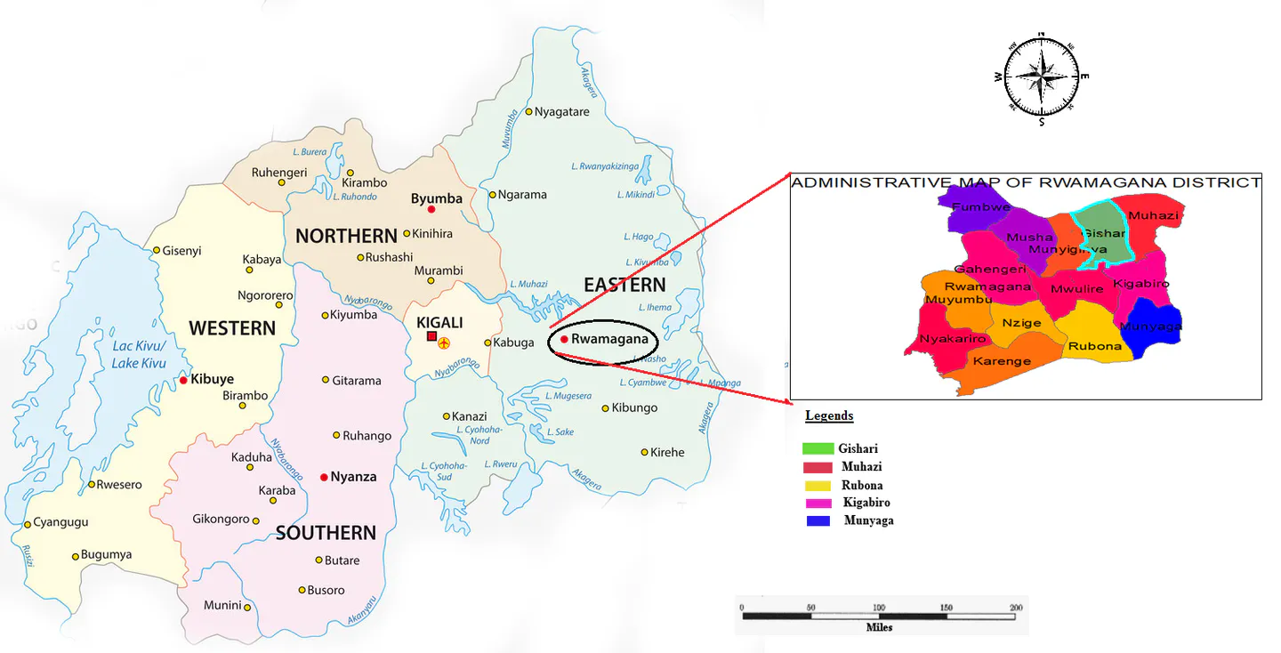
The study was conducted at IPRC Gishari farm which is located in Rwamagana District, Gishari sector. The geographical coordinates are of 1°57'12.65"S and a longitude of 30°26'19.12"E or -1.953513 and 30.438644 respectively. The topography characteristic slope land varies from 7-15% and precipitation less than 1500mm per year even altitude varies from 1480-1550m above sea level. The soils on the experimental site are Gishari farm soils which form the backbone of agriculture in Eastern in Rwanda. Map of Gishari sector is shown in Figure 2 using Arc GIS 10.4.
Materials used
The various materials used to carry out different specific objectives of the study are given in Table 3. The physical and chemical properties of the soil were carried out in the Huye soil Laboratory and the following list of materials was used.
Table 3: List of materials needed in the research
| S.No | Materials used |
|---|---|
| 1 | Hoe, Auger and shovel to take soil sample |
| 2 | Electronic balance |
| 3 | A.A.S Machine |
| 4 | PH meter (PH Probe ) |
| 5 | EC meter(EC Probe) |
| 6 | Nitric acid for titration process |
| 7 | Refrigerators to cool down the heated soil samples |
| 8 | Measuring tape meters to measure the dimensions of plots |
| 9 | Water tank of 10000 m3 |
| 10 | Pyrex beaker |
| 11 | Graduated cylinders for water volume measurement |
| 12 | Graduated pipettes |
| 13 | Chemical reagents |
| 14 | Laptop and software |
| 15 | CROPWAT 8 software |
| 16 | Soil shaker machine |
Methodology adopted
Different methods were adopted to reach the specific objectives like weather parameters on crop production, soil properties (Physical and chemical properties), water requirement and irrigation scheduling, uniformity coefficient and application uniformity of water and thereafter come up with estimation of yield of carrot under drip irrigation.
Analysis weather parameters on crop production
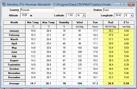
The weather data needed to analyse the performance evaluation of drip irrigation system on carrot production were rainfall, wind speed, maximum and minimum temperature, relative humidity and sunshine duration respectively. The collected data were sorted from 1989 up to 2019, it means that data for 30 years collected from Rwanda Meteorological Agency, in the sub -station of Kazo.
Determination of physical and chemical properties of soil
Soil sampling procedures and its collection
The following procedures were used for collecting the soil samples. The area to be sampled was cleared of any surface debris (e.g., twigs, rocks, litter). An area of approximately 10 cm in radius was created around the sampling location. Gradually, the auger was inserted into the soil by applying a downward force while rotating it. Once filled at the correct depth, the auger was removed and the top soil placed into a clean, dry container marked top soil. Augering was carefully done to prevent accidental brushing of loose material back down the borehole when removing the auger.
Core soil samples were taken from 10 plots selected from the IPRC Gishari farm under operational drip irrigation. The soil samples were taken 3 times in one place, mixed completely and look for the average mean soil sample of 200gm to used and then put the soil samples in a container. Repeat the process for all experimental soil plots (4plots) three times. The researcher repeated the process of soil sampling for all the four selected locations and there was the total number of 12 soil samples.
Soil bulk density
Core soil samples were taken from 4 soil plots of the selected farm of the experimental field with 1 soil sample per each plot. The representative soil sample was taken for laboratory analysis. The weight of the representative soil sample taken to laboratory was measured using an electronic balance in gm. The volume of the representative sample was measured by keeping it in a cylindrical box. The volume of soil was calculated by multiplying the bottom area of the cylindrical box and the height of the soil in the box.
Bulk density of soil = gm/cm3
Soil Porosity
Soil porosity is the volume of soil not occupied by solids and can be filled with air or water. Volume of soil pores and concentration of organic matter are greatest nearest the soil surface and decline with depth. According to density of water 1 gm of water is equal to 1 cm3 volume of water. Hence, the volume of air space in the soil is the weight of water added expressed in cm3. It is the volume of void. The soil porosity is measured using the formula given below.
Soil Porosity = x 100
Soil texture
Core soil samples were taken from 10 soil plots of the experimental field with 1 soil sample per each plot. The representative soil sample was taken for laboratory analysis. Sieve analysis consists of shaking the soil sample through a set of sieves that have progressively smaller openings. Soil texture analysis is the measurement of the proportions of the various sizes of the soil particles. The three major groups of soil particles are sand, silt and clay. The size measured for the particles change depending upon which system is used for defining soil particle size classification. Soil particles more than 2 mm were classified as coarse material. It can be removed first. Then the soil will be sieved to get sand, silt and clay with the following sizes.
Table 4: Classification of Soil texture based on size of particles
| Type of particles | Size of particles |
|---|---|
| Coarse material | Greater than 2 mm |
| Sand | - 0.05 mm |
| Silt | – 0.002 mm |
| Clay | Less than 0.002 mm |
The USDA texture triangle is used to classify the soil into twelve major soil texture classifications like sand, loamy sand, sandy loam, loam, silt loam, silt, sandy clay loam, clay loam, silty clay loam, sandy clay, silty clay, and clay. The USDA texture triangle chart was used to find out the soil texture of the experimental field based on the percentage of sand, silt and clay estimated in the laboratory using sieve analysis. Sieve analysis consisted of a sieve box with two sieves kept on a Roto machine for shaking. 100 gm of soil sample is taken and kept on the top sieve. The unit is shake for 5 minutes. Sand is retained on the top sieve, silt is retained on the bottom sieve and the fine clay particles are collected in the pan. The weights of retained materials were contented into percentage of sand, silt and clay. Using the percentage of sand, silt and clay, the soil texture can be found out from the USDA texture triangle.
Figure 3 shows the soil texture triangle
Comparison of soil texture and bulk density based on USDA-NRCS guidelines
The Soil Quality Kit guidelines given by the USDA, Natural Resources Conservation Services were used to get the soil texture of the experimental plots based on bulk density of the soil. The USDA NRCS guidelines are given below.
| Soil texture | USDA-NRCS guidelines Bulk Density (BD) in gm/cm3 and soil texture | ||
|---|---|---|---|
| Ideal BD for plant growth | BD that affect root growth | BD that restrict root growth | |
| Sands, loamy sands | < 16.0 | < 1.69 | > 1.80 |
| Sandy loams, loams | < 1.40 | < 1.63 | > 18.0 |
| Sandy clay loams, clay loams | < 1.40 | < 1.60 | > 1.75 |
| Silts, silt loams | < 1.30 | < 1.60 | > 1.75 |
| Silt loams, silty clay loams | < 4.40 | < 1.55 | > 1.65 |
| Sandy clays, silty clays, some clay loams (35 -45% Clay) | < 1.10 | < 1.49 | > 1.58 |
| Clays (> 45% clay) | C 1.10 | < 1.39 | > 1.47 |
Soil pH
Soil pH was determined by calibrating the pH reader (Hanna Instrumental pH Meter, model Hi 9032), using two buffer solutions, one buffer with neutral pH (7.0) and the other pH (4.0). The electrodes were then inserted into the beakers containing the two solutions alternatively, and the pH adjusted as required. Twenty-five (25) grams of the soil sample were weighed into a 100 ml beaker, and 25 ml of distilled water was added as a suspension medium. Samples were then stirred intermittently for 30 minutes using a glass rod. Using the calibrated pH meter, the pH readings were recorded.
Soil Electrical conductivity (EC)
Electrical conductivity was determined by electrical conductivity meter (Hanna Instrumental Conductivity Meter, model Hi 9032) in 1:5 soil water ratio (Jackson 1973). Forty (40) grams of the soil sample were weighed and placed into a 200 ml flask and 80ml of distilled water added. The conductivity electrodes were then washed with distilled water and rinsed with standard KCL solution. The conductivity meter was adjusted to read 1.412 mS/cm, corrected to 250C. The electrodes were then washed and dipped into the soil extract and the digital displays were recorded as the salt content in the extract, and an indication of salinity status of the soil sample. EC is typically reported in milliSiemans per centimetre (mS/cm) or microSiemans per centimetre (µS/cm).
Determination of calcium
For the determination of calcium, a 10 ml portion of the extract was transferred into an Erlenmeyer flask. To this, 10ml of potassium hydroxide solution was added followed by 1ml of triethanolamine. Few drops of potassium cyanide solution and few crystals of cal-red indicator were then added. The mixture was titrated with 0.02 N Ethylene diamine tetraacetic acid (EDTA) solutions from a red to a blue end point.
Determination of available potassium
Potassium present in the soil was extracted with neutral ammonium acetate of 1 molarity. This is considered as plant-available K in the soil. It was estimated with the help of a flame photometer (Toth & Prince, 1949). A standard curve was prepared by atomizing the flame photometer to 0 and 20 μg K per ml solutions alternatively to readings of 0 and 100. These readings were then plotted against the K contents and the points connected with a straight line to obtain a standard curve. Then 5 g of the soil sample were mixed with 25 ml of the ammonium acetate extractant into a conical flask
Soil Organic Matter Content (SOM)
Calcination method was used to determine the soil organic matter as discussed by (Sato et al., 2014). Following the laboratory procedures developed by (X. Wang, Smethurst, & Herbert, 1996) (Q. Wang, Li, & Wang, 2011), the researcher first place 10grs (W1) of soil samples taken in a from the field and heated at 105ºC for 3 hours to remove completely soil moisture using an oven dryer. After the researcher measured the weight of dried soil which is recorded (W2). The difference between W1-W2 is named moisture content based on weight basis. We then measured the weight of crucibles plus weight of dried soil to prepare the soils samples to be combusted in a programmable muffle furnace (S1849, KOYO LINDBEERE LTD) at 450ºC for Loss-on-ignition (LOI) Procedure for SOM for at least 8hours of operation. Then the new weight (W3) is recorded. Soil organic matter is calculated as the weight loss between 105ºC and 450ºC based on LOI (Lost on Ignition), then the remaining quantity is ash to be titrated in AAS machine for mineralization process.
The conversion constant of 0.273 in equation (3.11) is applied to convert mass of CO2 to mass of carbon.
Determination of Phosphorus
A standard curve was prepared by dissolving 0.3 g of pure dry KH2PO4 in 1litre of distilled water. Ten milliliters (10 ml) were taken from the solution and diluted to 0.5 millitres with distilled water. 1 ml of dilute SnCl2 solution was added, shaken and diluted to 25 ml mark. After 10 minutes, the blue colour was read from the spectrophotometer machine at a wavelength of 660 nm. The absorbance readings were then plotted against “µg P” and the points were connected. After the preparation of the calibration curve, 5 g of the soil sample was weighed and 50 ml of Bray‘s extractant No.1 were added into a 100 ml conical flask. The sample was shaken for 5 minutes and filtered. From the filtrate, 5 ml were taken with a bulb pipette into a 100ml flash and 5ml of the Molybdate reagent were added with another 1 ml of SnCl2. After 10 minutes, the blue colour was read from the spectrophotometer (Plate 4) at 660 nm after setting the instrument to zero with the blank prepared similarly but without the soil.
Total Nitrogen (TN)
Total nitrogen was determined using Kjeldahl method (Simonne, 1994). Kjeldahl method involves three steps: mineralisation, distillation and titration. Mineralization aims at changing the solution into minerals. We poured mineral organic matter and sulphuric acid with catalyst to the soil sample. The solution heated for 2 hours on a 300°c oven until the green colour appeared. Distillation aims at getting vapour condensation. After preparing of the distillation flask, 10 ml of sodium hydroxide and 10 ml of sulphuric acid were added into the mineralized solution. By evaporation, the nitrate solution collected in 5 ml of boric acid. Titration aims at getting the amount of Nitrogen. The distillate solution contained excess acid was titrated by sodium hydroxide until pink colour appeared as endpoint. The colour changed from green to pink then yellow. Then, the used volume of sodium hydroxide to nearest 0.01 ml of concentration was recorded.
Sodium Adsorption ratio (SAR)
Sodium adsorption ratio is a measure of the amount of sodium (Na) relative to calcium (Ca) and magnesium (Mg) in the water extract from saturated soil paste. It is the ratio of the Na concentration divided by the square root of one-half of the Ca + Mg concentration. The Sodium adsorption ratio (SAR) is an irrigation water quality parameter used in the management of sodium-affected soils. SAR allows assessment of the state of flocculation or of dispersion of clay aggregates in a soil. For Sodium Adsorption Ratio (SAR), it should be computed based on formula in the form of the ionic concentrations are expressed in meq/l.
Where SAR = Sodium Adsorption Ratio, = Sodium concentration, Calcium concentration, and = Magnesium concentration
Determination of crop water requirement and irrigation scheduling of carrot
Crop water requirements (CWR)
The crop water requirement (CWR) is the amount of water equal to what is lost from a cropped field by the ET and is expressed by the rate of ET in mm/day. Estimation of CWR is derived from crop evapotranspiration (ETc). The water requirement of crops is the amount of water that is required to meet the evapotranspiration rate so that crops may thrive. The evapotranspiration rate is the amount of water that is lost to the atmosphere through the leaves of the plant, as well as the soil surface. Therefore, in order to estimate the water requirement of a crop we first need to measure the evapotranspiration rate. The reference rate, ET0, is the estimate of the amount of water that is used by a well-watered grass surface that is roughly 8 to 15 centimeters in height. Once ET0 is known, the water requirement of the crop can be calculated. The evapotranspiration of a crop under irrigation (ETc in mm) is obtained by multiplying the reference evapotranspiration (ETo) with a crop and growing stage specific coefficient (ETc = Kc x ETo). This coefficient has been derived for four different growing stages: the initial phase (just after sowing), the development phase, the mid-phase and the late phase (when the crop is ripening to be harvested) (FAO, 1998). In general, these coefficients are low during the initial phase, after which they increase during the development phase to high values in the mid-phase and again lower in the late phase. In this study, the Kc is the crop coefficient which is the ratio of the crop ETc o the ET0 (Kc=ETc/ETo), and it represents an integration of the effects of four essential qualities that differentiate the crop from reference grass, and it covers albedo (reflectance) of the crop soil surface, crop height, canopy resistance, and evaporation from the soil.
Irrigation Water Requirement (IR)
The CROPWAT 8 version computer package could help to compute the daily water balance of the root zone as far as root zone depletion at the day’s end by the following equation.
Where Dr, i is the root zone depletion at the day’s end i(mm), Dr,i−1 is the water content in the root zone at the previous day’s end (mm), Pi is the precipitation on day i (mm), ROi is the surface soil run off on day i (mm), Ii is the net irrigation depth on day i which infiltrates the soil (mm), Cri is the capillary rise from the groundwater table on day i (mm), ETci is the crop evapotranspiration on day i (mm),and Dpi is the lost water of the root zone on day i (mm).
Irrigation scheduling
Irrigation Schedule determines the correct measure of water to irrigate and the correct time for watering. The CROPWAT 8 version computer package model calculates the ET0, CWR, and IRs to develop the irrigation schedules under different administration conditions and water supply plans. The purpose of irrigation scheduling is to determine the exact amount of water to apply to the field and the exact timing for application. The amount of water applied is determined by using a criterion to determine irrigation need and a strategy to prescribe how much water to apply in any situation. Hence the importance of irrigation scheduling is that it enables the irrigator to apply the exact amount of water to achieve the goal. This increases irrigation efficiency. Irrigation scheduling is the process of determining when to irrigate and how much water to apply per irrigation. Proper scheduling is essential for the efficient use of water, energy and other production inputs, such as fertilizer. It allows irrigations to be coordinated with other farming activities including cultivation and chemical applications.
Determination coefficient of uniformity and application uniformity of water
The evaluations of water application uniformity in this study were calculated with 2 methods. First, the uniformity of water applied from the drip irrigation system using discharge measurement data from emitters and the following equations were used to evaluate the drip system. The following equations were by (Karmeli & Keller, 1974) cited by (Clemmens & Molden, 2007) and employed to compute uniformity Parameters of the drip system. These two equations are simple and straight forward and are still widely used and written as:
1. Coefficient of Uniformity (CU):
2. Emission Uniformity (EU):
where: qi is the discharge of emitter i, q is the overall average of emitter discharges, n is the number of emitters, qlq is the average low-quarter emitter discharge, S is the standard deviation, CVM is the manufacturers’ coefficient of variation for emitters. The coefficient of variation (C.V.) is found according to the equation:
According to (Pizarro Cabello, 1996)the drippers should be classified into categories of quality in which C.V. is used. By the standards of ASAE EP 405.1 (2003), the emitters are classified according to the C.V. as: Excellent (<5%), Medium (5-7%); Marginal (7-11%), Poor (11-15%) and Unacceptable (>15%). For the practice of fertigation, dripping is more usual by applying water in the vicinity of the plants roots, increasing the capacity of chemical properties absorption. According to Borssoi, Vilas Boas, Reisdörfer, Hernández, and Follador (2012), this feature minimizes fluctuations in soil water potential allowing crops, such as radish, to develop under optimum conditions of productivity and quality.
Emission uniformity is expressed as a percentage, and is a relative index of the variability between emitters in an irrigation block. Emission uniformity is defined as the average discharge of 25% of the sampled emitters with the least discharge, divided by the average discharge of all sampled emitters from the experimental site. To identify the 25% (Lower quartile) sampled emitters with the least discharge rate, the discharge rate of all sampled emitters should be ranked from lowest to highest. Then 25% (lower quartile) of the emitters with the lowest discharge rate should be averaged together.
Keller and Karmeli (1975) proposed the ‘Emission Uniformity’ as the measure for the performance evaluation of the drip irrigation system. They proposed two measures viz. emission uniformity and absolute emission uniformity. These measures are now widely accepted to measure the performance of irrigation system when laid in the field. According to the author, the emission uniformity, EU, which is expressed as percentage is the ratio of the average emitter discharge from the lowest one fourth of the field data (obtained from arranging the emitter discharges in descending order) to the average discharge of all the data. EU is computed by:
Where, EU is the Emission Uniformity or DU distribution Uniformity coefficient expressed in percentage, qn = average of the lowest one fourth of the field data emitter discharges (Lh-1), and qa = average of all the field data emitted discharges (Lh-1) respectively. According to standards of ASAE EP 458 (ASAE, 2001), the emitters may be classified as far as the Emission Uniformity or DU distribution Uniformity coefficient are as follow: Excellent (> 90%); Good (75-90%); Regular (62-75%); Bad (50-62%) and Unacceptable (<50%). For having small dimensions, the irrigation by drippers show variations in flow due to construction failure. These variations present a normal distribution, allowing the use of statistical concepts for obtaining quantitative conclusions.
Data analysis and processing
All collected data including Weather data, soil physical and chemical properties were filed in Ms excel for descriptive statistics analysis. It was intended to determine the average mean, max and min, standard deviation and coefficient of variation from the data. Then the researcher used the SPSS 22.0 and STATA 13.0 to test the Least Significance Difference (LSD) from the 4 plots. The study also adopted the Analysis of Variance (ANOVA) to indicate the variation of parameters with sampled blocks. Weather data were analyzed also by using the CROPWAT 8.0 version computer package to compute the Crop water requirement, Irrigation requirement and net irrigation for carrot.
Chapter 4
Results and discussions
The analyses of different data collected as prescribed per chapter 3 were discussed here. This chapter brings out the suitable results and interpretations for better understanding. This chapter deals with study of assessing the performance evaluation of drip irrigation system on carrot production at IPRC Gishari Farm in Rwanda. The results and discussions are explained in the following order:
To study the weather parameters of the experimental site
The weather data were collected from Rwanda Metrological Agency for the period of 30 years since 1989 up to 2019. The studied weather parameters for carrot production under drip irrigation system were precipitation, Minimum and Maximum temperature, Relative humidity, wind speed and sun shine duration. The results from CROPWAT 8.0 computer package were presented and discussed in the following sub headings.
The study of Rainfall at iprc Gishari farm experimental site
The weather data collected about the precipitation for 30 years was converted in monthly data and then analyzed for easily interpretation. The mean monthly rainfall in mm were plotted in a graph for the twelve months and is presented in Figure 4 below.
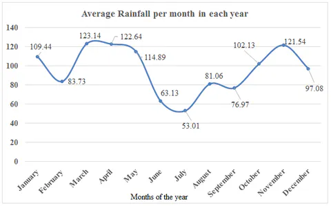
Based on results plotted on Figure 4, it was found that the highest rainfall was received during the month of March with average precipitation of 123.14mm followed by 122.64 mm during April. The lowest rainfall was recorded in the month of July with average rainfall of 53.01 mm and it is followed by the second lowest rainfall of 63.13 mm recorded in June. The difference between the highest and the lowest rainfall was found to be 70.13 mm. The driest months are June and July. It was found that the high rainfall periods are from January to May and from September to December. The twelve monthly rainfall was calculated and found to be 95.73mm/day. The monthly average rainfall from January to May was found to be 110.7 mm while the average monthly rainfall from September to December was found to be 99.43 mm respectively.
The study of Minimum and Maximum temperature at experimental site
The weather data collected about the minimum and maximum temperature for 30 years was converted in monthly data and then analyzed for easily interpretation. The average mean of monthly minimum and maximum temperature in ºC were plotted in a graph for the twelve months and is presented in figure 5 below.
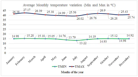
Based on results plotted on Figure 5, it was revealed that the average minimum temperature fluctuates between 15.28 ºC to 13.22 ºC recorded in the months of February and July respectively. The variation between the highest and the lowest minimum temperature is only 2.06ºC. The twelve monthly minimum temperature was calculated and found to be 14.7ºC. It implies that practically there is only two degree difference of minimum temperature variation during the twelve months. It was also found that the maximum temperature variation was ranging between 24.99ºC as the lowest and 26.9ºC as the highest average maximum recorded in May and September. The twelve monthly maximum temperature was calculated and found to be 26.8ºC The variation between the highest and the lowest maximum temperature is only 1.91ºC respectively.
The study of Relative humidity at the experimental site
The weather data collected from Rwanda Metrological station agency about the relative humidity for 30 years was analyzed. The results of the average mean monthly relative humidity expressed in percentage were plotted in a graph for the twelve months and is presented in figure 6.
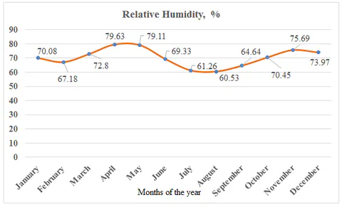
Based on the results plotted on Figure 6 shown above, it was found that the percentage of relative humidity was in range of 79.63% and 60.53% recorded in months of April and August. It was also found that the high relative humidity was recorded from January to June with relative humidity of 67.18% to 79.6% was found for the between January and June followed by the period of October to December with the relative humidity of 70.45% and 75.69% recorded in October and November. The twelve monthly relative humidity was calculated and found to be 70.39%. These have an implication that during these period there were the high rainfall associated with high relative humidity. It was also shown that the difference between the highest and lowest relative humidity was about 19.07% respectively.
The study of Wind speed at the experimental site
The weather data collected from Rwanda Metrological station agency about the wind speed for 30 years was analyzed. The mean monthly wind speed for daily data was recorded originally in m/s then converted into km/hour. The results of the average mean monthly wind speed expressed in percentage were plotted in a graph for the twelve months and is presented in Figure 7.
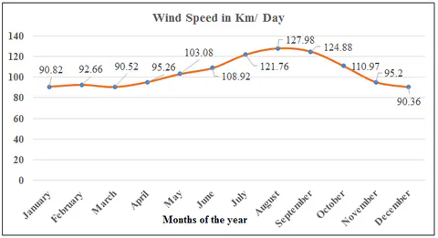
Figure 7 pertained to variation of wind speed within the period of 30 years. Based on the results plotted on Figure 7 shown above. The study findings revealed that the highest wind speed was recorded in the months of August and September with 127.98Km/day and 124.88Km/day followed by 121.76Km/day recorded in July. There was the lowest wind speed was recorded in January and December with of 90.52 km/day and 90.82 km/day for the months of March and January. The twelve monthly wind speed was calculated and found to be 104.37Km/day. The difference between maximum and minimum wind speed is only 37.62Km/day. The statistical findings showed that there is too much appreciable difference in wind speed throughout the year.
The study of Sun shine duration at the experimental site
The weather data collected from Rwanda Metrological station agency about the sun shine duration for 30 years was analyzed. The mean monthly sun shine duration for daily data was recorded originally in hours the then allow to work out the solar radiation in MJ/m2/day. The results of the average mean monthly sun shine duration expressed in percentage were plotted in a graph for the twelve months and is presented in figure 8.
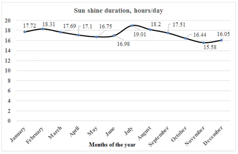
Referring to the results presented to Figure 8 shown above, it was found that the highest sunshine duration was recorded in the months of July and February with 19.1hous/day and 18.3 hours/ day which was also followed by August containing 18.2 hours/day respectively. The results also indicated that there was the lowest sunshine duration recorded in the months of November and December with of 15.58hours/ day and 16.05 hours/day respectively. The twelve monthly average sunshine hours was calculated and found to be 17.28 hours/day. The range of sunshine duration in a day varies from 15.58 to 19.1 hours/day. The difference between maximum and minimum sunshine hours is only 3.52 hours. It indicates that there is a difference of sunshine hours during rainy and dry season which resulted solar radiation ranging from 32.2 MJ/m2/day to 37.5 MJ/m2/day with the average twelve monthly solar radiation of 34.9 MJ/m2/day (See list of appendix).
To study the soil properties at the experimental site
Data related to soil physical properties were analyzed from Huye soil Lab. The soil characteristics estimated are 1) soil texture 2) bulk density of soil 3) soil porosity 4) Soil moisture content and 5) soil organic matter. These soil characteristics play an important role in the evaluation of drip irrigation performance and assessment of water use efficiency at IPRC Gishari farm as the case of interest.
Determination of Soil physical properties of the experimental site
The collected soil samples from 4 experimental plots (Plots I, II, III and IV) divided into 3 subplots (A, B and C) were transferred to Huye soil Laboratory to determine the soil physical properties including Sand (%), Silt (%) and Clay (%) respectively. The summary of statistical findings are shown in Table 6.
Determination of soil textural based on usda triangle at the experimental site
Soil texture is one of the important characteristics of soil profile. It is a physical property needed to be studied when evaluating the performance of drip irrigation on any crop in the field. It describes the proportion of Sand (%), Silt (%) and Clay (%) respectively. Soil samples were collected in the selected experimental site at IPRC Gishari farm and was arranged in such way that all plots (Plots I, II, III and IV) were divided into 3 subplots (A, B and C) to form the total area of 120 m x 64 m=7680 m2 0r 0.768ha of cropped land with carrot under drip irrigation system. The details about the statistical findings are summarized given below.
| Plot No | stats | Sand % | Silt % | Clay % | Soil Texture based on USDA |
|---|---|---|---|---|---|
| Plot I | Mean | 70.619 | 22.653 | 6.728 | Sandy Loam Soil |
| P50 | 70.382 | 22.623 | 5.194 | ||
| SD | 1.460 | 4.494 | 5.212 | ||
| Min | 69.291 | 18.174 | 2.456 | ||
| Max | 72.183 | 27.162 | 12.535 | ||
| CV | 0.021 | 0.198 | 0.775 | ||
| Sum | 211.856 | 67.959 | 20.185 | ||
| N | 3 | 3 | 3 | ||
| Plot II | Mean | 68.731 | 21.268 | 10.002 | Sandy Loam Soil |
| P50 | 68.175 | 22.415 | 10.474 | ||
| SD | 2.306 | 2.627 | 1.142 | ||
| Min | 66.753 | 18.262 | 8.699 | ||
| Max | 71.264 | 23.126 | 10.832 | ||
| CV | 0.034 | 0.124 | 0.114 | ||
| Sum | 206.192 | 63.803 | 30.005 | ||
| N | 3 | 3 | 3 | ||
| Plot III | Mean | 68.864 | 19.146 | 11.990 | Sandy Loam Soil |
| P50 | 69.184 | 19.015 | 11.801 | ||
| variance | 2.261 | 3.819 | 0.250 | ||
| SD | 1.504 | 1.954 | 0.500 | ||
| Min | 67.226 | 17.261 | 11.611 | ||
| Max | 70.182 | 21.163 | 12.557 | ||
| CV | 0.022 | 0.102 | 0.042 | ||
| Sum | 206.592 | 57.439 | 35.969 | ||
| N | 3 | 3 | 3 | ||
| Plot IV | Mean | 64.414 | 26.631 | 8.955 | Sandy Loam Soil |
| P50 | 64.163 | 27.417 | 7.181 | ||
| SD | 1.859 | 3.947 | 3.955 | ||
| Min | 62.693 | 22.351 | 6.197 | ||
| Max | 66.386 | 30.126 | 13.486 | ||
| CV | 0.029 | 0.148 | 0.442 | ||
| Sum | 193.242 | 79.894 | 26.864 | ||
| N | 3 | 3 | 3 | ||
| Total of the experimental site | Mean | 68.157 | 22.425 | 9.419 | Sandy Loam Soil |
| P50 | 68.680 | 22.383 | 10.653 | ||
| SD | 2.845 | 4.073 | 3.463 | ||
| Min | 62.693 | 17.261 | 2.456 | ||
| Max | 72.183 | 30.126 | 13.486 | ||
| CV | 0.042 | 0.182 | 0.368 | ||
| Sum | 817.882 | 269.095 | 113.023 | ||
| N | 12 | 12 | 12 |
Table 6 revealed that the all soil plots of the experimental site (plot I to plot IV) is having the texture of sandy loam soil. The average values of sand, silt and clay among the four plots were 68%, 22% and 9% respectively for the whole experimented farm under drip irrigation system for carrot production. The texture triangle for the averages of four plots shows that the soil as sandy loam soil.
Determination of soil Bulk Density (bd) of the experimental site
The representative soil samples were taken from the four experimental plots (plot I to plot IV). Its weight and volume were determined. Then the soil bulk density was found by calculating the dry mass divided by the total volume. Table 7 shows the bulk density of the soil in the selected sampled plots.
| Plot No | stats | W1 | Area, cm2 | H, cm | Oven dry weight | Volume, m3 | BD, gm/cm3 |
|---|---|---|---|---|---|---|---|
| Plot I | Mean | 200 | 47.607 | 5.167 | 137.160 | 245.971 | 0.815 |
| P50 (Median) | 200 | 47.607 | 5.100 | 139.700 | 242.797 | 0.824 | |
| SD | 0.000 | 0.000 | 0.306 | 10.483 | 14.544 | 0.047 | |
| Min | 200 | 47.607 | 4.900 | 125.640 | 233.276 | 0.764 | |
| Max | 200 | 47.607 | 5.500 | 146.140 | 261.840 | 0.857 | |
| CV | 0.000 | 0.000 | 0.059 | 0.076 | 0.059 | 0.058 | |
| N (Obs) | 3 | 3 | 3 | 3 | 3 | 3 | |
| Plot II | Mean | 200 | 47.607 | 3.500 | 123.550 | 166.626 | 1.276 |
| P50 (Median) | 200 | 47.607 | 3.400 | 122.140 | 161.865 | 1.236 | |
| SD | 0.000 | 0.000 | 1.054 | 5.629 | 50.157 | 0.385 | |
| Min | 200 | 47.607 | 2.500 | 118.760 | 119.018 | 0.913 | |
| Max | 200 | 47.607 | 4.600 | 129.750 | 218.994 | 1.680 | |
| CV | 0.000 | 0.000 | 0.301 | 0.046 | 0.301 | 0.302 | |
| N (Obs) | 3 | 3 | 3 | 3 | 3 | 3 | |
| Plot III | Mean | 200 | 47.607 | 6.500 | 135.357 | 309.447 | 0.651 |
| P50 (Median) | 200 | 47.607 | 6.600 | 132.130 | 314.208 | 0.637 | |
| SD | 0 | 0.000 | 0.656 | 7.677 | 31.218 | 0.067 | |
| Min | 200 | 47.607 | 5.800 | 129.820 | 276.122 | 0.592 | |
| Max | 200 | 47.607 | 7.100 | 144.120 | 338.012 | 0.724 | |
| CV | 0.000 | 0.000 | 0.101 | 0.057 | 0.101 | 0.104 | |
| N (Obs) | 3 | 3 | 3 | 3 | 3 | 3 | |
| Plot IV | Mean | 200 | 47.607 | 8.000 | 128.660 | 380.858 | 0.531 |
| P50 (Median) | 200 | 47.607 | 8.400 | 128.120 | 399.901 | 0.500 | |
| SD | 0.000 | 0.000 | 0.964 | 3.819 | 45.911 | 0.068 | |
| Min | 200 | 47.607 | 6.900 | 125.140 | 328.490 | 0.483 | |
| Max | 200 | 47.607 | 8.700 | 132.720 | 414.184 | 0.609 | |
| CV | 0.000 | 0.000 | 0.121 | 0.030 | 0.121 | 0.129 | |
| Sum | 600 | 142.822 | 24.000 | 385.980 | 1142.575 | 1.592 | |
| N (Obs) | 3 | 3 | 3 | 3 | 3 | 3 | |
| Total of the experimental site | Mean | 200 | 47.607 | 5.792 | 131.182 | 275.726 | 0.818 |
| SD | 0.000 | 0.000 | 1.863 | 8.440 | 88.705 | 0.341 | |
| Min | 200 | 47.607 | 2.500 | 118.760 | 119.018 | 0.483 | |
| Max | 200 | 47.607 | 8.700 | 146.140 | 414.184 | 1.680 | |
| CV | 0.000 | 0.000 | 0.322 | 0.064 | 0.322 | 0.417 | |
| N (Obs) | 12 | 12 | 12 | 12 | 12 | 12 |
Table 7 shows that the average bulk density of the soil at the first experimental plot was 0.815 gm/cm3. It was also found out that the average bulk density of the soil at the second, third and fourth experimental plots were 1.276 gm/cm3, 0.651 gm/cm3, and 0.531 gm/cm3 respectively. The overall bulk density of the soil was found to be 0.818 gm/cm3 from plot I to plot IV of the experimental site located at IPRC Gishari farm.
Determination of soil Porosity of the experimental site
The representative soil samples were taken from the four experimental site of IPRC Gishari farm. It is put inside of a graduated beaker and its volume is noted. Another graduated beaker is taken with water. Its initial volume of water is noted. Then find out the volume of water added to the soil. Soil porosity is the ratio of volume of air present in the soil (water added to the soil) to the total volume of the soil expressed in percentage.
| Plot No | Stats | W0 | W1 | W2 | W3 | W4 | Porosity (%) |
|---|---|---|---|---|---|---|---|
| Plot I | Mean | 200 | 137.160 | 337.160 | 372.587 | 35.427 | 9.496 |
| P50 | 200 | 139.700 | 339.700 | 373.020 | 36.120 | 9.611 | |
| SD | 000 | 10.483 | 10.483 | 3.470 | 12.315 | 3.265 | |
| Min | 200 | 125.640 | 325.640 | 368.920 | 22.780 | 6.175 | |
| Max | 200 | 146.140 | 346.140 | 375.820 | 47.380 | 12.702 | |
| CV | 000 | 0.076 | 0.031 | 0.009 | 0.348 | 0.344 | |
| Sum | 600 | 411.480 | 1011.480 | 1117.760 | 106.280 | 28.487 | |
| N | 3 | 3 | 3 | 3 | 3 | 3 | |
| Plot II | Mean | 200 | 125.220 | 325.220 | 380.797 | 55.577 | 14.592 |
| P50 | 200 | 127.150 | 327.150 | 381.180 | 55.140 | 14.424 | |
| SD | 000 | 5.744 | 5.744 | 1.717 | 6.636 | 1.706 | |
| Min | 200 | 118.760 | 318.760 | 378.920 | 49.170 | 12.976 | |
| Max | 200 | 129.750 | 329.750 | 382.290 | 62.420 | 16.375 | |
| CV | 000 | 0.046 | 0.018 | 0.005 | 0.119 | 0.117 | |
| Sum | 600 | 375.660 | 975.660 | 1142.390 | 166.730 | 43.775 | |
| N | 3 | 3 | 3 | 3 | 3 | 3 | |
| Plot III | Mean | 200 | 131.293 | 331.293 | 384.180 | 52.887 | 13.734 |
| P50 | 200 | 134.280 | 334.280 | 386.640 | 52.610 | 14.503 | |
| SD | 000 | 19.829 | 19.829 | 20.312 | 15.847 | 3.792 | |
| Min | 200 | 110.140 | 310.140 | 362.750 | 37.180 | 9.616 | |
| Max | 200 | 149.460 | 349.460 | 403.150 | 68.870 | 17.083 | |
| CV | 000 | 0.151 | 0.060 | 0.053 | 0.300 | 0.276 | |
| Sum | 600 | 393.880 | 993.880 | 1152.540 | 158.660 | 41.202 | |
| N | 3 | 3 | 3 | 3 | 3 | 3 | |
| Plot IV | Mean | 200 | 131.990 | 331.990 | 375.097 | 43.107 | 11.460 |
| P50 | 200 | 131.420 | 331.420 | 373.570 | 42.150 | 11.283 | |
| SD | 000 | 4.045 | 4.045 | 6.810 | 10.727 | 2.645 | |
| Min | 200 | 128.260 | 328.260 | 369.180 | 32.890 | 8.909 | |
| Max | 200 | 136.290 | 336.290 | 382.540 | 54.280 | 14.189 | |
| CV | 000 | 0.031 | 0.012 | 0.018 | 0.249 | 0.231 | |
| Sum | 600 | 395.970 | 995.970 | 1125.290 | 129.320 | 34.381 | |
| N | 3 | 3 | 3 | 3 | 3 | 3 | |
| Total of the site | Mean | 200 | 131.416 | 331.416 | 378.165 | 46.749 | 12.321 |
| P50 | 200 | 130.585 | 330.585 | 377.370 | 48.275 | 12.839 | |
| SD | 000 | 10.955 | 10.955 | 10.439 | 13.125 | 3.269 | |
| Min | 200 | 110.140 | 310.140 | 362.750 | 22.780 | 6.175 | |
| Max | 200 | 149.460 | 349.460 | 403.150 | 68.870 | 17.083 | |
| CV | 000 | 0.083 | 0.033 | 0.028 | 0.281 | 0.265 | |
| Sum | 2400 | 1576.990 | 3976.990 | 4537.980 | 560.990 | 147.847 | |
| N | 12 | 12 | 12 | 12 | 12 | 12 |
W0: Weight of beaker, W1: Weight of Dry soil, W2: Weight of beaker + Dry soil, W3: Weight of beaker, Dry soil and added water up to Field Capacity (FC), W4: Weight of Water/ Voids space, W4 = (W3-W2) and Porosity (W3-W2)/ W3 * (100)
Table 8 shows that the average soil porosity of the soil at the first experimental soil plot was 9.496%. It was also found out that the average soil porosity at the second, third and fourth experimental plots were 14.59%, 13.73% and 11.46% respectively. The overall total soil porosity of the soil was found to be 12.32% from plot I to plot IV of the experimental site located at IPRC Gishari farm.
Comparison of studied soil bd based on usda triangle
The Soil Quality Kit guidelines given by the USDA, Natural Resources Conservation Services was used to compare the soil texture of the experimental plots from IPRC Gishari farm and the soil bulk densities computed for different experimental four (4) plots of soils. The comparisons are given and discussed below:
| Plots | Soil texture | Bulk Density (BD) of experimental plots, gm/cm3 | USDA-NRCS guidelines Bulk Density (BD) in, gm/cm3 and soil texture | Decision taken while comparison | |||
|---|---|---|---|---|---|---|---|
| Range of Soil Bulk Density | Average Bulk Density | Ideal BD for plant growth | BD that affect root growth | BD that restrict root growth | |||
| Plot I | Sandy loam soil | 0.764 to 0.857 | 0.815 | < 1.40 | 1.63 | > 1.80 | Bulk density of 0.815 gm/cm3 is ideal for plant growth |
| Plot II | Sandy loam soil | 0.913 to 1.68 | 1.276 | < 1.40 | 1.60 | > 1.75 | Bulk density of 1.276 gm/cm3 ideal for plant growth |
| Plot III | Sandy loam soil | 0.592 to 0.724 | 0.651 | < 1.40 | 1.60 | > 1.75 | Bulk density of 0.651 gm/cm3 is ideal for plant growth |
| Plot IV | Sandy loam soil | 0.483 to 0.609 | 0.531 | < 1.40 | 1.60 | > 1.75 | Bulk density of 0.531 gm/cm3 is ideal for plant growth |
| All plots | Sandy Loam | 0.483 to 1.68 | 0.818 | < 1.40 | 1.60 | > 1.75 | Bulk density of 0.531 gm/cm3 is ideal for plant growth |
Table 9 shows that the comparison of soil texture and soil bulk density as per the USDA-NRCS guidelines. It was found that the all experimental plots from plot I to plot IV are ideal for plant growth because their bulk densities are always lesser or almost equal compared to the prescribed bulk densities for ideal plant growth and the soil texture varies from sandy loam by USDA triangle. It showed that all experimental site from IPRC Gishari farm has no restriction for plant growth.
Determination of Soil Moisture and Soil organic matter of the experimental site
Different soil physical properties like Soil moisture content (MC) and Soil Organic Matter (SOM) were determined. The moisture content of soil helps to determine the quantity of water removed from the soil while SOM helps to improve the soil structure, aggregation and water retention. SOM contributes to nutrient retention and turnover, soil structure, moisture retention and availability and degradation of pollutants. The Table 10 shows the summary of descriptive statistics of soil MC and SOM from the all experimental plots.
| Plot No | Stats | W1 | W2 | MC (%) | K, grs | W3, grs | W4, grs | SOM (%) |
|---|---|---|---|---|---|---|---|---|
| Plot I | Mean | 10 | 6.030 | 39.700 | 33.243 | 39.273 | 25.320 | 36.028 |
| P50 (Median) | 10 | 5.620 | 43.800 | 32.820 | 38.440 | 22.160 | 42.352 | |
| SD | 0 | 2.145 | 21.446 | 0.768 | 1.611 | 8.436 | 18.499 | |
| Min | 10 | 4.120 | 16.500 | 32.780 | 38.250 | 18.920 | 15.196 | |
| Max | 10 | 8.350 | 58.800 | 34.130 | 41.130 | 34.880 | 50.536 | |
| CV | 0 | 0.356 | 0.540 | 0.023 | 0.041 | 0.333 | 0.513 | |
| N | 3 | 3 | 3 | 3 | 3 | 3 | 3 | |
| Plot II | Mean | 10 | 6.777 | 32.233 | 33.853 | 40.630 | 33.983 | 16.098 |
| P50 (Median) | 10 | 6.920 | 30.800 | 35.290 | 41.470 | 32.870 | 11.995 | |
| SD | 0 | 0.539 | 5.395 | 3.262 | 2.951 | 2.586 | 8.053 | |
| Min | 10 | 6.180 | 27.700 | 30.120 | 37.350 | 32.140 | 10.924 | |
| Max | 10 | 7.230 | 38.200 | 36.150 | 43.070 | 36.940 | 25.377 | |
| CV | 0 | 0.080 | 0.167 | 0.096 | 0.073 | 0.076 | 0.500 | |
| N | 3 | 3 | 3 | 3 | 3 | 3 | 3 | |
| Plot III | Mean | 10 | 5.887 | 41.133 | 31.733 | 37.620 | 28.727 | 23.870 |
| P50 (Median) | 10 | 5.840 | 41.600 | 31.870 | 38.710 | 29.280 | 24.942 | |
| SD | 0 | 0.931 | 9.309 | 1.510 | 2.153 | 4.307 | 7.939 | |
| Min | 10 | 4.980 | 31.600 | 30.160 | 35.140 | 24.170 | 15.448 | |
| Max | 10 | 6.840 | 50.200 | 33.170 | 39.010 | 32.730 | 31.218 | |
| CV | 0 | 0.158 | 0.226 | 0.048 | 0.057 | 0.150 | 0.333 | |
| N | 3 | 3 | 3 | 3 | 3 | 3 | 3 | |
| Plot IV | Mean | 10 | 6.407 | 35.933 | 32.823 | 39.230 | 29.910 | 23.778 |
| P50 (Median) | 10 | 6.290 | 37.100 | 32.810 | 40.180 | 28.750 | 24.144 | |
| SD | 0 | 0.911 | 9.106 | 2.050 | 1.875 | 2.574 | 4.862 | |
| Min | 10 | 5.560 | 26.300 | 30.780 | 37.070 | 28.120 | 18.744 | |
| Max | 10 | 7.370 | 44.400 | 34.880 | 40.440 | 32.860 | 28.447 | |
| CV | 0 | 0.142 | 0.253 | 0.062 | 0.048 | 0.086 | 0.204 | |
| N | 3 | 3 | 3 | 3 | 3 | 3 | 3 | |
| Total | Mean | 10 | 6.275 | 37.250 | 32.913 | 39.188 | 29.485 | 24.943 |
| P50 (Median) | 10 | 6.235 | 37.650 | 32.815 | 38.860 | 30.710 | 24.543 | |
| SD | 0 | 1.153 | 11.525 | 1.968 | 2.186 | 5.403 | 12.054 | |
| Min | 10 | 4.120 | 16.500 | 30.120 | 35.140 | 18.920 | 10.924 | |
| Max | 10 | 8.350 | 58.800 | 36.150 | 43.070 | 36.940 | 50.536 | |
| CV | 0 | 0.184 | 0.309 | 0.060 | 0.056 | 0.183 | 0.483 | |
| N | 12 | 12 | 12 | 12 | 12 | 12 | 12 |
W1 = Initial weight of the soil; W2 = Weight of the soil after drying (gms); MC = (W2−W1/W1)×100; K (gms) = Weight of crucibles; W3 = Weight of Crucibles + Dried soil @105°C; W4 = Weight of Crucibles + Dried soil @450°C.
Table 10 pertained to soil MC and SOM for all the sampled plots from the experimental site. The MC from the all plots varies from 16.5% to 58.8% while the average mean MC was found to be 37.25% of H2O was removed and evaporated. Soil Organic Matter (SOM) was evaluated when heating the soil samples contained in weighted crucibles from 105ºC to 450ºC and above not higher than 800ºC for the period between 6hours and 8hours. The study findings also showed that SOM for all experimental plots varies from 10.92% to 50.54% while the overall average mean SOM was found to be 24.94% respectively. These findings agree with the research conducted by (R. Wang, Kang, & Wan, 2015) who find that SOM is higher on the top soil and is reducing through intensive irrigation
Determination of soil chemical properties of the experimental site
The sampled soil samples were collected and transported in plastics and thereafter transferred to Huye soil Laboratory for chemical analysis. The soil tests conducted was mainly focused on determination of soil chemical properties like Ca, Mg, Na, K and nitrogen only. The soil samples also were analyzed to determine the soil acidity (pH) with pH 7.0 buffer solution of KCL, soil salinity (Electrical conductivity or EC) and Sodium Adsorption Ratio (SAR) of the soil respectively.
Determination of soil chemical properties (Ca, Mg, Na, K, and N)
The soil samples were taken from different 4 soil plots form the experimental site of the IPRC Gishari farm. The soil samples were taken from different subplots (subplots A, B and C) and then the summary of statistical findings are shown for soil chemical properties are presented in Table 11 below.
| Plot No | Stats | Ca | Mg | Na | K | N | T0C |
|---|---|---|---|---|---|---|---|
| Plot I | Mean | 0.919 | 1.471 | 1.101 | 0.652 | 2.157 | 28.133 |
| P50 (Median) | 0.883 | 1.937 | 1.128 | 0.669 | 2.163 | 28.580 | |
| Variance | 0.025 | 1.057 | 0.014 | 0.030 | 0.043 | 3.108 | |
| SD | 0.158 | 1.028 | 0.116 | 0.173 | 0.207 | 1.763 | |
| Min | 0.782 | 0.292 | 0.973 | 0.472 | 1.947 | 26.190 | |
| Max | 1.092 | 2.183 | 1.201 | 0.816 | 2.361 | 29.630 | |
| CV | 0.172 | 0.699 | 0.106 | 0.265 | 0.096 | 0.063 | |
| Sum | 2.757 | 4.412 | 3.302 | 1.957 | 6.471 | 84.400 | |
| N | 3 | 3 | 3 | 3 | 3 | 3 | |
| Plot II | Mean | 0.919 | 1.860 | 1.087 | 0.713 | 1.219 | 28.353 |
| P50 (Median) | 0.937 | 1.911 | 1.173 | 0.729 | 0.972 | 28.520 | |
| Variance | 0.038 | 0.045 | 0.039 | 0.104 | 0.399 | 0.849 | |
| SD | 0.194 | 0.212 | 0.197 | 0.323 | 0.631 | 0.921 | |
| Min | 0.716 | 1.628 | 0.862 | 0.382 | 0.749 | 27.360 | |
| Max | 1.103 | 2.042 | 1.227 | 1.027 | 1.937 | 29.180 | |
| CV | 0.211 | 0.114 | 0.181 | 0.453 | 0.518 | 0.032 | |
| Sum | 2.756 | 5.581 | 3.262 | 2.138 | 3.658 | 85.060 | |
| N | 3 | 3 | 3 | 3 | 3 | 3 | |
| Plot III | Mean | 0.845 | 1.758 | 1.052 | 1.105 | 2.027 | 28.770 |
| P50 (Median) | 0.826 | 1.451 | 1.042 | 1.182 | 2.172 | 28.930 | |
| Variance | 0.002 | 0.412 | 0.006 | 0.046 | 0.792 | 0.404 | |
| SD | 0.041 | 0.642 | 0.076 | 0.215 | 0.890 | 0.635 | |
| Min | 0.817 | 1.328 | 0.981 | 0.862 | 1.073 | 28.070 | |
| Max | 0.892 | 2.496 | 1.132 | 1.271 | 2.835 | 29.310 | |
| CV | 0.048 | 0.365 | 0.072 | 0.195 | 0.439 | 0.022 | |
| Sum | 2.535 | 5.275 | 3.155 | 3.315 | 6.080 | 86.310 | |
| N | 3 | 3 | 3 | 3 | 3 | 3 | |
| Plot IV | Mean | 0.923 | 1.254 | 0.950 | 0.734 | 1.680 | 28.547 |
| P50 (Median) | 1.012 | 1.072 | 0.962 | 0.627 | 1.892 | 28.620 | |
| Variance | 0.026 | 0.259 | 0.035 | 0.183 | 0.381 | 0.453 | |
| SD | 0.163 | 0.509 | 0.186 | 0.427 | 0.618 | 0.673 | |
| Min | 0.735 | 0.862 | 0.758 | 0.371 | 0.984 | 27.840 | |
| Max | 1.021 | 1.829 | 1.129 | 1.205 | 2.163 | 29.180 | |
| CV | 0.176 | 0.405 | 0.196 | 0.582 | 0.368 | 0.024 | |
| Sum | 2.768 | 3.763 | 2.849 | 2.203 | 5.039 | 85.640 | |
| N | 3 | 3 | 3 | 3 | 3 | 3 | |
| Total | Mean | 0.901 | 1.586 | 1.047 | 0.801 | 1.771 | 28.451 |
| P50 (Median) | 0.888 | 1.729 | 1.085 | 0.773 | 1.942 | 28.600 | |
| Variance | 0.018 | 0.385 | 0.021 | 0.101 | 0.437 | 0.936 | |
| SD | 0.133 | 0.620 | 0.144 | 0.317 | 0.661 | 0.967 | |
| Min | 0.716 | 0.292 | 0.758 | 0.371 | 0.749 | 26.190 | |
| Max | 1.103 | 2.496 | 1.227 | 1.271 | 2.835 | 29.630 | |
| CV | 0.147 | 0.391 | 0.137 | 0.396 | 0.373 | 0.034 | |
| Sum | 10.816 | 19.031 | 12.568 | 9.613 | 21.248 | 341.410 | |
| N | 12 | 12 | 12 | 12 | 12 | 12 |
N.B: ppm is the part per millions or equivalent to mg/l
Table 11 reveals the fact that the calcium (Ca) content of the experimental plots (plot I to plot IV) was at 0.901 ppm, its range varies from 0.716 ppm to 1.103 ppm.The standard deviation was found to be 0.13. It means there was no appreciable change of calcium content in all four sampled plots due to the Coefficient of Variation (CV) less than 0.50 at 0.15.
For Magnesium content, the study findings presented in Table 11 showed that the concentration of Mg in the experimental plots (plot I to plot IV) was at 1.59 ppm, its range varies from 0.292 ppm to 2.496 ppm.The standard deviation was found to be 0.620. It means there was no appreciable change of Magnesium content in all four sampled plots due to the Coefficient of Variation (CV) less than 0.50 at 0.39 respectively.
Furthermore, Table 11 reveals the fact that the Sodium (Na) content of the experimental plots (plot I to plot IV) was at 1.047 ppm, its range varies from 0.758 ppm to 1.227 ppm.The standard deviation was found to be 0.144. It means there was no appreciable change of Sodium content in all four sampled plots due to the Coefficient of Variation (CV) less than 0.50 at 0.14 respectively.
It indicates that also Potassium (K) content of the experimental plots (plot I to plot IV) was at 0.801 ppm, its range varies from 0.371 ppm to 1.271 ppm.The standard deviation was found to be 0.317. It means there was no appreciable change of Sodium content in all four sampled plots due to the Coefficient of Variation (CV) less than 0.50 at 0.40 which is higher compared to other chemical properties studied respectively.
The Nitrogen (N) content from all four experimental plots was studied through the Titration reaction. Table 11 reveals the fact that the Nitrogen (N) content of the experimental plots (plot I to plot IV) was at 1.771 ppm, its range varies from 0.749 ppm to 2.835ppm.The standard deviation was found to be 0.661 considering the all four experimental plots. It means there was no appreciable change of Nitrogen content in all four sampled plots due to the Coefficient of Variation (CV) less than 0.50 at 0.37 respectively.
The study findings also showed that the average mean temperature was 28.5ºC and its range varies from 26.2ºC to 29.6ºC. The corresponding standard deviation was found to be 0.967. It means there was no appreciable change of soil temperature due to high moisture content in all four sampled plots; and due to the Coefficient of Variation (CV) less than 0.50 at 0.034 respectively to indicate very small variation in temperature of the soil plots.
Determination of soil acidity, salinity and alkalinity of the experimental site
The soil samples taken from the experimental site were tested for pH, EC and SAR respectively. The soil acidity was tested by finding out the soil pH. The soil salinity was tested by finding out the soil electrical conductivity (EC) and the soil alkalinity was tested by finding out the soil Sodium Adsorption Ratio (SAR). They are discussed below in Table 12.
| Plots No | Stats | pH | EC (µs/cm) | SAR |
|---|---|---|---|---|
| Plot I | Mean | 6.497 | 86.51 | 0.382 |
| P50 (Median) | 6.520 | 88.32 | 0.332 | |
| Variance | 0.042 | 50.91 | 0.015 | |
| SD | 0.206 | 7.135 | 0.121 | |
| Min | 6.280 | 78.64 | 0.295 | |
| Max | 6.690 | 92.56 | 0.520 | |
| CV | 0.032 | 0.082 | 0.316 | |
| Sum | 19.490 | 259.50 | 1.147 | |
| N | 3 | 3 | 3 | |
| Plot II | Mean | 7.033 | 69.87 | 0.330 |
| P50 (Median) | 7.150 | 70.62 | 0.340 | |
| Variance | 0.070 | 7.494 | 0.006 | |
| SD | 0.265 | 2.737 | 0.077 | |
| Min | 6.730 | 66.84 | 0.248 | |
| Max | 7.220 | 72.16 | 0.401 | |
| CV | 0.038 | 0.039 | 0.233 | |
| Sum | 21.100 | 209.60 | 0.989 | |
| N | 3 | 3 | 3 | |
| Plot III | Mean | 6.973 | 71.70 | 0.329 |
| P50 (Median) | 6.930 | 71.76 | 0.325 | |
| Variance | 0.025 | 4.690 | 4E-04 | |
| SD | 0.159 | 2.166 | 0.020 | |
| Min | 6.840 | 69.51 | 0.311 | |
| Max | 7.150 | 73.84 | 0.350 | |
| CV | 0.023 | 0.030 | 0.060 | |
| Sum | 20.920 | 215.10 | 0.986 | |
| N | 3 | 3 | 3 | |
| Plot IV | Mean | 7.217 | 68.36 | 0.322 |
| P50 (Median) | 7.240 | 68.27 | 0.333 | |
| Variance | 0.002 | 5.001 | 4E-04 | |
| SD | 0.049 | 2.236 | 0.020 | |
| Min | 7.160 | 66.17 | 0.300 | |
| Max | 7.250 | 70.64 | 0.334 | |
| CV | 0.007 | 0.033 | 0.061 | |
| Sum | 21.650 | 205.10 | 0.967 | |
| N | 3 | 3 | 3 | |
| Total of the experimental site | Mean | 6.930 | 74.11 | 0.341 |
| P50 (Median) | 7.040 | 71.20 | 0.333 | |
| Variance | 0.103 | 69.78 | 0.005 | |
| SD | 0.320 | 8.354 | 0.067 | |
| Min | 6.280 | 66.17 | 0.248 | |
| Max | 7.250 | 92.56 | 0.520 | |
| CV | 0.046 | 0.113 | 0.197 | |
| Sum | 83.160 | 889.30 | 4.089 | |
| N | 12 | 12 | 12 |
Table 12 reveals the fact that the pH value at the all experimental plots (plot I to plot IV) is 6.9, its range varies from 6.3 to 7.3 which is acidic and the pH changes from acidic to alkaline soil as it is nearing the neutral soil of pH 7. The conclusion is the soil had acidic property from all experimental plots thereafter, there is slight decrease in acidity, which is nearing to neutral. Overall, the soil is acidic in nature; and partially, as far as most soils for Gishari farm fall in the range of 6.3 to 7.2 near to pH of 7.0 level which is considered neutral, the farmers from the study area are encouraged to grow some acid-tolerant plants which could with stand to very strong, medium and very slightly to neutral pH to increase crop productivity at farmer level. Normally, the soil pH behaves oppositely with the SOM in nature; when the SOM is higher on the top soil, it should reduce the pH respectively. Thus these results agree with the research conducted by Van Bergeijk, Noordijk, Lembrechts, and Frissel (1992) who found similar results
Table 12 reveals the fact that the EC (µS/cm) value at the all experimental plots (plot I to plot IV) is 74.11 µS/cm, its range varies from 66.17 µS/cm to 92.56 µS/cm which is saline soil. The plant growth is affected by salt availability in all experimental plots and this should be reduced by leaching through drip irrigation system. According to Abrol, Yadav, & Massoud (1988), the soils having EC range of 20-40 µS/cm is considered to be slightly saline soils, the soils having the EC range of 40-80 µS/cm is considered to be moderate saline soils and the soils having the EC greater than 80 µS/cm are considered to be strong saline soils. The strong saline soils need to be cultivated with crops tolerance to saline soils for increased crop productivity. Considering the overall soil sample from the four experimental plots (plot I to plot IV), the EC has the value of 74.11 µS/cm and hence the soil of IPRC Gishari farm is called “ Moderate saline soil” as per the classification made by Abrol et al. (1988) respectively.
Furthermore, Table 12 reveals the fact that the SAR at the all experimental soil plots (plot I to plots IV) cm is 0.341which is lower. The SAR for the whole experimented farm was in range of 0.248 to 0.52 respectively. The standard deviation of the SAR was found to be 0.067. The coefficient of variation (CV) for the whole experimental plots was found to be 0.197 which is very small compared to 0.50 as reference. There is an indication that the SAR depth of the soil is fluctuating slowly within the farm. The results from the field measurement concluded that the SAR of the soil from IPRC Gishari farm do not falls in permissible limits of 0 - 0.3 set by (FAO, 1992) and Waller and Yitayew (2015) which are acceptable for plant growth. There is need to undertake soil reclamation to bring back this soil to normal condition that favour plant grow.
Analysis of Variance of soil physical and chemical properties of the experimental site
The Analysis of Variance of samples soil samples was performed to indicate the significance of soil physical variability of the experimental site. The Duncan test was used to indicate the significance levels at 5% level of significance of the experimental plots.
Analysis of Variance (anova) of soil physical properties
The Analysis of Variance (ANOVA) one way of soil samples was performed through Duncan test to indicate the variability of soil physical properties like sand (%), silt (%), clay (%), Bulk Density (g/cm3), Soil porosity (%), MC (%) and SOM (%) by plots at 5% level of significance. The degree of freedom (DF), calculated F and the p-value were taken into consideration to explain the factor that have fluctuated over experimental plots. The results from ANOVA one-way are shown in the Table 13 below.
| Parameters | Source of Variation | Sum of Squares | Df | Mean Square | F | Sig. |
|---|---|---|---|---|---|---|
| Sand % | Between Groups | 62.7 | 3 | 20.9 | 6.347 | 0.016** |
| Within Groups | 26.34 | 8 | 3.292 | |||
| Total | 89.04 | 11 | ||||
| Silt % | Between Groups | 89.5 | 3 | 29.83 | 2.567 | 0.127 ns |
| Within Groups | 92.99 | 8 | 11.62 | |||
| Total | 182.5 | 11 | ||||
| Clay % | Between Groups | 43.21 | 3 | 14.4 | 1.299 | 0.34 ns |
| Within Groups | 88.72 | 8 | 11.09 | |||
| Total | 131.9 | 11 | ||||
| BD, gm/cm3 | Between Groups | 0.962 | 3 | 0.321 | 8.026 | 0.009** |
| Within Groups | 0.32 | 8 | 0.04 | |||
| Total | 1.282 | 11 | ||||
| Porosity (%) | Between Groups | 47.63 | 3 | 15.88 | 1.817 | 0.222 ns |
| Within Groups | 69.89 | 8 | 8.737 | |||
| Total | 117.5 | 11 | ||||
| MC (%) | Between Groups | 144 | 3 | 47.98 | 0.291 | 0.831 ns |
| Within Groups | 1317 | 8 | 164.7 | |||
| Total | 1461 | 11 | ||||
| SOM (%) | Between Groups | 610.8 | 3 | 203.6 | 1.649 | 0.254 ns |
| Within Groups | 987.5 | 8 | 123.4 | |||
| Total | 1598 | 11 |
Note: (**) corresponds to 5% level of significance and ns means not significant
After arrangement of needed parameters by fixing depend list (soil physical properties like soil texture, bulk density, soil porosity, MC (%) and SOM (%)) and fixed factor (plots number), the researcher undertaken the ANOVA through post hoc multiple comparison of the Equal variance options via SPSS 22.0. Then the Duncan test was performed to compare the statistical significance change at 5% level of significance. Difference in parameters among experimental plots were tested by one way ANOVA. The results from one way ANOVA presented in Table 13 indicated research outputs between and within groups (plots) by showing the source of variation, sum squares (SS), degree of freedom (DF), Mean square (MS), F and sig. which is p-value. The ANOVA results from the table above showed that there was no statistically significant difference in mean plots of silt (p=0.127), clay (p=0.34), porosity (p=0.222), MC (p=0.831) and SOM (p=0.254) which are higher than 5% level of significance. Nevertheless, there were sand (%) and BD (gm/cm3) that are statistically significant differences between plots levels (p<0.05). The results from Duncan test through one way ANOVA showed that only two physical properties including sand % and BD are statistically significant at 5% level. It showed that sand % with p-value =0.016<0.05 and BD with p-value =0.009<0.05 level of probability are statistically significant changing within and between experimental plots.
Analysis of Variance (anova) of soil chemical properties of the experimental plots
The Analysis of Variance (ANOVA) one way of soil samples was performed through Duncan test to indicate the variability of soil chemical properties like Ca, Mg, Na, K and N by plots at 5% level of significance. The degree of freedom (DF), calculated F and the p-value were taken into consideration to explain the factor that have fluctuated over experimental plots. The results from ANOVA one-way are shown in the Table 14 below.
| Parameters | Source of Variation | Sum of Squares | Df | Mean Square | F | Sig. |
|---|---|---|---|---|---|---|
| Ca (ppm) | Between Groups | 0.013 | 3 | 0.004 | 0.187 | 0.902 ns |
| Within Groups | 0.182 | 8 | 0.023 | |||
| Total | 0.194 | 11 | ||||
| Mg (ppm) | Between Groups | 0.685 | 3 | 0.228 | 0.515 | 0.683 ns |
| Within Groups | 3.545 | 8 | 0.443 | |||
| Total | 4.23 | 11 | ||||
| Na (ppm) | Between Groups | 0.042 | 3 | 0.014 | 0.604 | 0.63 ns |
| Within Groups | 0.185 | 8 | 0.023 | |||
| Total | 0.227 | 11 | ||||
| K (ppm) | Between Groups | 0.38 | 3 | 0.127 | 1.398 | 0.313 ns |
| Within Groups | 0.726 | 8 | 0.091 | |||
| Total | 1.106 | 11 | ||||
| N (ppm) | Between Groups | 1.581 | 3 | 0.527 | 1.305 | 0.338 ns |
| Within Groups | 3.23 | 8 | 0.404 | |||
| Total | 4.811 | 11 | ||||
| TºC | Between Groups | 0.664 | 3 | 0.221 | 0.184 | 0.904 ns |
| Within Groups | 9.627 | 8 | 1.203 | |||
| Total | 10.29 | 11 |
Note: (**) corresponds to 5% level of significance and ns means not significant
After arrangement of needed parameters by fixing depend list (soil chemical properties like Calcium, Magnesium, Sodium, Potassium, Nitrogen and TºC) and fixed factor (plots number), the researcher undertaken the ANOVA through post hoc multiple comparison of the Equal variance options via SPSS 22.0. Then the Duncan test was performed to compare the statistical significance change at 5% level of significance. Difference in parameters among experimental plots were tested by one way ANOVA. The results from one way ANOVA presented in Table 14 indicated research outputs between and within groups (plots) by showing the source of variation, sum squares (SS), degree of freedom (DF), Mean square (MS), F and sig. which is p-value. Unexpectedly, the ANOVA results from the table above showed that there was no statistically significant difference in mean plots of Ca content (p=0.902), Mg content (p=0.683), Na content (p=0.63), K content (p=0.313), N Content (p=0.338) and TºC (p=0.904) which are higher than 5% level of significance are not statistically significant changing within and between experimental plots.
ANOVA one way of soil acidity, salinity and alkalinity of the experimental plots
The Analysis of Variance (ANOVA) one way of soil samples was performed through Duncan test to indicate the variability of soil acidity (pH), soil salinity (EC) and Sodium Adsorption Ratio (SAR) by plots at 5% level of significance. The degree of freedom (DF), calculated F and the p-value were taken into consideration to explain the factor that have fluctuated over experimental plots. The results from ANOVA one-way are shown in the Table 15 below.
| Parameters | Source of Variation | Sum of Squares | Df | Mean Square | F | Sig. |
|---|---|---|---|---|---|---|
| pH (unitless) | Between Groups | 0.848 | 3 | 0.283 | 8.041 | 0.008** |
| Within Groups | 0.281 | 8 | 0.035 | |||
| Total | 1.129 | 11 | ||||
| EC (µs/cm) | Between Groups | 631.4 | 3 | 210.5 | 12.36 | 0.002** |
| Within Groups | 136.2 | 8 | 17.02 | |||
| Total | 767.6 | 11 | ||||
| SAR | Between Groups | 0.007 | 3 | 0.002 | 0.44 | 0.731 ns |
| Within Groups | 0.043 | 8 | 0.005 | |||
| Total | 0.05 | 11 |
Note: (**) corresponds to 5% level of significance and ns means not significant
After arrangement of needed parameters by fixing depend list (soil physical properties like soil acidity, soil salinity and soil alkalinity) and fixed factor (plots number), the researcher undertaken the ANOVA through post hoc multiple comparison of the Equal variance options via SPSS 22.0. Then the Duncan test was performed to compare the statistical significance change at 5% level of significance. Difference in parameters among experimental plots were tested by one way ANOVA. The results from one way ANOVA presented in Table 15 indicated research outputs between and within groups (plots) by showing the source of variation, sum squares (SS), degree of freedom (DF), Mean square (MS), F and sig. which is p-value. The ANOVA results from the table above showed that there was no statistically significant difference in mean plots of Sodium Adsorption Ratio (SAR) with (p=0.731) which is higher than 5% level of significance is statistically significant changing within and between experimental plots. Nevertheless, there were soil acidity (pH) and soil salinity (Electrical Conductivity, EC) that are statistically significant differences between plots levels (p<0.05). The results from Duncan test through one way ANOVA showed that only two physical properties including soil acidity (pH) and soil salinity (Electrical Conductivity, EC) are statistically significant at 5% level. It showed that pH with p-value =0.008<0.05 and EC with p-value =0.002<0.05 level of probability are statistically significant changing within and between experimental plots.
The asses of crop water requirement, water deficit and irrigation scheduling of carrot
The computer software CROPWAT 8.0 was developed by FAO to estimate the crop water requirements, irrigation requirements of carrots and irrigation schedule at the experimental site (IPRC Gishari farm) using the input data like climate data, rainfall, crop data and soil data. The crop water requirement was worked out and expressed in millimetre per day.
Determination of Reference Evapotranspiration (ETo) under carrot crop
Reference evapotranspiration is the evapotranspiration from a reference surface and not water surface. It is closely showing the evapotranspiration of alfalfa grass based on physical, physiological and aerodynamic parameters. The summary of findings of reference evapotranspiration (ETo) for different months is shown below:
| Months | Min Temp | Max Temp | Humidity | Wind Speed | Sun shine duration | Rad | ETo |
|---|---|---|---|---|---|---|---|
| T°C | T°C | RH (%) | km/day | Hours | MJ/m²/day | mm/day | |
| January | 15 | 26.4 | 70 | 91 | 17.7 | 35.2 | 5.94 |
| February | 15.3 | 27.2 | 67 | 93 | 18.3 | 37.5 | 6.47 |
| March | 15.3 | 26.4 | 73 | 91 | 17.7 | 37.3 | 6.43 |
| April | 15.1 | 25.4 | 80 | 95 | 17.1 | 35.5 | 6.00 |
| May | 14.8 | 25.0 | 79 | 103 | 16.8 | 33.4 | 5.53 |
| June | 13.8 | 25.6 | 69 | 109 | 17.0 | 32.6 | 5.42 |
| July | 13.2 | 26.0 | 61 | 122 | 19.0 | 35.8 | 5.94 |
| August | 14.2 | 26.8 | 61 | 128 | 18.2 | 36.3 | 6.25 |
| September | 14.9 | 26.9 | 65 | 125 | 17.5 | 36.4 | 6.39 |
| October | 15.1 | 26.3 | 70 | 111 | 16.4 | 34.5 | 6.01 |
| November | 15.0 | 25.4 | 76 | 95 | 15.6 | 32.2 | 5.46 |
| December | 14.9 | 25.7 | 74 | 90 | 16.1 | 32.3 | 5.43 |
| Average | 14.7 | 26.1 | 70 | 104 | 17.3 | 34.9 | 5.94 |
The weather data like minimum and maximum temperature in ºC, relative humidity (%), wind speed (km/h), sun shine duration in hours/ day were fed into CROPWAT 8.0 computer package. The solar radiation (MJ/m²/day) and Reference evapotranspiration (ETo) were generated automatically. The results presented in Table 16 revealed that monthly average mean of solar radiation was 34.9 MJ/m²/day while its range varies from 32.2 MJ/m²/day to 37.5 MJ/m²/day. The difference between maximum and minimum solar radiation was found to be 5.3 MJ/m²/day which is very high. This will request the farmer to supply much water to compensate water deficit. The lowest solar radiation was recorded in November while the highest solar radiation was recorded in February. In addition, Table 16 shows that the mean ETo for the IPRC Gishari farm experimental site was found to be 5.94 mm/day. Its range varies from 5.43 mm/day to 6.47 mm/day. The maximum ETo was found in the month February while the minimum was found in the month of December. The difference between maximum and minimum of ETo was found to be 1.04 mm/day.
Determination of Crop Water Requirement (cwr) of carrot
In irrigation practice, Crop water requirement is mainly a function of crop evapotranspiration which should be monitored in the mid-stages attributed to more crop water demand owing to full canopy development in addition to evaporative demand. However, in the late stage, though there is not much variation in the atmospheric demand, the transpiration rate decreases due to decrease in physiological activity of plants. The determination crop water requirement rely effectively on the total precipitation and effective rainfall. The results related to Crop Water Requirement are now shown in Table 17 below
Determination of Effective Rainfall (Eff. Rain) of the experimental site
When rainfalls, part of the rainwater goes as runoff and another part of the water percolates down ward. The remaining part of water stored in the root zone is called effective rainfall. Based on the values of ETo calculated above, the total rain and effective rainfall for different months are shown below.
| Months | ETo (mm/day) | Rain (mm) | Eff. Rain (mm) |
|---|---|---|---|
| January | 5.94 | 109.4 | 90.3 |
| February | 6.47 | 83.7 | 72.5 |
| March | 6.43 | 123.1 | 98.9 |
| April | 6 | 122.6 | 98.6 |
| May | 5.53 | 114.9 | 93.8 |
| June | 5.42 | 63.1 | 56.7 |
| July | 5.94 | 53 | 48.5 |
| August | 6.25 | 81.1 | 70.6 |
| September | 6.39 | 77 | 67.5 |
| October | 6.01 | 102.1 | 85.4 |
| November | 5.46 | 121.5 | 97.9 |
| December | 5.43 | 97.1 | 82 |
| Total | 5.94 | 1148.6 | 962.6 |
Reference evapotranspiration was computed and was to be 5.94 mm/day. Its range varies from 5.43 mm/day to 6.47 mm/day. The maximum ETo was found in the month February while the minimum was found in the month of December. The difference between maximum and minimum of ETo was found to be 1.04 mm/day. The total of rain fall (Total Water requirement) and effective rain fall (Crop Water Requirement) was found to be 1148.6mm and 962.6mm for the period of twelve months. It was also found that the maximum effective rainfall of 98.9 mm was found at the end of the month of March and the minimum effective rainfall was found to be 48.5mm during July. It shows that July is the dries month, which needs more irrigation and the high rainfall was found in the end of March with 123.1 mm.
Determination of Gross Irrigation (gi), Net Irrigation and water deficit of the experimental site
Net irrigation water requirement (NIWR) is the quantity of water necessary for crop growth. It is expressed in millimeters per year or in m3/ha per year (1 mm = 10 m3/ha). It depends on the cropping pattern and the climate. Information on irrigation efficiency is necessary to be able to transform NIWR into gross irrigation water requirement (GIWR), which is the quantity of water to be applied in reality, taking into account water losses. Multiplying GIWR by the area that is suitable for irrigation gives the total water requirement for that area. In this study water requirements are expressed in km3/year. Based on results concerning the total rainfall, the crop water requirement per dec was given as 207.1mm/dec and results are summarized in Table 18.
| Month | Decade | Stage | Kc | ETc | ETc | Eff rain | Irr. Req. |
|---|---|---|---|---|---|---|---|
| Period and development stages | coeff | mm/day | mm/dec | mm/dec | mm/dec | ||
| May | 2 | Init | 0.45 | 2.49 | 22.4 | 29.5 | 0.00 |
| May | 3 | Init | 0.45 | 2.47 | 27.2 | 28.1 | 0.00 |
| Jun | 1 | Deve | 0.56 | 3.04 | 30.4 | 22.1 | 8.30 |
| Jun | 2 | Deve | 0.75 | 4.07 | 40.7 | 17.6 | 23.10 |
| Jun | 3 | Deve | 0.95 | 5.29 | 52.9 | 17.1 | 35.80 |
| Jul | 1 | Mid | 1.03 | 5.95 | 59.5 | 16.1 | 43.40 |
| Jul | 2 | Mid | 1.03 | 6.13 | 61.3 | 14.8 | 46.50 |
| Jul | 3 | Late | 1.03 | 6.23 | 68.6 | 17.7 | 50.90 |
| Aug | 1 | Late | 0.98 | 6.05 | 60.5 | 21.8 | 38.60 |
| Aug | 2 | Late | 0.91 | 5.7 | 51.3 | 22.2 | 26.60 |
| Average | 474.7 | 207.1 | 273.2 | ||||
| NIWR = | NIWR = ∑ CWR × Si / S = ∑ Irr Req × Si / S, S is the cultivated area, ha | 273.2/0.768 = 355.73×10 = 3,557.3 m3/ha | |||||
| GIWR = | NIWR + Water Losses | 501.7/0.768 = 653.26×10 = 6,532.6 m3/ha | |||||
| Losses | GIWR − NIWR | (6,532.6 − 3,557.3) m3/ha = 2,975.3 m3/ha | |||||
Due to high wind speed observed at the experimental site, water losses called water deficit in drip irrigation system was also taken into consideration. Table 18 shows that the total irrigation water requirement for carrot production under drip irrigation for the season starting from 16 May to 19 August was found to be 273.2 mm. This low water requirement for carrot farming is mainly due to higher effective rain fall in the experimental site 16 May to 19 August was found to be 273.2 mm. It was also found out that the Net Irrigation Water Requirement (NIWR) was found to be 3,557.3m3/ha which is very low compared to Gross Irrigation Water Requirement (GIWR). As prescribed earlier, Gross Irrigation Water Requirement (GIWR) is the amount of water to be extracted (by diversion, pumping) and applied to the irrigation scheme. It includes NIWR plus water losses. The GIWR from the experimental site was found to be 6,532.6m3/ha respectively. The water deficit (water losses) accrued in drip irrigation system was found to be 2,975.3 m3/ha. There is a need to address the regional irrigation efficiency to reduce the water deficit for the installed drip irrigation system to perform perfectly.
Determination of Irrigation scheduling of the experimental site
Irrigation scheduling is essential for good water management and it deals with two classical questions related to irrigation. These are (1) how much to irrigate and (2) How often to irrigate (irrigation intervals). How often and how to irrigate is function of irrigation water needs of the crop. Generally, drips irrigation systems are designed to meet irrigation water requirement on daily or at an interval of 2-3 days. However, longer gap between irrigations is maintained in other irrigation system. In any case, irrigation interval is chosen such that crop does not suffers from water tress. The CROPWAT 8 computer package was built to work out the irrigation scheduling by keeping the irrigation efficiency of 70%. The effect of irrigation schedule is shown in Table 19 below.
| Irrigation Scheduling and Rainfall | |||||||||||
|---|---|---|---|---|---|---|---|---|---|---|---|
| Date | Day | Stage | Rain | Ks | Eta | Depl | Net Irr | Deficit | Loss | Gr. Irr | Flow |
| Irrigation scheduling | mm | fract. | % | % | mm | mm | mm | mm | L/s/ha | ||
| 16-May | 5 | Init | 0.00 | 1.00 | 100.00 | 50.00 | 10.00 | 0.00 | 0.00 | 14.20 | 0.33 |
| 21-May | 10 | Init | 0.00 | 1.00 | 100.00 | 57.00 | 12.40 | 0.00 | 0.00 | 17.80 | 0.41 |
| 1-Jun | 21 | Dev | 0.00 | 1.00 | 100.00 | 60.00 | 15.40 | 0.00 | 0.00 | 22.00 | 0.23 |
| 11-Jun | 31 | Dev | 0.00 | 1.00 | 100.00 | 55.00 | 16.20 | 0.00 | 0.00 | 23.20 | 0.27 |
| 16-Jun | 36 | Dev | 0.00 | 1.00 | 100.00 | 52.00 | 16.30 | 0.00 | 0.00 | 23.30 | 0.54 |
| 21-Jun | 41 | Dev | 0.00 | 1.00 | 100.00 | 65.00 | 21.60 | 0.00 | 0.00 | 30.80 | 0.71 |
| 26-Jun | 46 | Dev | 0.00 | 1.00 | 100.00 | 61.00 | 21.10 | 0.00 | 0.00 | 30.20 | 0.70 |
| 30-Jun | 50 | Dev | 0.00 | 1.00 | 100.00 | 58.00 | 21.10 | 0.00 | 0.00 | 30.20 | 0.87 |
| 5-Jul | 55 | Mid | 0.00 | 1.00 | 100.00 | 58.00 | 21.00 | 0.00 | 0.00 | 30.00 | 0.69 |
| 10-Jul | 60 | Mid | 0.00 | 1.00 | 100.00 | 66.00 | 23.80 | 0.00 | 0.00 | 34.00 | 0.79 |
| 15-Jul | 65 | Mid | 0.00 | 1.00 | 100.00 | 63.00 | 22.70 | 0.00 | 0.00 | 32.50 | 0.75 |
| 19-Jul | 69 | Mid | 0.00 | 1.00 | 100.00 | 51.00 | 18.40 | 0.00 | 0.00 | 26.30 | 0.76 |
| 22-Jul | 72 | Mid | 0.00 | 1.00 | 100.00 | 51.00 | 18.60 | 0.00 | 0.00 | 26.60 | 1.03 |
| 25-Jul | 75 | Mid | 0.00 | 1.00 | 100.00 | 52.00 | 18.70 | 0.00 | 0.00 | 26.70 | 1.03 |
| 29-Jul | 79 | Mid | 0.00 | 1.00 | 100.00 | 52.00 | 18.70 | 0.00 | 0.00 | 26.70 | 0.77 |
| 1-Aug | 82 | End | 0.00 | 1.00 | 100.00 | 51.00 | 18.50 | 0.00 | 0.00 | 26.40 | 1.02 |
| 5-Aug | 86 | End | 0.00 | 1.00 | 100.00 | 50.00 | 18.10 | 0.00 | 0.00 | 25.90 | 0.75 |
| 9-Aug | 90 | End | 0.00 | 1.00 | 100.00 | 50.00 | 18.10 | 0.00 | 0.00 | 25.90 | 0.75 |
| 15-Aug | 96 | End | 0.00 | 1.00 | 100.00 | 56.00 | 20.30 | 0.00 | 0.00 | 29.00 | 0.56 |
| 19-Aug | End | End | 0.00 | 1.00 | 0.00 | 32.00 | - | - | - | - | - |
| Total Irrigation requirement (16 May to 19 August) | 351 | 0.00 | 0.00 | 501.7 | 12.96 | ||||||
| Irrigation Scheduling | Quantity | Rainfall parameters | Quantity | ||||||||
| Total Irrigation | 501.60 mm | Total rainfall | 243.9 mm | ||||||||
| Total Net Irrigation | 351.10 mm | Effective rainfall | 107.9 mm | ||||||||
| Total Irrigation Losses | 0.00 mm | Total rain loss | 136 mm | ||||||||
| Actual water use by crop | 469 mm | Moist deficit at harvest | 11.4 mm | ||||||||
| Potential water by crop | 469 mm | Actual Irrigation requirement | 361 mm | ||||||||
| Efficiency Irrigation schedule | 100% | Efficiency Rain | 44.3% | ||||||||
| Deficiency Irrigation schedule | 0.00% | - | - | ||||||||
Based on the results generated from CROPWAT 8 computer package, Table 19 point out brings out the irrigation schedule by indicating the dates and corresponding gross and net irrigation. The planting of carrot started on 16 May of the year and the harvesting date was scheduled on 19 August and the total duration of the crop was 100 days. There were three stages of the crop namely initial stage, development stage, mid stage and harvesting end stage. The water stress coefficient (Ks) was assumed to be 1 and the actual evapotranspiration (ETa) was assumed as 100% during the entire cropping season.
The moisture depletion pattern during the irrigation schedule varies from 32% to 66% with an average depletion of 54.5% for the whole cropping period. The net irrigation supplied to the field varies from 10 mm to 23.8 mm with an average net irrigation requirement 18.47 mm. The total net irrigation supplied to the field was 351 mm. It was found that there was no deficit of irrigation to the crop and hence it was marked as 0 mm during the entire cropping schedule of May to August. The gross irrigation water requirement was varying from 14.2 mm to 34 mm with an average gross irrigation requirement of 26.4 mm. The Gross Irrigation requirement was found to be 501.7 mm. During the irrigation scheduling, the average flow rate of water to the field was computed and was found to be worked out to be 0.68 liter/sec/ha and is range varies from 0.33 to 0.79 liter/sec/ha respectively. Similarly, total rainfall during the season was 243.9 mm and the effective rainfall during the season of Sep to March was 107.9 mm. The total rain loss accrued in the field was found 136 mm. The computed moisture deficit at the harvesting stage was 11.4 mm. The study findings also showed that the actual irrigation requirement was found to be 361 mm while the irrigation efficiency of the modeling was 100% and the efficiency of rain was 28.7% respectively. These findings are coherent with the research conducted by (Rose et al., 2019) for water use efficiency in rice production in Muvumba P-8.
To assess the uniformity coefficient of water under drip irrigation system
When evaluating the performance of any irrigation system like drip or trickle irrigation system, the term “ Efficiency” should come which is explained broadly as the performance of a complete irrigation system or components of the system. Irrigation efficiency is defined as the ratio between the amount of water used to meet the consumptive use requirement of crop plus that necessary to maintain a favourable salt balance in the crop root zone to the total volume of water diverted, stored or pumped for irrigation. Thus, water applied by the irrigation system and not being made available to be taken up by plant roots is wasted and reduces irrigation efficiency.
Computational of emitters discharge at the experimental site
During the performance evaluation of drip irrigation system on carrot production, the researcher has primarily worked out the discharge of drippers by taking three replication within four plots (plot I to plot IV). The discharge was expressed in litre/hour. Results on the assessment of emitters discharge are summarized in Table 20 below.
| Plots No | Stats | R I | R II | R III | Average Discharge (L/h) |
|---|---|---|---|---|---|
| Plot I | Mean | 2.487 | 1.833 | 1.883 | 2.067 |
| SD | 0.335 | 0.165 | 0.573 | 0.239 | |
| Min | 2.160 | 1.650 | 1.280 | 1.800 | |
| Max | 2.830 | 1.970 | 2.420 | 2.260 | |
| CV | 0.135 | 0.090 | 0.304 | 0.115 | |
| Sum | 7.460 | 5.500 | 5.650 | 6.200 | |
| N (Obs) | 3 | 3 | 3 | 3 | |
| Plot II | Mean | 2.640 | 2.157 | 2.460 | 2.420 |
| SD | 0.347 | 0.630 | 0.248 | 0.331 | |
| Min | 2.260 | 1.730 | 2.270 | 2.130 | |
| Max | 2.940 | 2.880 | 2.740 | 2.780 | |
| CV | 0.131 | 0.292 | 0.101 | 0.137 | |
| Sum | 7.920 | 6.470 | 7.380 | 7.260 | |
| N (Obs) | 3 | 3 | 3 | 3 | |
| Plot III | Mean | 2.690 | 2.090 | 2.230 | 2.340 |
| SD | 0.395 | 0.111 | 0.272 | 0.082 | |
| Min | 2.240 | 1.970 | 1.980 | 2.270 | |
| Max | 2.980 | 2.190 | 2.520 | 2.430 | |
| CV | 0.147 | 0.053 | 0.122 | 0.035 | |
| Sum | 8.070 | 6.270 | 6.690 | 7.020 | |
| N (Obs) | 3 | 3 | 3 | 3 | |
| Plot IV | Mean | 2.323 | 2.313 | 2.160 | 2.263 |
| SD | 0.275 | 0.295 | 0.195 | 0.195 | |
| Min | 2.150 | 1.980 | 1.970 | 2.040 | |
| Max | 2.640 | 2.540 | 2.360 | 2.400 | |
| CV | 0.118 | 0.127 | 0.090 | 0.086 | |
| Sum | 6.970 | 6.940 | 6.480 | 6.790 | |
| N (Obs) | 3 | 3 | 3 | 3 | |
| Total | Mean | 2.535 | 2.098 | 2.183 | 2.273 |
| P50 (Median) | 2.555 | 1.975 | 2.230 | 2.295 | |
| Variance | 0.107 | 0.128 | 0.137 | 0.057 | |
| SD | 0.327 | 0.358 | 0.371 | 0.239 | |
| Min | 2.150 | 1.650 | 1.280 | 1.800 | |
| Max | 2.980 | 2.880 | 2.740 | 2.780 | |
| CV | 0.129 | 0.170 | 0.170 | 0.105 | |
| Sum | 30.420 | 25.180 | 26.200 | 27.270 | |
| N (Obs) | 12 | 12 | 12 | 12 |
Note: R1, R2 and R3 are the number of replications for field discharge estimation in l/h
The drip irrigation system from IPRC Gishari was fitted with the inline drippers. Three replication (R1, R2 and R3) for the estimation of discharge rate per hour was taken so as to deduct the average discharge rate for the experimental plots (plot I to plot IV). The statistical findings revealed that the average mean of emitters discharge rate was found to be 2.27 litre/h while its range varies from 1.8 to 2.78 litre/h. The standard deviation for the whole experimental plots was 0.239 while the CV was found to be 0.105 which is less that to 0.5 respectively. It means that there was no appreciable change of emitters’ discharge.
Parameters of drip irrigation performance evaluation at the experimental site
For the drip irrigation performance evaluation, the term “Irrigation Uniformity” may be involved in the analysis. Uniformity is a measure to describe evenness of water application over the length of the field. It is a statistical measure of the distribution of the applied water, which is affected by various factors like the method of irrigation, topography, infiltration characteristics as well as the hydraulic characteristics such as pressure, flow rate, etc. of the installed irrigation system. It is generally expressed using Christiansen’s coefficient of uniformity (CU), distribution uniformity (DU) and emission uniformity (EU) for drip irrigation systems. Irrigation application distributions are usually based on depths of water (volume per unit area); however, for micro irrigation systems they are usually based on emitter flow volumes because the entire land area is not typically wetted. Thus the Table 21 below pertained to the summary of descriptive statistics used when evaluating the performance of drip irrigation system at the experimental site located at IPRC Gishari farm.
| Plot No | Stats | Average Q | CUC | CV | EU or DU (%) |
|---|---|---|---|---|---|
| Plot I | N | 3 | 3 | 3 | 87.097 |
| Mean | 2.067 | 79.777 | 311.564 | ||
| SD | 0.239 | 23.595 | 384.863 | ||
| Min | 1.800 | 53.330 | 17.056 | ||
| Max | 2.260 | 98.670 | 747.034 | ||
| P25 | 1.800 | 53.330 | 17.056 | ||
| P75 | 2.260 | 98.670 | 747.034 | ||
| Plot II | N | 3 | 3 | 3 | 88.017 |
| Mean | 2.420 | 75.777 | 271.212 | ||
| SD | 0.331 | 23.404 | 228.788 | ||
| Min | 2.130 | 49.000 | 94.311 | ||
| Max | 2.780 | 92.330 | 529.584 | ||
| P25 | 2.130 | 49.000 | 94.311 | ||
| P75 | 2.780 | 92.330 | 529.584 | ||
| Plot III | N | 3 | 3 | 3 | 97.009 |
| Mean | 2.340 | 93.110 | 82.922 | ||
| SD | 0.082 | 7.907 | 93.555 | ||
| Min | 2.270 | 84.330 | 4.245 | ||
| Max | 2.430 | 99.670 | 186.370 | ||
| P25 | 2.270 | 84.330 | 4.245 | ||
| P75 | 2.430 | 99.670 | 186.370 | ||
| Plot IV | N | 3 | 3 | 3 | 90.133 |
| Mean | 2.263 | 85.333 | 192.884 | ||
| SD | 0.195 | 7.426 | 114.540 | ||
| Min | 2.040 | 77.330 | 98.272 | ||
| Max | 2.400 | 92.000 | 320.227 | ||
| P25 | 2.040 | 77.330 | 98.272 | ||
| P75 | 2.400 | 92.000 | 320.227 | ||
| Total | N | 12 | 12 | 12 | 93.949 |
| Mean | 2.273 | 83.499 | 214.645 | ||
| SD | 0.239 | 16.382 | 220.727 | ||
| Min | 1.800 | 49.000 | 4.245 | ||
| Max | 2.780 | 99.670 | 747.034 | ||
| CV | 0.105 | 0.196 | 1.028 | ||
| P25 | 2.135 | 80.830 | 76.231 | ||
| P75 | 2.375 | 93.830 | 254.983 |
CUC: Christiansen's Uniformity Coefficient in %, CV: Coefficient of Variation in % and EU: Emission Uniformity in %
Table 21 pertained to the evaluation of drip irrigation performance under carrot production at IPRC Gishari farm. The parameters undertaken were Christiansen’s Uniformity Coefficient, Coefficient of variation and Emission Uniformity all both expressed in percentage. As illustrated in the above table, the average mean of CU was found to be 83.5% while its range varies from 49% to 99.7%. The difference between the maximum and minimum CU was found 50.7% respectively. As the average mean of CU is 83.5% which is higher than 80% as prescribed by Ascough and Kiker (2002), hence the performance of the installed drip irrigation system is Excellent.
The average mean Coefficient of Variation for the system was found to be 214.6% for the experimented site. Its range varies from 4.2% to 747% while the difference between the maximum and minimum CV gives us 742.8% respectively. It means that, as per Pizarro (1996) the drippers should be classified by the standards of ASAE EP 405.1 (2003), stating that when C.V<5%: Excellent performance; (5≤C.V≤7%): Medium performance; (7≤C.V≤11%):Marginal performance, (11≤C.V≤15%): poor performance and C.V> 15%: Unacceptable. Hence, due to CV=214.6%, which is greater than 15% as ASAE EP 405.1 (2003), the emitters performance is not acceptable and rearrangement of drippers is needed for suitable performance.
Based on summary of descriptive statistics presented in Table 21 above, the average mean of EU was found to be 93.9% while its range varies from 87.1% to 97% observed in plot I and plot III respectively. The difference between the maximum and minimum EU was found 9.9% respectively. As the average mean of EU is 93.9% which is higher than 90% as prescribed by Opar (2016) the EU criteria adopted from ASAE, 1996(a) should be EU>90%:Excellent performance; 80≤EU≤90%: Good performance; 70≤EU≤80%: Fair performance and when EU< 70%: Poor performance. Hence, the average mean of EU of the drip irrigation system at IPRC Gishari farm is 93.9%, hence the performance of the installed drip irrigation system is excellent and our findings are in line with the results of (Al-Mhmdy & Al-Dulaimy, 2018).
Application efficiency for the drip irrigation system at the experimental site
Application efficiency relates to the actual storage of water in the root zone to meet the crop water needs in relation to the water applied to the field. It might be defined for individual irrigation or parts of irrigations or irrigation sets. Application efficiency includes any application losses to evaporation or seepage from surface water channels or furrows, any leaks from sprinkler or drip pipelines, percolation beneath the root zone, evaporation of droplets in the air, or runoff from the field. In case of surface irrigation evaporation losses are generally small but runoff and deep percolation are substantial. However, air losses (droplet evaporation and drift) can be very large if the sprinkler design or excessive pressure produces a high percentage of very fine droplets. Application efficiency is defined as:
Where, Ea= the application efficiency (%),Vs= the volume of water stored in root zone (m3), and Vf = the water delivered to the field or farm (m3). In addition, NIWR correspond to Net Irrigation Water Requirement while GIWR is the Gross Irrigation Water Requirement both all in m3 respectively.
Thus, EU for the drip irrigation system installed at IPRC Gishari was worked out and the results are given below:
Hence, the remaining of 100% - 54.45%= 45.55% corresponds to water losses.
Estimation of the yield of carrot under drip irrigation in experimental plots
The layout of the experimental site from IPRC Gishari farm was divided into 4 plots with 3 subplots by each plot. The twelve sub plots were undertaken to assess the variability of yield of carrot under drip irrigation in experimental plots. The experimental layout is shown in Figure 9.
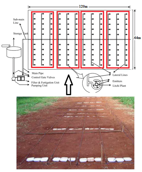
The yield of carrot was packed in plastic bags of 50Kg for easy off farm unloading and being weighted. The total area of the experimental site was 120 m x 64 m= 7680 m2 or 0.768ha of cropped land. The area of sub plots was 30 m x 16 m= 480 m2 or 0.048 ha of land. The summary of results on yield of carrot is presented in Table 22 below.
| Plot No | Stats | Farm size (Ha) | Area of plots (Ha) | Productivity (Kg/plot) |
|---|---|---|---|---|
| Plot I | Mean | 0.768 | 0.048 | 326.910 |
| P50 | 0.768 | 0.048 | 315.450 | |
| Variance | 0.000 | 0.000 | 1390.182 | |
| SD | 0.000 | 0.000 | 37.285 | |
| Min | 0.768 | 0.048 | 296.700 | |
| Max | 0.768 | 0.048 | 368.580 | |
| CV | 0.000 | 0.000 | 0.114 | |
| N (Obs) | 3 | 3 | 3 | |
| Plot II | Mean | 0.768 | 0.048 | 321.430 |
| P50 | 0.768 | 0.048 | 320.150 | |
| Variance | 0.000 | 0.000 | 555.831 | |
| SD | 0.000 | 0.000 | 23.576 | |
| Min | 0.768 | 0.048 | 298.520 | |
| Max | 0.768 | 0.048 | 345.620 | |
| CV | 0.000 | 0.000 | 0.073 | |
| N (Obs) | 3 | 3 | 3 | |
| Plot III | Mean | 0.768 | 0.048 | 306.673 |
| P50 | 0.768 | 0.048 | 310.120 | |
| Variance | 0.000 | 0.000 | 68.200 | |
| SD | 0.000 | 0.000 | 8.258 | |
| Min | 0.768 | 0.048 | 297.250 | |
| Max | 0.768 | 0.048 | 312.650 | |
| CV | 0.000 | 0.000 | 0.027 | |
| N (Obs) | 3 | 3 | 3 | |
| Plot IV | Mean | 0.768 | 0.048 | 317.263 |
| P50 | 0.768 | 0.048 | 325.150 | |
| Variance | 0.000 | 0.000 | 266.875 | |
| SD | 0.000 | 0.000 | 16.336 | |
| Min | 0.768 | 0.048 | 298.480 | |
| Max | 0.768 | 0.048 | 328.160 | |
| CV | 0.000 | 0.000 | 0.051 | |
| N (Obs) | 3 | 3 | 3 | |
| Total of the experimental site | Mean | 0.768 | 0.048 | 318.069 |
| P50 | 0.768 | 0.048 | 314.050 | |
| Variance | 0.000 | 0.000 | 474.735 | |
| SD | 0.000 | 0.000 | 21.788 | |
| Min | 0.768 | 0.048 | 296.700 | |
| Max | 0.768 | 0.048 | 368.580 | |
| CV | 0.000 | 0.000 | 0.069 | |
| Sum | 3816.83 | |||
| N (Obs) | 12 | 12 | 12 | |
Table 22 pertained to summary of descriptive statistics of the experimental site to estimate the yield of carrots under drip irrigation system at IPRC Gishari farm. The study findings shows that the average mean of carrot yield per plot of 480m2 was found to be 318.1Kg while. The range of carrot productivity for all plots ranges from 296.7Kg to 368.6Kg and its difference was found to be 71.9Kg. The total productivity of carrot under the area of 0.768ha was found to be 3816.83Kg or 3.82tons for the whole experimented farm. It means, for a famer owning 1ha of land, the carrot productivity could reach approximately 5tons/ha which is amazing for small scale farmers. Hence carrot farming is suitable horticultural crops under drip irrigation to boost economic welfare and better livelihoods.
Chapter 5
Summary, conclusion and recommendations
Summary
This research pertained to the study of the performance evaluation of drip irrigation system on carrot production at IPRC Gishari farm in Rwanda with reference to the study of weather parameters of the experimental site, study the soil properties at the experimental site (physical and chemical properties), study of crop water requirement, water deficit and irrigation scheduling of carrot, study the uniformity coefficient of water under drip irrigation system and thereafter to layout and assess the yield of carrot under drip irrigation in experimental plots. The experimental site was split into four plots (I, II, III and IV) subdivided into three subplots (A, B and C) to make the total samples of 12 subplots under study. The study used the Ms Excel, SPSS 22.0 and STATA 13.0. Descriptive analysis was used to describe the view of the studied parameters while Analysis of Variance (ANOVA) one way was used to indicate the significance change of soil properties. The CROWAP 8.0 computer package was used to compute the crop water requirement and water deficit for drip irrigation system.
Conclusions
Based on statistical findings presented and discussed in chapter 4, the following conclusions were drawn:
In objective-1: Determne of weather parameters of the experimental site
Collected weather data were standing for the period of 30 years starting from 1989 to 2019. The following conclusion were drawn.
It was found that the highest rainfall of 94.6 mm was received during the month of March with average precipitation of 123.14mm followed by 122.64 mm during April. The difference between the highest and the lowest rainfall was found to be 70.13 mm.
It was revealed that the average minimum temperature fluctuates between 15.28 ºC to 13.22 ºC recorded in the months of February and July. The variation between the highest and the lowest minimum temperature is only 2.06ºC. It was also found that the maximum temperature variation was ranging between 24.99ºC as the lowest and 26.9ºC as the highest average maximum recorded in May and September.
It was found that the percentage of relative humidity was in range of 79.63% and 60.53% recorded in months of April and August while the monthly relative humidity was calculated and found to be 70.39%. The twelve monthly relative humidity was calculated and found to be 70.39% while the difference between the highest and lowest relative humidity was about 19.07%.
It was also found that the highest wind speed was recorded in the months of August and September with 127.98Km/h and 124.88Km/h followed by 121.76Km/h recorded in July. There was the lowest wind speed was recorded in January and December with of 5.8 to 6.2 km/hour for the months of December to April while on average, monthly wind speed was calculated and found to be 104.37Km/day. The difference between maximum and minimum wind speed is only 37.62Km/h.
It was found that the highest sunshine duration was recorded in the months of July and February with 19.1hous/day and 18.3 hours/ day which was also followed by August containing 18.2 hours/day. The twelve monthly average sunshine hours was calculated and found to be 17.28 hours/day. The range of sunshine duration in a day varies from 15.58 to 19.1 hours/day. The difference between maximum and minimum sunshine hours is only 3.52 hours.
In objective-2: Determine the soil properties (physical and chemical) at the experimental site
The studied soil physical properties included soil texture, bulk density, soil total porosity, moisture content and soil organic matter. The study findings concluded that soil plots of the experimental site is having the texture of sandy loam soil. The average values of sand, silt and clay among the three plots were 68%, 22% and 9% for the whole experimented farm under drip irrigation system for carrot production. The texture triangle for the averages of four plots shows that the soil as sandy loam soil.
It was found that the average bulk density of the soil at the first experimental plot was 0.815 gm/cm3. It was also found out that the average bulk density of the soil at the second, third and fourth experimental plots were 1.276 gm/cm3, 0.651 gm/cm3, and 0.531 gm/cm3. The overall bulk density of the soil was found to be 0.818 gm/cm3 from plot I to plot IV of the experimental site.
It was found that the average soil porosity of the soil at the first experimental soil plot was 9.496%. It was also found out that the average soil porosity at the second, third and fourth experimental plots were 14.59%, 13.73% and 11.46% respectively. The overall total soil porosity of the soil was found to be 12.32% from plot I to plot IV of the experimental site.
Based on USDA-NRCS, it was found that the all experimental plots from plot I to plot IV are ideal for plant growth because their bulk densities are always lesser or almost equal compared to the prescribed bulk densities for ideal plant growth and the soil texture varies from sandy loam by USDA triangle. The study findings concluded that that all experimental site has no restriction for plant growth.
It was found that the MC from the all plots varies from 16.5% to 58.8% while the average mean MC was found to be 37.25% of H2O was removed and evaporated. The study findings also concluded that SOM for all experimental plots varies from 10.92% to 50.54% while the overall average mean SOM was found to be 24.94% while the operating temperature under the Oven and furnace to heating the soil samples contained in weighted crucibles from 105ºC to 450ºC and above not higher than 800ºC for the period between 6hours and 8hours.
The studied soil chemical properties included Ca, Mg, Na, K, N and TºC. It included also soil pH, Ec and SAR. Hence the following conclusions were drawn:
It was found that the calcium (Ca) content of the experimental plots (plot I to plot IV) was at 0.901 ppm, its range varies from 0.716 ppm to 1.103 ppm.The study findings concluded that there was no appreciable change of calcium content in all four sampled plots due to the Coefficient of Variation (CV) less than 0.50 at 0.15.
It was found that Magnesium content of the experimental plots (plot I to plot IV) was at 1.59 ppm, its range varies from 0.292 ppm to 2.496 ppm. The study findings concluded that there was no appreciable change of Magnesium content in all four sampled plots due to the Coefficient of Variation (CV) less than 0.50 at 0.39.
It was found that the Sodium (Na) content of the experimental plots (plot I to plot IV) was at 1.047 ppm, its range varies from 0.758 ppm to 1.227 ppm. The study findings concluded that there was no appreciable change of Sodium content in all four sampled plots due to the Coefficient of Variation (CV) less than 0.50 at 0.14.
It was found that Potassium (K) content of the experimental plots (plot I to plot IV) was at 0.801 ppm, its range varies from 0.371 ppm to 1.271 ppm. The study findings concluded that there was no appreciable change of Sodium content in all four sampled plots due to the Coefficient of Variation (CV) less than 0.50 at 0.40 which is higher compared to other chemical properties studied.
It was found that the Nitrogen (N) content of the experimental plots (plot I to plot IV) was at 1.771 ppm, its range varies from 0.749 ppm to 2.835ppm. The study findings concluded that there was no appreciable change of Nitrogen content in all four sampled plots due to the Coefficient of Variation (CV) less than 0.50 at 0.37.
It was found that the average mean temperature was 28.5ºC and its range varies from 26.2ºC to 29.6ºC. The study findings concluded that there was no appreciable change of soil temperature due to high moisture content in all four sampled plots; and due to the Coefficient of Variation (CV) less than 0.50 at 0.034 to indicate very small variation in temperature of the soil plots.
It was found that the pH value at the all experimental plots (plot I to plot IV) is 6.9, its range varies from 6.3 to 7.3 which is acidic and the pH changes from acidic to alkaline soil as it is nearing the neutral soil of pH 7. The conclusion is the soil had acidic property from all experimental plots thereafter, there is slight decrease in acidity, which is nearing to neutral. Overall, the soil is acidic in nature; and partially, the farmers from the study area are encouraged to grow some acid-tolerant plants which could with stand to very strong, medium and very slightly to neutral pH to increase crop productivity at farmer level.
It was found that the EC (µS/cm) value at the all experimental plots (plot I to plot IV) is 74.11 µS/cm, its range varies from 66.17 µS/cm to 92.56 µS/cm which is saline soil. Considering the overall soil sample from the four experimental plots (plot I to plot IV), the EC has the value of 74.11 µS/cm and hence the soil from the study area is called “Moderate saline soil” as per the classification made by Abrol et al. (1988).
It was found that the SAR at the all experimental soil plots (plot I to plots IV) cm is 0.341which is lower. The SAR for the whole experimented farm was in range of 0.248 to 0.52. The study findings concluded that there is no appreciable change of SAR due to coefficient of variation (CV) for the whole experimental plots of 0.197 which is very small compared to 0.50 as reference. There is an indication that the SAR depth of the soil is fluctuating slowly within the farm.
Based on results of ANOVA one way through the Duncan test, the study findings concluded that there was no statistically significant difference in mean plots of silt (p=0.127), clay (p=0.34), porosity (p=0.222), MC (p=0.831) and SOM (p=0.254) which are higher than 5% level of significance. But for some soil properties like sand (%) and BD (gm/cm3), there was statistically significant differences between plots levels (p<0.05) that showed that sand % with p-value =0.016<0.05 and BD with p-value =0.009<0.05 level of probability are statistically significant changing within and between experimental plots. Unexpectedly, the ANOVA results found that there was no statistically significant difference in mean plots of Ca content (p=0.902), Mg content (p=0.683), Na content (p=0.63), K content (p=0.313), N Content (p=0.338) and TºC (p=0.904) which are higher than 5% level of significance are not statistically significant changing within and between experimental plots.
In objective-3: Determine of crop water requirement, water deficit and irrigation scheduling of carrot
It was found that monthly average mean of solar radiation was 34.9 MJ/m²/day while its range varies from 32.2 MJ/m²/day to 37.5 MJ/m²/day. The difference between maximum and minimum solar radiation was found to be 5.3 MJ/m²/day which is very high.
It was found that also that the mean ETo from the experimental site was found to be 5.94 mm/day. Its range varies from 5.43 mm/day to 6.47 mm/day. The maximum ETo was found in the month February while the minimum was found in the month of December. The difference between maximum and minimum of ETo was found to be 1.04 mm/day.
The total of rain fall (Total Water requirement) and effective rain fall (Crop Water Requirement) was found to be 1148.6mm and 962.6mm for the period of twelve months. It was also found that the maximum effective rainfall of 98.9 mm was found at the end of the month of March and the minimum effective rainfall was found to be 48.5mm during July.
It was found that the total irrigation water requirement for carrot production under drip irrigation for the season starting from 16 May to 19 August was found to be 273.2 mm. It was also found out that the Net Irrigation Water Requirement (NIWR) was found to be 3,557.3m3/ha which is very low compared to Gross Irrigation Water Requirement (GIWR). The GIWR from the experimental site was found to be 6,532.6m3/ha. The water deficit (water losses) accrued in drip irrigation system was found to be 2,975.3 m3/ha. There is a need to address the global irrigation efficiency to reduce the water deficit for the installed drip irrigation system to perform perfectly
Based on the results generated from CROPWAT 8 computer package, It was found that also the planting date of carrot started on 16 May of the year and the harvesting date was scheduled on 19 August and the total duration of the crop was 100 days. The water stress coefficient (Ks) was assumed to be 1 and the actual evapotranspiration (ETa) was assumed as 100% during the entire cropping season. The moisture depletion pattern during the irrigation schedule varies from 32% to 66% with an average depletion of 54.5% for the whole cropping period. The net irrigation supplied to the field varies from 10 mm to 23.8 mm with an average net irrigation requirement 18.47 mm. The total net irrigation supplied to the field was 351 mm. The gross irrigation water requirement was varying from 14.2 mm to 34 mm with an average gross irrigation requirement of 26.4 mm.
Referring to irrigation scheduling, It was found that the Gross Irrigation requirement was found to be 501.7 mm, It was found that the average flow rate of water to the field was computed and was found to be worked out to be 0.68 liter/sec/ha and is range varies from 0.33 to 0.79 liter/sec/ha. It was also found that total rainfall during the season was 243.9 mm and the effective rainfall during the season of Sep to March was 107.9 mm. The total rain loss accrued in the field was found 136 mm. The computed moisture deficit at the harvesting stage was 11.4 mm. The study findings also showed that the actual irrigation requirement was found to be 361 mm while the irrigation efficiency of the modeling was 100% and the efficiency of rain was 28.7%.
In objective-4: Assess of the uniformity coefficient of water under drip irrigation system
For performance evaluation of drip irrigation system, parameters like CU and EA were studied. Referring to results from chapter 4, the following conclusion were drawn:
It was found that the average mean of CU was found to be 83.5% while its range varies from 49% to 99.7%. The difference between the maximum and minimum CU was found 50.7% and based on ASAE performance standards limits, the performance of the installed drip irrigation system is Excellent.
Based on EU parameters, it was found that the average mean of EU was found to be 93.9% while its range varies from 87.1% to 97% observed in plot I and plot III. The difference between the maximum and minimum EU was found 9.9% respectively. As the average mean of EU is 93.9% which is higher than 90%. Referring to ASAE performance standards limits, hence the performance of the installed drip irrigation system is excellent.
In objective-5: Layout and assess the yield of carrot under drip irrigation in experimental plots
The layout of drip irrigation system was studied and developed in chapter four. The yield of carrot was assessed based on plots and the following conclusion were drawn.
It was found that the average mean of carrot yield per plot of 480m2 was found to be 318.1Kg while the range of carrot productivity for all plots ranges from 296.7K to 368.6Kg and its difference was found to be 71.9Kg. The total productivity of carrot under the area of 0.768ha was found to be 3816.83Kg or 3.82tons for the whole experimented farm. It was also found that when a farmer owning 1ha of land, the carrot productivity could reach approximately 5tons/ ha which is amazing for small scale farmers. Hence carrot farming is suitable horticultural crops under drip irrigation to boost economic welfare and better livelihoods.
Recommendations
University of Rwanda (UR) and College of Agriculture, Animal Sciences and Veterinary Medicines (CAVM) should equip soil and water laboratories with all necessary basics tools and machines, regents and other chemicals through reduction of tender process and other unnecessary logistics regarding to Soil laboratory services. This will help Msc students to do their works easily at low cost. The study also recommends that CAVM and UR-Huye campus should train Lab technician not only on soil analysis but also on water quality treatments and their analysis.
University of Rwanda (UR) and College of Agriculture, Animal Sciences and Veterinary Medicines (CAVM) should buy some advanced computer software like Hydraulic software, Arc Hydro Groundwater (AHGW) Software, Groundwater Modelling System (GMS) Software, Surface-water Modelling System (SMS) Software and Watershed Modelling System (WMS) Software for Msc students useful in mathematical modelling and flood control modelling. This will help genius irrigation Engineers to compute available water to be drawn from any catchment for better predicting of installed irrigation system (Drip and sprinkler irrigation system and centre pivot irrigation system). This will facilitate Msc students to predict and control Catchment under investigation.
Area for further research
The study aimed to the study of the performance evaluation of drip irrigation system on carrot production at IPRC Gishari farm in Rwanda by the use of descriptive analysis and analytical approach. The study therefore recommends to under further similar research by increasing the number of soil physical and chemical properties on the large scale to avoid biasness of statistical significance.
Appendices