## I. INTRODUCTION. STATES, OBSERVABLES, MEASUREMENTS Complementarity principle in physics says that a complete knowledge of phenomena on atomic dimensions requires a description of both wave and particle properties. The principle was announced in 1928 by the Danish physicist Niels Bohr. His statement was that depending on the experimental arrangement, the behavior of such phenomena as light and electrons is sometimes wavelike and sometimes particle-like and that it is impossible to observe both the wave and particle aspects simultaneously. In the following it will be shown that actual weirdness of all conventional quantum mechanics comes from logical inconsistency of what is meant in basic definitions and has nothing to do with the phenomena scale and the attached artificial complementarity principle. It will be explained below that theory should speak not about complementarity but about perfect splitting of measurement process into the operator ("state" in confusing conventional terminology, though "wave function is a little better) and the operand (observable) components. ### a) General definitions Unambiguous definition of states and observables, does not matter are we in "classical" or "quantum" frame, should follow general paradigm, [1], [^2], \[^3\]: - Measurement of observable $O(\mu)$ by state $^2$ $S(\lambda)$ is a map: $$ \big (S (\lambda), O (\mu) \big) \longrightarrow O (\nu), $$ where $O(\mu)$ is an element of the set of observables. $S(\lambda)$ is element of, generally though not necessarily, another set, set of states. - The result (value) of a measurement of observable $O(\mu)$ by state $S(\lambda)$ is a map sequence: $$ \big (S (\lambda), O (\mu) \big) \longrightarrow O (\nu) \longrightarrow V (B), $$ where $V$ is a set of (Boolean) algebra subsets identifying possible results of measurements. Thus, state and observable are different things. Evolution of state should be considered separately, and then action of modified state will be applied to observable in measurement. ### b) Classical kinematic illustration The importance of the above definitions becomes obvious even from trivial examples. Take a point moving along straight line. The definitions are pictured as (see Fig.1.1): 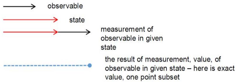 Fig. 1.1: States, observables, measurements on straight line In this classical kinematic example, it does not formally matter do we consider evolution of "state" or of "measurement of observable by the state" or of "the result of measurement" because they differ only by an additive constant or the map of one-dimensional vector to its length. The above one-dimensional situation radically changes if the process entities become belonging to a plane, that's dimensionality of physical process increases, though we continue watching results in one dimensional projection (see Fig.1.2): 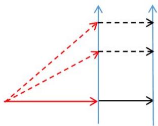 Fig. 1.2: States, observables, measurements on plane, projected on straight line infinitely many states (dash red) give the same measurement of observable in 1D In a not deterministic evolution, the central point of randomness of observed values is the fact that their probabilities are associated with partition of the space of states. Each partition element is fiber (level set)[^3] of each of the observable value under the action of the state on observable. Probabilities are (relative) measures of those fibers (see Fig.1.3): 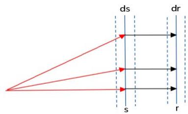 Fig. 1.3: Probabilities as measures of partition elements Probability to get result of measurement in interval dr around r (making no sense to say "find system in state r" as in conventional quantum mechanics) is the integral of probability density of states over the strip ds. The option to expand, to lift the space where physical processes are considered, may have critical consequence to a theory. A kind of expanding is the core of the suggested formulation aimed at the theory deeper than conventional quantum mechanics. ## II. WORKING WITH G-QUBITS INSTEAD OF QUBITS A theory that is an alternative to conventional quantum mechanics has been under development for a while, see, [1], [^2], [^4], [^5]. Its novel features are: - Replacing complex numbers by elements of even subalgebra of geometric algebra in three dimensions, that's by elements of the form "scalar plus bivector". - Elementary physical objects follow the structure: position in space plus explicitly defined object as the $G_{3}$, geometric algebra in three dimensions, elements. - Operators acting on those objects are identified as direct sums of position translation and points on the three-sphere $\mathbb{S}^3$ defining rotations. Those points are connected, due to hedgehog theorem, by parallel (Clifford) translations. - Evolution of the $\mathbb{S}^3$ part of operators by Clifford translations is governed by generalization of the Schrodinger equation with unit bivectors in three dimensions instead of formal imaginary unit. In the following the $\mathbb{S}^3$ part of the operators will only be considered. Qubits, identifying states in conventional quantum mechanics, mathematically are elements of the two-dimensional complex spaces: $\binom{x_1+iy_1}{x_2+iy_2}$, conditioned by $\| x_1 + iy_1\|^2 + \| x_2 + iy_2\|^2 = 1$, that is unit value elements of $C^2$. Imaginary unit $i$ is used formally with the property $i^2 = -1$. In another accepted notations a qubit is: $$ C ^ {2} \ni {\binom {z _ {1}} {z _ {2}}} = z _ {1} {\binom {1} {0}} + z _ {2} {\binom {0} {1}} = z _ {1} | 0 \rangle + z _ {2} | 1 \rangle $$ In the suggested formalism complex numbers $x + iy$ are replaced with elements of even subalgebra of $G_{3}$ - geometric algebra in three dimensions. Even subalgebra $G_3^+$ is subalgebra of elements of the form $M_3 = \alpha + I_S\beta$, where $\alpha$ and $\beta$ are (real) scalars and $I_S$ is some unit bivector arbitrary placed in three-dimensional space. Elements of $G_3^+$ can be depicted as in Fig. 2.1. 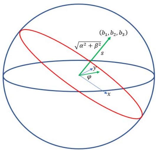 Fig. 2.1: An element of $G_3^+$ Unit value elements of $G_3^+$, when $\alpha^2 + \beta^2 = 1$, will be called g-qubits. The wave functions (states in the suggested approach) implemented as g-qubits store much more information than qubits, see Fig 2.2. 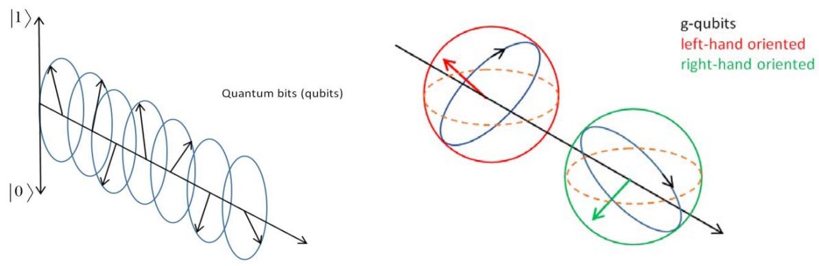 Fig. 2.2: Geometrically pictured qubits and g-qubits ## III. LIFT OF QUBITS TO G-QUBITS ### a) Lift of quantum mechanical qubit states to $g$ -qubits Take right-hand screw oriented basis $\{B_1, B_2, B_3\}$ of unit value bivectors, with the multiplication rules $B_1B_2 = -B_3$, $B_1B_3 = B_2$, $B_2B_3 = -B_1$, $I_3B_1I_3B_2I_3B_3 = I_3$ (or equivalently $B_1B_2B_3 = 1$ ), where $I_3$ is oriented unit value volume, pseudoscalar, in three dimensions, see Fig.3.1. 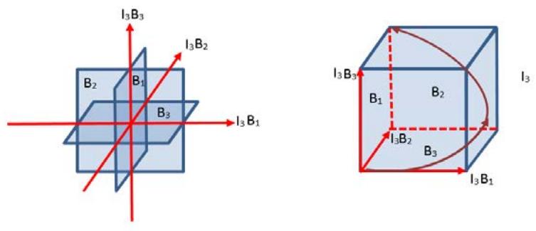 Fig. 3.1: Basis of bivectors, dual vectors and unit value pseudoscalar The quantum mechanical qubit state, $|\psi \rangle = z_1|0\rangle + z_2|1\rangle$, is linear combination of two basis states $|0\rangle$ and $|1\rangle$. In the $G_{3}^{+}$ terms these two states correspond to the following classes of equivalence in $G_{3}^{+}$, depending particularly on which basis bivector is selected as complex plane: - If $B_{1}$ is taken as complex plane, then - State $|0\rangle$ has fiber (level set) of the $G_3^+$ elements $so(\alpha, \beta, S)_{|0\rangle}$ (0-type $G_3^+$ states): $$ \alpha + \beta_1 B_1, \alpha^2 + \beta_1^2 = 1 $$ - State $\left| 1\right\rangle$ has fiber of the ${G}_{3}^{ + }$ elements so ${\left( \alpha,\beta,S\right) }_{\left| 1\right\rangle }$ (1-type ${G}_{3}^{ + }$ states): $$ \beta_ {3} B _ {3} + \beta_ {2} B _ {2} = (\beta_ {3} + \beta_ {2} B _ {1}) B _ {3}, \beta_ {3} ^ {2} + \beta_ {2} ^ {2} = 1 $$ - If $B_{1}$ is taken as complex plane, then - State $|0\rangle$ has fiber (level set) of the $G_{3}^{+}$ elements $so(\alpha, \beta, S)_{|0\rangle}$ (0-type $G_{3}^{+}$ states): $$ \alpha + \beta_ {2} B _ {2}, \alpha^ {2} + \beta_ {2} ^ {2} = 1 $$ - State $\left| 1\right\rangle$ has fiber of the ${G}_{3}^{ + }$ elements so ${\left( \alpha,\beta,S\right) }_{\left| 1\right\rangle }$ (1-type ${G}_{3}^{ + }$ states): $$ \beta_ {1} B _ {1} + \beta_ {3} B _ {3} = (\beta_ {1} + \beta_ {3} B _ {2}) B _ {1}, \beta_ {1} ^ {2} + \beta_ {3} ^ {2} = 1 $$ - If $B_{3}$ is taken as complex plane, then - State $|0\rangle$ has fiber (level set) of the $G_3^+$ elements so $(\alpha, \beta, S)_{|0\rangle}$ (0-type $G_3^+$ states): $$ \alpha + \beta_ {3} B _ {3}, \alpha^ {2} + \beta_ {3} ^ {2} = 1 $$ - State $\left| 1\right\rangle$ has fiber of the ${G}_{3}^{ + }$ elements so ${\left( \alpha,\beta,S\right) }_{\left| 1\right\rangle }\left( {1 - \text{type }{G}_{3}^{ + }\text{states}}\right)$: $$ \beta_ {1} B _ {1} + \beta_ {2} B _ {2} = (\beta_ {2} + \beta_ {1} B _ {3}) B _ {2}, \beta_ {2} ^ {2} + \beta_ {1} ^ {2} = 1 $$ ### b) Implementation of definitions 1.1 in the $g$ -qubit state case General definition of measurement in the suggested approach is based on: - the set of observables, particularly elements of $G_3^+$, - the set of states, normalized elements of $G_3^+$, g-qubits, - special case of measurement of a $G_3^+$ observable $C = C_0 + C_1B_1 + C_2B_2 + C_3B_3$ by g-qubit (wave function) $\alpha + I_S\beta = \alpha + \beta_1B_1 + \beta_2B_2 + \beta_3B_3$ is defined as $$ (\alpha - I _ {S} \beta) C (\alpha + I _ {S} \beta) $$ with the result: $$ C _ {0} + C _ {1} B _ {1} + C _ {2} B _ {2} + C _ {3} B _ {3} \xrightarrow {\alpha + \beta_ {1} B _ {1} + \beta_ {2} B _ {2} + \beta_ {3} B _ {3}} C _ {0} + $$ $$ \left(C _ {1} \left[ \left(\alpha^ {2} + \beta_ {1} ^ {2}\right) - \left(\beta_ {2} ^ {2} + \beta_ {3} ^ {2}\right) \right] + 2 C _ {2} \left(\beta_ {1} \beta_ {2} - \alpha \beta_ {3}\right) + 2 C _ {3} \left(\alpha \beta_ {2} + \beta_ {1} \beta_ {3}\right)\right) B _ {1} + $$ $$ (2C_{1}(\alpha\beta_{3} + \beta_{1}\beta_{2}) + C_{2}[(\alpha^{2} + \beta_{2}^{2}) - (\beta_{1}^{2} + \beta_{3}^{2})] + 2C_{3}(\beta_{2}\beta_{3} - \alpha\beta_{1}))B_{2} + $$ $$ \left(2 C _ {1} \left(\beta_ {1} \beta_ {3} - \alpha \beta_ {2}\right) + 2 C _ {2} \left(\alpha \beta_ {1} + \beta_ {2} \beta_ {3}\right) + C _ {3} \left[ \left(\alpha^ {2} + \beta_ {3} ^ {2}\right) - \left(\beta_ {1} ^ {2} + \beta_ {2} ^ {2}\right) \right]\right) B _ {3} \tag{3.1} $$ Since g-qubit (state, wave function) is normalized, the measurement can be written in exponential form: $$ e ^ {- I s \varphi} C e ^ {I s \varphi} $$ where $\varphi = \cos^{-1}\alpha$ The lift from $C^2$ to $G_3^+$ needs a $\{B_1, B_2, B_3\}$ reference frame of unit value bivectors. This frame, as a solid, can be arbitrary rotated in three dimensions. In that sense we have principal fiber bundle $G_3^+ \to C^2$ with the standard fiber as group of rotations which is also effectively identified by elements of $G_3^+$. Suppose we are interested in the probability of the result of measurement in which the observable component $C_1B_1$ does not change. This is relative measure of states $\sqrt{\alpha^2 + \beta_1^2}\left(\frac{\alpha}{\sqrt{\alpha^2 + \beta_1^2}} +\frac{\beta_1}{\sqrt{\alpha^2 + \beta_1^2}} B_1\right)$ in the measurements: $$ \sqrt{\alpha^2 + \beta_1^2} \left( \frac{\alpha}{\sqrt{\alpha^2 + \beta_1^2}} - \frac{\beta_1}{\sqrt{\alpha^2 + \beta_1^2}} B_1 \right) C \sqrt{\alpha^2 + \beta_1^2} \left( \frac{\alpha}{\sqrt{\alpha^2 + \beta_1^2}} + \frac{\beta_1}{\sqrt{\alpha^2 + \beta_1^2}} B_1 \right) $$ That measure is equal to $\alpha^2 + \beta_1^2$, that is equal to $z_1^2$ in the down mapping from $G_3^+$ to $z_1|0\rangle + z_2|1\rangle$. Thus, we have clear explanation of common quantum mechanics wisdom on "probability of finding system in state $|0\rangle$ ". Similar calculations explain correspondence of $\beta_3^2 +\beta_2^2$ to $z_{2}^{2}$ in the qubit $z_{1}|0\rangle +$ $z_{2}1\rangle$ when the component $C_1B_1$ in measurement just got flipped. Any arbitrary $G_3^+$ state $so(\alpha, \beta, S) = \alpha + \beta_1 B_1 + \beta_2 B_2 + \beta_3 B_3$ can be rewritten either as 0-type state or 1-type state: $$ \alpha + \beta_ {1} B _ {1} + \beta_ {2} B _ {2} + \beta_ {3} B _ {3} = \alpha + I _ {S (\beta_ {1}, \beta_ {2}, \beta_ {3})} \sqrt {\beta_ {1} ^ {2} + \beta_ {2} ^ {2} + \beta_ {3} ^ {2}}, $$ where $I_{S(\beta_1,\beta_2,\beta_3)} = \frac{\beta_1B_1 + \beta_2B_2 + \beta_3B_3}{\sqrt{\beta_1^2 + \beta_2^2 + \beta_3^2}}$ 0-type, or $$ \alpha + \beta_ {1} B _ {1} + \beta_ {2} B _ {2} + \beta_ {3} B _ {3} = (\beta_ {3} + \beta_ {2} B _ {1} - \beta_ {1} B _ {2} - \alpha B _ {3}) B _ {3} = (\beta_ {3} + \beta_ {2} B _ {1} - \beta_ {1} B _ {2}) B _ {3}. $$ $$ I _ {S (\beta_ {2}, - \beta_ {1}, - \alpha)} \sqrt {\alpha^ {2} + \beta_ {1} ^ {2} + \beta_ {2} ^ {2}}) B _ {3}, $$ where $I_{S(\beta_2, - \beta_1, - \alpha)} = \frac{\beta_2B_1 - \beta_1B_2 - \alpha B_3}{\sqrt{\alpha^2 + \beta_1^2 + \beta_2^2}}$ 1-type. All that means that any $G_3^+$ state $\alpha + \beta_1 B_1 + \beta_2 B_2 + \beta_3 B_3$ measuring observable $C_1 B_1 + C_2 B_2 + C_3 B_3$ does not change the observable projection onto plane of $I_{S(\beta_1, \beta_2, \beta_3)} = \frac{\beta_1 B_1 + \beta_2 B_2 + \beta_3 B_3}{\sqrt{\beta_1^2 + \beta_2^2 + \beta_3^2}}$ and just flips the observable projection onto plane $I_{S(\beta_2, -\beta_1, -\alpha)} = \frac{\beta_2 B_1 - \beta_1 B_2 - \alpha B_3}{\sqrt{\alpha^2 + \beta_1^2 + \beta_2^2}}$. ## IV. EVOLUTION OF G-QUBIT STATES Measurement of observable $C$ by a state $e^{I_S\varphi}$ is defined as $e^{-I_S\varphi}Ce^{I_S\varphi}$. Evolution of a state is its movement on surface of $\mathbb{S}^3$. Consider necessary formalism. Multiplication of two geometric algebra exponents reads, see Sec.1.2 of \[^5\]: $$ \begin{array}{l} e ^ {I _ {S _ {1}} \alpha} e ^ {I _ {S _ {2}} \beta} = \left(\cos \alpha + I _ {S _ {1}} \sin \alpha\right) \left(\cos \beta + I _ {S _ {2}} \sin \beta\right) \\= \cos \alpha \cos \beta + I _ {S _ {1}} \sin \alpha \cos \beta + I _ {S _ {2}} \cos \alpha \sin \beta + I _ {S _ {1}} I _ {S _ {2}} \sin \alpha \sin \beta \\\end{array} $$ It follows from the formula for bivector multiplication: $$ g _ {1} g _ {2} = \alpha_ {1} \alpha_ {2} - (s _ {1} \cdot s _ {2}) \beta_ {1} \beta_ {2} + I _ {S _ {1}} \alpha_ {2} \beta_ {1} + I _ {S _ {2}} \alpha_ {1} \beta_ {2} - I _ {3} (s _ {1} \times s _ {2}) \beta_ {1} \beta_ {2} $$ with vectors to which the unit bivectors $I_{S_1}$ and $I_{S_2}$ are duals: $s_1 = -I_3I_{S_1}$, $s_2 = -I_3I_{S_2}$. In the current case $$ \alpha_ {1} = \cos \alpha , \alpha_ {2} = \cos \beta , \beta_ {1} = \sin \alpha , \beta_ {2} = \sin \beta , $$ and we get above formula for $e^{I_{S_1}\alpha}e^{I_{S_2}\beta}$ The product of two exponents is again an exponent, because generally $|g_1 g_2| = |g_1||g_2|$ and $\left|e^{I_{S_1} \alpha} e^{I_{S_2} \beta}\right| = \left|e^{I_{S_1} \alpha}\right| \left|e^{I_{S_2} \beta}\right| = 1$, see Sec.1.3 of [^5]. Multiplication of an exponent by another exponent is often called Clifford translation. Using the term translation follows from the fact that Clifford translation does not change distances between the exponents it acts upon when we identify exponents as points on unit sphere $\mathbb{S}^3$: $$ \begin{array}{l} \cos \alpha + I _ {S} \sin \alpha = \cos \alpha + b _ {1} \sin \alpha B _ {1} + b _ {2} \sin \alpha B _ {2} + b _ {3} \sin \alpha B _ {3} \\\Leftrightarrow \{\cos \alpha , b _ {1} \sin \alpha , b _ {2} \sin \alpha , b _ {3} \sin \alpha \} \\\end{array} $$ $$ (\cos \alpha) ^ {2} + (b _ {1} \sin \alpha) ^ {2} + (b _ {2} \sin \alpha) ^ {2} + (b _ {3} \sin \alpha) ^ {2} = 1 $$ This result follows again from $|g_1 g_2| = |g_1||g_2|$: $$ \left| e ^ {I _ {S} \alpha} (g _ {1} - g _ {2}) \right| = \left| e ^ {I _ {S} \alpha} \right| \left| g _ {1} - g _ {2} \right| = \left| g _ {1} - g _ {2} \right| $$ Assume the angle $\alpha$ in Clifford translation is a variable one. Then in the case $I_{S_1} =$ const: $$ \frac {\partial}{\partial \alpha} e ^ {I _ {S _ {1}} \alpha} = I _ {S _ {1}} e ^ {I _ {S _ {1}} \alpha} $$ If $I_{S_1}$ is dual to some unit vector $H$, $I_{S_1} = -I_3H$ (this is the case of the matrix Hamiltonian map to $G_3^+$, see [^3]), then $e^{I_{S_1}\alpha} = e^{-I_3H\alpha} \equiv \psi(H, \alpha)$ and $$ \frac {\partial}{\partial \alpha} \psi (H, \alpha) = - I _ {3} H \psi (H, \alpha) $$ that is obviously Geometric Algebra generalization of the Schrodinger equation. If vector $H$ varies in time we get, assuming $\alpha \equiv t$: $$ \frac{\partial}{\partial t} \psi (H (t), t) = I _ {3} \left(- H (t) - t \frac{\partial}{\partial t} H ( t )\right) \psi (H (t), t) $$ with, generally, $\psi (H(t),t) = e^{-I_3\left(\frac{H(t)}{|H(t)|}\right)|H(t)|t}$. Assume again constant $H$ and its unit length, $|H| = 1$. We see that displacement with $\alpha = \Delta t$ along big circle, intersection of the unit sphere $\mathbb{S}^3$ by plane $-I_3H$, rotates $\psi(H,t)$ lying on $\mathbb{S}^3$ by angle $\Delta t$ in that plane. Let us take two planes orthogonal to the plane of $-I_3H$ and comprising right-hand screw with it: $-I_3H_1$ and $-I_3H_2$. Right-handedness means: $$ (-I_3H)(-I_3H_1)=I_3H_2 $$ $$ \left(- I _ {3} H\right) \left(- I _ {3} H _ {2}\right) = - I _ {3} H _ {1} and $$ $$ (-I_3H_1)(-I_3H_2) = -I_3H $$ (See the earlier definition of the right-hand oriented triple of basis bivectors.) Then the three above formulas mean that the planes $-I_3H_1$ and $-I_3H_2$ rotate synchronically with $-I_3H$, correspondingly in planes $-I_3H_2$ and $-I_3H_1$. Thus, the triple of planes ro tates as solid while moving along big circle on $\mathbb{S}^3$. ## V. DOUBLE-SLIT EXPERIMENT Taking the set of g-qubits and projection of them onto $C^2$: $\pi \colon G_3^+ \to C^2$, we get fiber bundle. The projection depends on which basis bivector plane is selected as corresponding to formal imaginary unit plane. If we take, for example $B_3$, the projection is: $$ \pi \colon s o (\alpha , \beta , S) = \alpha + \beta_ {1} B _ {1} + \beta_ {2} B _ {2} + \beta_ {3} B _ {3} \to \left( \begin{array}{c} \alpha + i \beta_ {3} \\\beta_ {2} + i \beta_ {1} \end{array} \right) $$ Then for any $z = \begin{pmatrix} x_1 + iy_1 \\ x_2 + iy_2 \end{pmatrix} \in C^2$ the fiber in $G_3^+$ consists of all elements $F_z = x_1 + y_2B_1 + x_2B_2 + y_1B_3$ with an arbitrary triple of orthonormal bivectors $\{B_1, B_2, B_3\}$ satisfying multiplication rules. That particularly means that the standard fiber is a group of rotations of basis bivectors in the standard fiber $F_z$. Thus, the fiber bundle is principal fiber bundle. Let one first slit is only open, and the fiber, wave function, is some $F^1 = x_1^1 + y_2^1 B_1 + x_2^1 B_2 + y_1^1 B_3$. For the only open second slit the fiber is different: $F^2 = x_1^2 + y_2^2 B_1 + x_2^2 B_2 + y_1^2 B_3$. When both slits are open the corresponding fiber is defined by connection, parallel transport anywhere between fibers $F^1$ and $F^2$. Let we have a smooth curve $\gamma(t, P_1, P_2), 0 \leq t \leq 1$, connecting points $P_1 = (x_1^1, y_2^1, x_2^1, y_1^1)$ and $P_2 = (x_1^2, y_2^2, x_2^2, y_1^2)$, on three-dimensional sphere $\mathbb{S}^3$ such that $\gamma(0, P_1, P_2) = P_1$ and $\gamma(1, P_1, P_2) = P_2$. The easiest way to define parallel transport is $\gamma(t, P_1, P_2) = (1 - t)P_1 + tP_2$. For convenience purposes let us write $F^1$ and $F^2$ as exponents: $$ F^{1} = x_{1}^{1} + y_{2}^{1} B_{1} + x_{2}^{1} B_{2} + y_{1}^{1} B_{3} = x_{1}^{1} + \sqrt{(y_{2}^{1})^{2} + (x_{2}^{1})^{2} + (y_{1}^{1})^{2}} \left(\frac{y_{2}^{1}}{\sqrt{(y_{2}^{1})^{2} + (x_{2}^{1})^{2} + (y_{1}^{1})^{2}}} B_{1} + \frac{x_{2}^{1}}{\sqrt{(y_{2}^{1})^{2} + (x_{2}^{1})^{2} + (y_{1}^{1})^{2}}} B_{2} + \frac{y_{1}^{1}}{\sqrt{(y_{2}^{1})^{2} + (x_{2}^{1})^{2} + (y_{1}^{1})^{2}}} B_{3}\right) = e^{I_{S_{1}} \varphi_{1}}, $$ where $\varphi_{1} = \cos^{-1}x_{1}^{1}$ $$ I_{S_{1}} = \frac{y_{2}^{1}}{\sqrt{(y_{2}^{1})^{2} + (x_{2}^{1})^{2} + (y_{1}^{1})^{2}}} B_{1} + \frac{x_{2}^{1}}{\sqrt{(y_{2}^{1})^{2} + (x_{2}^{1})^{2} + (y_{1}^{1})^{2}}} B_{2} + \frac{y_{1}^{1}}{\sqrt{(y_{2}^{1})^{2} + (x_{2}^{1})^{2} + (y_{1}^{1})^{2}}} B_{3}. $$ Angle $\varphi_{1}$ is not uniquely defined since it can be any of $\cos^{-1}x_1^1\pm 2\pi k_1,k_1 = 0,1,2,\ldots$ where $\cos^{-1}x_1^1$ is, by definition, taken from interval $[0,\pi ]$. The angle $\cos^{-1}x_1^1$ will be denoted as $\varphi_{1}(0)$. $$ F^{2} = x_{1}^{2} + y_{2}^{2} B_{1} + x_{2}^{2} B_{2} + y_{1}^{2} B_{3} = x_{1}^{2} + \sqrt{(y_{2}^{2})^{2} + (x_{2}^{2})^{2} + (y_{1}^{2})^{2}} \left(\frac{y_{2}^{2}}{\sqrt{(y_{2}^{2})^{2} + (x_{2}^{2})^{2} + (y_{1}^{2})^{2}}} B_{1} + \frac{x_{2}^{2}}{\sqrt{(y_{2}^{2})^{2} + (x_{2}^{2})^{2} + (y_{1}^{2})^{2}}} B_{2} + \frac{y_{1}^{2}}{\sqrt{(y_{2}^{2})^{2} + (x_{2}^{2})^{2} + (y_{1}^{2})^{2}}} B_{3}\right) = e^{I S_{2} \varphi_{2}}, $$ where $\varphi_{2} = \cos^{-1}x_{1}^{2}$ $$ I _ {S _ {2}} = \frac {y _ {2} ^ {2}}{\sqrt {\left(y _ {2} ^ {2}\right) ^ {2} + \left(x _ {2} ^ {2}\right) ^ {2} + \left(y _ {1} ^ {2}\right) ^ {2}}} B _ {1} + \frac {x _ {2} ^ {2}}{\sqrt {\left(y _ {2} ^ {2}\right) ^ {2} + \left(x _ {2} ^ {2}\right) ^ {2} + \left(y _ {1} ^ {2}\right) ^ {2}}} B _ {2} + \frac {y _ {1} ^ {2}}{\sqrt {\left(y _ {2} ^ {2}\right) ^ {2} + \left(x _ {2} ^ {2}\right) ^ {2} + \left(y _ {1} ^ {2}\right) ^ {2}}} B _ {3}. $$ As above, $\varphi_{2} = \cos^{-1}x_{1}^{2}\pm 2\pi k_{2},k_{2} = 0,1,2,\ldots$ The angle $\cos^{-1}x_1^2$ will be denoted as $\varphi_{2}(0)$ Measurement of an observable $$ \begin{array}{l} C = C _ {0} + C _ {1} B _ {1} + C _ {2} B _ {2} + C _ {3} B _ {3} = C | \left(\frac{C _ {0}}{| C |} + \frac{C _ {1}}{| C |} B _ {1} + \frac{C _ {2}}{| C |} B _ {2} + \frac{C _ {3}}{| C |} B _ {3}\right) = \\| C | \left(\frac{C _ {0}}{| C |} + \sqrt{1 - \frac{C _ {0} ^ {2}}{| C | ^ {2}}} \left(\frac{C _ {1}}{| C | \sqrt{1 - \frac{C _ {0} ^ {2}}{| C | ^ {2}}}} B _ {1} + \frac{C _ {2}}{| C | \sqrt{1 - \frac{C _ {0} ^ {2}}{| C | ^ {2}}}} B _ {2} + \frac{C _ {3}}{| C | \sqrt{1 - \frac{C _ {0} ^ {2}}{| C | ^ {2}}}} B _ {3}\right)\right) = C | e ^ {I s \varphi}, \\\end{array} $$ $$ \begin{array}{l} \text{where} | C | = \sqrt{C _ {0} ^ {2} + C _ {1} ^ {2} + C _ {2} ^ {2} + C _ {3} ^ {2}}, \varphi = \cos^ {- 1} \frac{C _ {0}}{| C |}, I _ {S} = \frac{C _ {1}}{| C | \sqrt{1 - \frac{C _ {0} ^ {2}}{| C | ^ {2}}}} B _ {1} + \frac{C _ {2}}{| C | \sqrt{1 - \frac{C _ {0} ^ {2}}{| C | ^ {2}}}} B _ {2} + \\\frac{C _ {3}}{| C | \sqrt{1 - \frac{C _ {0} ^ {2}}{| C | ^ {2}}}} B _ {3}, \\\end{array} $$ by the wave function $e^{I S_{1}\varphi_{1}}$ is: $$ M_{1} = e^{-I_{S_{1}}\varphi_{1}} |C| e^{I_{S}\varphi} e^{I_{S_{1}}\varphi_{1}} $$ Measurement by $e^{I S_{2}\varphi_{2}}$ is: $$ M _ {2} = e ^ {- I _ {S _ {2}} \varphi_ {2}} | C | e ^ {I _ {S} \varphi} e ^ {I _ {S _ {2}} \varphi_ {2}} $$ Measurement by any intermediate parallel transport wave function $(1 - t)e^{I S_{1}\varphi_{1}} + te^{I S_{2}\varphi_{2}}$ then reads: $$ (1 - t)^{2} e^{-I S_{1} \varphi_{1}} |C| e^{I S \varphi} e^{I S_{1} \varphi_{1}} + t^{2} e^{-I S_{2} \varphi_{2}} |C| e^{I S \varphi} e^{I S_{2} \varphi_{2}} + $$ $$ |C|t(1-t)(e^{-I_{S_1}\varphi_1}e^{I_{S}\varphi}e^{I_{S_2}\varphi_2} + e^{-I_{S_2}\varphi_2}e^{I_{S}\varphi}e^{I_{S_1}\varphi_1}) = (1-t)^2e^{-I_{S_1}\varphi_1}|C|e^{I_{S}\varphi}e^{I_{S_1}\varphi_1} + t^2e^{-I_{S_2}\varphi_2}|C|e^{I_{S}\varphi}e^{I_{S_2}\varphi_2} + t(1-t)(e^{-I_{S_2}\varphi_2}e^{I_{S_1}\varphi_1}|C|e^{I_{S}\varphi}e^{I_{S_1}\varphi_1} + e^{-I_{S_1}\varphi_1}e^{I_{S_2}\varphi_2}|C|e^{I_{S}\varphi}e^{I_{S_2}\varphi_2}) $$ $$ t(1-t)(e^{-I_{S_1}\varphi_1}e^{I_{S_2}\varphi_2}e^{-I_{S_2}\varphi_2}|C|e^{I_{S}\varphi}e^{I_{S_2}\varphi_2} + e^{-I_{S_2}\varphi_2}e^{I_{S_1}\varphi_1}e^{-I_{S_1}\varphi_1}|C|e^{I_{S}\varphi}e^{I_{S_1}\varphi_1}) = (1-t)^2M_1 + t^2M_2 + t(1-t)(e^{-I_{S_2}\varphi_2}e^{I_{S_1}\varphi_1}M_1 + e^{-I_{S_1}\varphi_1}e^{I_{S_2}\varphi_2}M_2) $$ Let us make natural for double slit experiment assumption $S_{1} = S_{2} = S_{0}$ (that is the two wave functions, measuring states, are of 0-type with identical bivector planes.) Then we get the measurement result by the intermediate parallel transport wave function: $$ \begin{array}{l} (1 - t) ^ {2} M _ {1} + t ^ {2} M _ {2} + t (1 - t) \big (e ^ {- I _ {S _ {2}} \varphi_ {2}} e ^ {I _ {S _ {1}} \varphi_ {1}} M _ {1} + e ^ {- I _ {S _ {1}} \varphi_ {1}} e ^ {I _ {S _ {2}} \varphi_ {2}} M _ {2} \big) = \\(1 - t) ^ {2} M _ {1} + t ^ {2} M _ {2} + t (1 - t) \big (e ^ {I _ {S _ {0}} (\varphi_ {1} - \varphi_ {2})} M _ {1} + e ^ {I _ {S _ {0}} (\varphi_ {2} - \varphi_ {1})} M _ {2} \big) \\\end{array} $$ It is easily seen that the result of measurement is $M_{1}$ when $t = 0$ and $M_{2}$ when $t = 1$. Consider the following simplified scenario. Assume we are only interested in the projections of $M_1$ and $M_2$ onto the plane of their rotations, $S_0$, $M_1(S_0)$ and $M_2(S_0)$. Then from the general formula $$ e^{I_{S_2}\varphi_2} e^{I_{S_1}\varphi_1} = \cos\varphi_1\cos\varphi_2 - (s_1\cdot s_2)\sin\varphi_1\sin\varphi_2 + I_3 s_2\cos\varphi_1\sin\varphi_2 + I_3 s_1\cos\varphi_2\sin\varphi_1 - I_3 (s_2\times s_1)\sin\varphi_1\sin\varphi_2 $$ we get that up to some factors $e^{I_{S_0}(\varphi_1 - \varphi_2)}M_1(S_0)$ is $M_1(S_0)$ rotated in $S_0$ by angle $\varphi_1 - \varphi_2$ and $e^{I_{S_0}(\varphi_2 - \varphi_1)}M_2(S_0)$ is $M_2(S_0)$ rotated in $S_0$ by angle $\varphi_2 - \varphi_1$. Without loss of generality suppose that the angles $\varphi_{1}(0)$ and $\varphi_{2}(0)$ are equal by values but opposite in sign: $$ \varphi_ {1} (0) = - \varphi_ {0}, \varphi_ {2} (0) = \varphi_ {0}, $$ $$ \varphi_ {1} (0) - \varphi_ {2} (0) = - 2 \varphi_ {0} $$ $$ \varphi_ {2} (0) - \varphi_ {1} (0) = 2 \varphi_ {0} $$ Then it follows that in Clifford translations the projection $M_1(S_0)$ rotates in $S_0$ additionally by $-2\big(\varphi_0 \pm \pi(k_1 - k_2)\big), k_1 = 0,1,2,\ldots, k_2 = 0,1,2,\ldots$, and projection $M_2(S_0)$ rotates in $S_0$ additionally by $2\big(\varphi_0 \pm \pi(k_1 - k_2)\big), k_1 = 0,1,2,\ldots, k_2 = 0,1,2,\ldots$. Thus, in addition to $(1 - t)^2 M_1(S_0)$ and $t^2 M_2(S_0)$, we get infinite number of copies of $M_1(S_0)$ and $M_2(S_0)$ multiplied every time by $t(1 - t)$ and separated by $\pm 2\pi$ along the big circle of intersection of plane $S_0$ with the sphere $\mathbb{S}^3$, see Fig. 5.1. 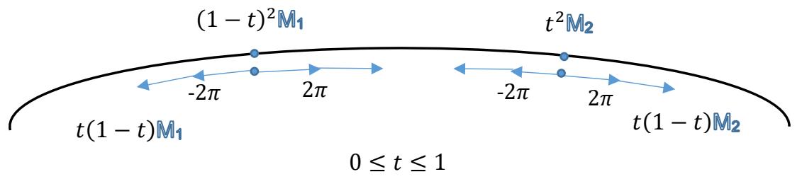 Fig. 5.1: Multiple results of measurements when both slits get opened ## VI. MODEL OF HYDROGEN ATOM Let the state has the Hamiltonian type form: $$ \psi (H (t), t) = e ^ {- I _ {3} \left(\frac {H (t)}{| H (t) |}\right) | H (t) | t} \tag {6.1} $$ where $H(t)$ is vector in three dimensions. An observable it will act upon is something of a torsion kind, $|r|e^{I_s\omega t}$. Thus, at instant of time $t$ we have the following result of action of state (6.1): $$ e ^ {I _ {3} \left(\frac{H (t)}{| H (t) |}\right) | H (t) | t} | r | e ^ {I _ {S} \omega t} e ^ {- I _ {3} \left(\frac{H (t)}{| H (t) |}\right) | H (t) | t} \tag{6.2} $$ The Hamiltonian type wave function (6.1) bears its origin from proton, while the observable $|r|e^{Is\omega t}$ represents electron. The geometric algebra existence of the hydrogen atom can only follow from stable sequence of measurement results (6.2) with appropriate combination(s) of $H(t)$ and $\omega$. Let $$ H (t) = - h _ {1} (t) I _ {3} B _ {1} - h _ {2} (t) I _ {3} B _ {2} - h _ {3} (t) I _ {3} B _ {3} $$ Then $|H(t)| = \sqrt{h_1^2(t) + h_2^2(t) + h_3^2(t)}$, bivector part of (6.1) is $\frac{\sin(|H(t)|t)}{|H(t)|} (h_1(t)B_1 + h_2(t)B_2 + h_3(t)B_3)$ and the scalar part of the wave function (6.1) is $\cos(|H(t)|t)$. If initial bivector plane of observable is$c_{1}B_{1} + c_{2}B_{2} + c_{3}B_{3}$,$c_{1}^{2} + c_{2}^{2} + c_{3}^{2} = 1$, scalar part then is$|r|\cos \omega t$, thus$|r|e^{I_S\omega t} = |r|\cos \omega t + |r|\sin \omega t(c_1(t)B_1 + c_2(t)B_2 + c_3(t)B_3)$. EXPLAINING SOME WEIRD QUANTUM MECHANICAL FEATURES IN GEOMETRIC ALGEBRA FORMALISM Let us denote the plane $-I_3\left(\frac{H(t)}{|H(t)|}\right) \equiv I_H$. Then the sequence of transformations (6.2) reads: $$ e^{-I_H|H|\Delta t} \Big( \dots \Big( e^{-I_H|H|\Delta t} \Big( e^{-I_H|H|t} |r| e^{I_S\omega t} e^{I_H|H|t} \Big) e^{I_H|H|\Delta t} \Big) \dots \Big) e^{I_H|H|\Delta t} $$ If $I_{S} = I_{H}$ and assuming that $H(t)$ does not depend on time, we get: $$ | r | e ^ {- I _ {H} | H | t} e ^ {I _ {H} \omega t} e ^ {I _ {H} | H | t} $$ Angular velocity $\omega$ should be synchronized with Hamiltonian rotation by $2|H|^5$, though it can be integer times greater than $2|H|$. Now assume that $I_S \neq I_H$. Thus, the result of (6.2) is: $$ \left| r \right| e ^ {- I _ {H} | H | t} e ^ {I _ {S} \omega t} e ^ {I _ {H} | H | t} $$ The vector of length $|r|$ rotates in plane $I_{S}$ with angular velocity $\omega$ while element $|r|e^{I_S\omega t}$ rotates in plane $I_{H}$. Again, for stability, angular velocity $\omega$ should be integer times greater than $2|H|$. Take the general formula (3.1) and substitute $C_0 = |r| \cos \omega t$, $C_1 = |r| c_1 \sin \omega t$, $C_2 = |r| c_2 \sin \omega t$, $C_3 = |r| c_3 \sin \omega t$, where $c_i$ are components of $I_S$ in the basis $\{B_1, B_2, B_3\}$, and $\alpha = \cos(|H|t)$, $\beta_i = h_i \sin(|H|t)$, $h_i$ are components of $I_H$ in the basis $\{B_1, B_2, B_3\}$: $I_H = h_1 B_1 + h_2 B_2 + h_3 B_3$. The result of measurement after multiple transformations reads: $$ \frac {| r | \sin 2 | H | t}{2 | H | ^ {2}} \bigg \{\big [ c _ {1} \big ((1 + \cos 2 | H | t) | H | ^ {2} + (1 - \cos 2 | H | t) (2 h _ {1} ^ {2} - | H | ^ {2}) \big) + \big [ c _ {2} \big ((1 + \cos 2 | H | t) | H | ^ {2} + (1 - \cos 2 | H | t) (2 h _ {2} ^ {2} - | H | ^ {2}) \big] \bigg \} $$ $$ 2 c _ {2} \left((1 - \cos 2 | H | t) h _ {1} h _ {2} - | H | h _ {3} \sin 2 | H | t\right) + 2 c _ {3} \big ((1 - \cos 2 | H | t) h _ {1} h _ {3} + $$ $$ \left. \left| H \right| \sin 2 | H | t h _ {2}) \right] B _ {1} + \left[ 2 c _ {1} \big ((1 - \cos 2 | H | t) h _ {1} h _ {2} - | H | h _ {3} \sin 2 | H | t \big) + \right. $$ $$ c _ {2} \left((1 + c o s 2 | H | t) | H | ^ {2} + (1 - c o s 2 | H | t) (2 h _ {2} ^ {2} - | H | ^ {2})\right) + 2 c _ {3} \left((1 - c o s 2 | H | t) h _ {2} h _ {3} - (1 - c o s 2 | H | t) h _ {1} h _ {3}\right) = 0. $$ $$ \left. \left| H \right| \sin 2 | H | t h _ {1}\right) \bigg ] B _ {2} + \left[ 2 c _ {1} \big ((1 - \cos 2 | H | t) h _ {1} h _ {3} - | H | \sin 2 | H | t h _ {2} \big) + 2 c _ {2} \big ((1 - \cos 2 | H | t) h _ {1} h _ {3} - | H | \sin 2 | H | t h _ {2} \big) \right] $$ $$ \begin{array}{l} \cos 2 | H | t) h _ {2} h _ {3} - | H | \sin 2 | H | t h _ {1}) + c _ {3} \big ((1 + \cos 2 | H | t) | H | ^ {2} + (1 - \cos 2 | H | t) (2 h _ {3} ^ {2} - \\| H | ^ {2})) \big) B _ {3} \end{array} \tag {6.3} $$ Formula (6.3) gives stable rotation of observable $|r| \cos \omega t + |r| \sin \omega t (c_1(t)B_1 + c_2(t)B_2 + c_3(t)B_3)$ (electron) due to action of the state $\psi(H(t),t) = e^{-I_3\left(\frac{H(t)}{|H(t)|}\right)|H(t)|t}$ (proton.) ## VII. CONCLUSIONS It was demonstrated that the geometric algebra formalism along with generalization of complex numbers and subsequent lift of the two-dimensional Hilbert space valued qubits to geometrically feasible elements of even subalgebra of geometric algebra in three dimensions allows, particularly, to resolve the double-slit experiment results with diffraction patterns inherent to wave diffraction. This weirdness of the double - slit experiment is milestone of all further difficulties in interpretation of conventional quantum mechanics. The approach also allows elimination of the Bohr's planetary model of the hydrogen atom. [^2]: One should say "by a state". State is operator acting on observable. _(p.2)_ [^3]: Recall that fiber of a point $y$ in $Y$ under a function $f: X \to Y$ is the inverse image of $\{y\}$ under $f: f^{-1}(\{y\}) = \{x \in X: f(x) = y\}$. _(p.3)_ [^4]: In the current formalism scalars can only be real numbers. "Complex" scalars make no sense anymore, see, for example, [2], [5]. _(p.4)_ [^5]: Rotation by the double of the exponential is known from rotational rules in three-dimensional geometric algebra, see, for example [3]. _(p.13)_

Generating HTML Viewer...

References

5 Cites in Article
Soiguine (2014). What quantum "state" really is?.
Alexander Soiguine (2015). The Geometric Algebra Lift of Qubits and Beyond.
Alexander Soiguine (2015). Explaining Some Weird Quantum Mechanical Features in Geometric Algebra Formalism.
Alexander Soiguine (1996). Complex Conjugation — Relative to What?.
Alexander Soiguine (2020). The Geometric Algebra Lift of Qubits and Beyond.
No ethics committee approval was required for this article type.
Data Availability
Not applicable for this article.
How to Cite This Article
Alexander Soiguine. 2026. \u201cExplaining Some Weird Quantum Mechanical Features in Geometric Algebra Formalism\u201d. Global Journal of Science Frontier Research - F: Mathematics & Decision GJSFR-F Volume 22 (GJSFR Volume 22 Issue F3).
Explore published articles in an immersive Augmented Reality environment. Our platform converts research papers into interactive 3D books, allowing readers to view and interact with content using AR and VR compatible devices.
Your published article is automatically converted into a realistic 3D book. Flip through pages and read research papers in a more engaging and interactive format.
Our website is actively being updated, and changes may occur frequently. Please clear your browser cache if needed. For feedback or error reporting, please email [email protected]
Thank you for connecting with us. We will respond to you shortly.