This Paper investigates the behavior of daily exchange rates between USD/INR, GBP/INR, CHF/INR and JPY/INR. This Paper attempts to examine the performance of ARCH/GARCH model in forecasting the currencies traded in Indian foreign exchange markets. The accuracy of the forecast is compared with Mean Error (ME), Mean Absolute Error (MAE), Mean Percentage error (MPE), Mean Absolute Percentage Error (MAPE) and Root Mean Squared Error (RMSE), Mean Absolute Square Error. Study the performance indicators of model by using AIC and BIC values. This paper attempts to examine the performance of ARCH/GARCH model in forecasting the currencies traded in Indian foreign exchange markets. Study the Forecasting value of next 5 years exchange rates USD American dollar, GBP British Pound, CHF Swiss Franc and JPY Japanese JPY currencies with INR Indian data from that investigates the behavior of daily exchange rates between USD/INR, GBP/INR, CHF/INR and JPY/INR.
## I. INTRODUCTION
Generally, we use ARMA model for evaluate conditional mean and ARCH to evaluate Conditional variance or Volatility or Dispersion. We are more interested to find out conditional variance, because we want to use the past history to forecast the variance. In financial market depends on "Volatility is clustering" implies time varying conditional variance.
In financial marketing risk has become an important part both for risk management and for regulatory purposes. Different investors have different levels of risk that they willing to take volatility is perceived as a measure of risk.
ARMA models are mainly focused on to model the conditional expectation of a process given the past, but in an ARMA model the conditional variance given the past is constant. What does this mean for, say, modeling stock returns? Suppose we have noticed that recent daily returns have been unusually volatile. We might forecast that tomorrow's return is also more variable than usual. However, an ARMA model cannot capture this type of behavior because its conditional variance is constant. So we need improved time series models if we desire to model the non constant volatility. In this paper we look at ARCH and GARCH time series models that are becoming widely used in econometrics and finance because they have randomly varying volatility. ARCH is an acronym meaning Auto Regressive Conditional Heteroscedasticity. In ARCH models the conditional variance has a structure very similar to the structure of the conditional expectation in an AR model. We first study the ARCH (1) model, which is the simplest GARCH model and similar to an AR (1) model. Then we look at ARCH (p) models that are analogous to AR (p) models. Finally, we look at GARCH (Generalized ARCH) models that model conditional variances much as the conditional expectation is modeled by an ARMA model.
Econometricians are being asked to forecast and analyze the size of the errors of the model. In this case the questions are about volatility and the standard tools have become the ARCH/GARCH models. The basic version of the least squares model assumes that, the expected value of all error terms when squared is the same at any given point. This assumption is called homoskedasticity and it is this assumption that is the focus of ARCH/GARCH models.
ARCH models were introduced by Engle (1982) generalized autoregressive conditional heteroscedasticity (GARCH) (Bollerslev, 1986) were developed early in stock market forecasting. However, these models are generally not effective tools for forecasting due to the non-linearity of data and the occurrence of shocks (Sharma et al. 2016). The model assumes that the variance of the current error term is related to the size of previous period error terms.
Emerson Rodolfo Abraham et al (2020) study the Time Series Prediction with Artificial Neural Networks: An Analysis Using Brazilian Soybean Production. In this paper they were collected the data 1961-2016 regarding soybean production in Brazil. The results reveal that ANN is the best approach to predict soybean harvest area and production while classical linear function remains more effective to predict soybean yield.
The work of Babu et al (2014) proposed a hybrid system based on ARIMA and GARCH models. The authors collected data from January 2010 to January 2011 to define the first dataset (TD1) used for evaluating the performance of their model. As reported in this, they compared results between the proposed approach and other autoregressive models such as ARIMA, GARCH etc. The corresponding errors measures (MAPE, MAE, MaxAPE and RMSE) show that the proposed approach outperforms other models. Furthermore, the authors considered SBI shares from January 2010 to December 2010 to test the performance of proposed approach. The error performance measures (MAE, MaxAPE, etc.) confirmed that the proposed method obtains better results among others model (ARIMA and GARCH single scenario etc.). Also, the proposed hybrid system minimizes error performance. Despite achieving considerable results, autoregressive models present several limitations for stock price prediction compared to ML-based techniques.
Hamilton (1994) proposed the increasing interest in predicting the future behavior of complex systems by involving a temporal component. Researchers have investigated this problem modeling a convenient representation for financial data, the so-called time series (i.e., numerical data points observed sequentially through time). Previous studies have highlighted the difficulty studying financial time series accurately due to their non-linear and non-stationary patterns.
Dinesh et al (2021) studied the Integration of genetic algorithm with artificial neural network for stock market forecasting. In this they were proposed an intelligent forecasting method based on a hybrid of an Artificial Neural Network (ANN) and a
Genetic Algorithm (GA) and uses two US stock market indices, DOW30 and NASDAQ100, for forecasting. The data were partitioned into training, testing, and validation datasets. The model validation was done on the stock data of the COVID-19 period. The experimental findings obtained using the DOW30 and NASDAQ100 reveal that the accuracy of the GA and ANN hybrid model for the DOW30 and NASDAQ100 is greater than that of the single ANN (BPANN) technique, both in the short and long term.
Various ARCH models have been applied by researchers to analyze the volatility of exchange rates in different countries. For example some studies are: (Benavides, 2006) in which the author analyses the volatility forecast for the Mexican Peso – U.S. Dollar exchange rate, (Trenca et. al., 2011) which analyzes the evolution of the exchange rate for: Euro/RON, dollar/RON, yen/RON, British pound/RON, Swiss franc/RON for a period of five years from 2005 until 2011, (Alam et. al., 2012) in which the authors analyze exchange rates of Bangladeshi Taka (BDT) against the U.S. Dollar (USD) for the period of July 03, 2006 to April 30, 2012, (Musa et. al, 2014) forecast the exchange rate volatility between Naira and US Dollar using GARCH models.
## II. LITERATURE REVIEW
### a) Arch Model
ARCH is as AR component except we use lag or variance rather than lag of dependent variable.
The following reasons for the ARCH success:
- ARCH models are simple and easy to handle
- ARCH models take care of clustered errors
- ARCH models take care of nonlinearities
- ARCH models take care of changes in the econometrician's ability to forecast. The basic equation of estimation of parameters in ARCH model is given in (4.2.2)
Let $\mathbf{Y}_{\mathrm{t}}$ be $\mathbf{N}$ (0, 1). The process $\mathbf{Z}_{\mathrm{t}}$ is an ARCH (q) process if it is stationary and if it satisfies for all 't' and some strictly positive valued process $\sigma_{t}$, the equations
$$
Z_{t} = \sigma_{t} Y_{t}
$$
$$
\sigma_{t}^{2} = \varphi_{0} + \xi_{1} Y_{t-1}^{2} + \xi_{2} Y_{t-2}^{2} + \dots + \xi_{q} Y_{ t-q}^{2} \tag{2}
$$
Constraints on parameters:
variance has to be positive:
$$
\varphi_ {0} > 0, \xi_ {1}, \xi_ {2}, \ldots , \xi_ {q - 1} \geq 0, \xi_ {q} > 0
$$
Stationary:
$$
\xi_ {1} + \xi_ {2} + \dots + \xi_ {q} < 1
$$
### b) Garch Model
GARCH is as MA component except we use past error of variance equation rather than past error of mean equation. In ARCH model computational problems may arise when the polynomial presents a high order. To facilitate such computation, Bollerslev (1986) proposed a Generalized Autoregressive Conditional Heteroskedasticity
(GARCH) model. GARCH (p,q) model (generalized autoregressive conditional heteroskedasticity) - equation for variance $\sigma_t^2$.
$$
\sigma_t^2 = \varphi_0 + \xi_1 Y_{t-1}^2 + \xi_2 Y_{t-2}^2 + \ldots + \xi_q Y_{t-q}^2 + \delta_1 \sigma_{t-1}^2 + \delta_2 \sigma_{t-2}^2 + \ldots + \delta_q \sigma_{t-p}^2 \quad \ldots (3)
$$
It is quite obvious the similar structure of Autoregressive Moving Average (ARMA) and GARCH processes: a GARCH $(\mathfrak{p},\mathfrak{q})$ has a polynomial $\delta$ (L) of order "p" - the autoregressive term, and a polynomial $\xi$ (L) of order "q" - the moving average term.
### c) Estimation of Value at Risk (VAR)
Value at Risk (VaR) estimates the maximum expected loss on an investment, over a given period of time and given a specified degree of confidence. A value at risk statistic has three components: a time period, a confidence level and a loss amount (expressed either in currency or loss percentage). Value at risk answers question like what is the worst I can, with a $95\%$ or $99\%$ level of confidence, expect to lose in investment over the next day, month or year. According to Glyn (2014) value at risk is given by
$$
V a r = \mu + Z _ {\alpha} \sigma \tag {4}
$$
In this research, value at risk (VaR) will be estimated using GARCH models identified between USD/INR, GBP/INR, CHF/INR and JPY/INR on the foreign exchange rate.
### d) Methodology
ARCH and GARCH models have become important tools in the analysis of time series data, particularly in financial application. These models are especially useful when the goal of the study is to analyse and forecast volatility. This study investigates the volatility in foreign exchange rate.
This Paper investigates the behavior of daily exchange rates between USD/INR, GBP/INR, CHF/INR and JPY/INR. This Paper attempts to examine the performance of ARCH/GARCH model in forecasting the currencies traded in Indian foreign exchange markets. This paper attempts to examine the performance of ARCH/GARCH model in forecasting the currencies traded in Indian foreign exchange markets. Study the Forecasting value of next 5 years exchange rates USD American dollar, GBP British Pound, CHF Swiss Franc and JPY Japanese JPY currencies with INR Indian data from that investigates the behavior of daily exchange rates between USD/INR, GBP/INR, CHF/INR and JPY/INR.
Objectives: Constructing ARCH/GARCH model for the investigated time series includes the following flowchart:
### e) Check for Stationarity
Check for stationarity of daily exchange rates between USD/INR, GBP/INR, CHF/INR and JPY/INR data.
Forex GBP/INR ARIMA residuals
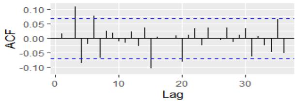
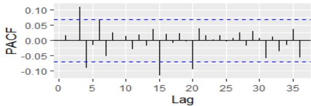
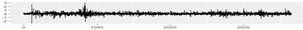
Forex USD/INR ARIMA residuals
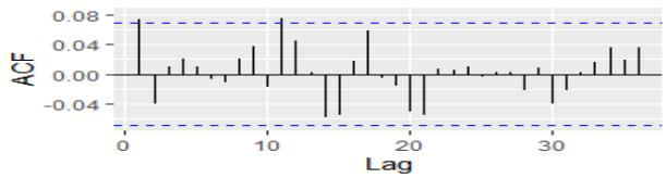
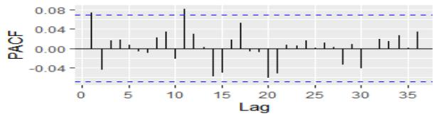
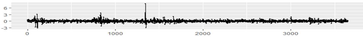
Forex CHF/INR ARIMA residuals
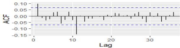
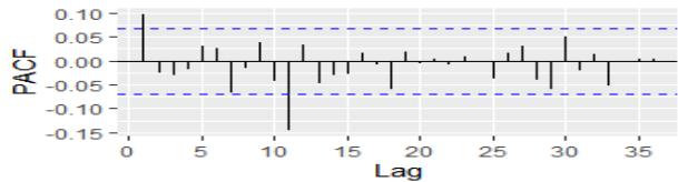
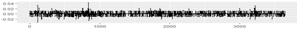
Forex YAN/INR ARIMA residuals
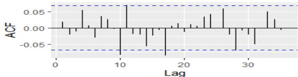
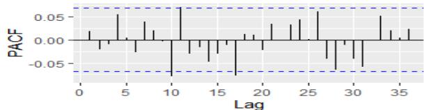
Figure 1.2.1: Residual Plots of the Daily Exchange Rates between USD/INR, GBP/INR, CHF/INR and JPY/INR
Observation of above Residual plots of the daily exchange rates between USD/INR, GBP/INR, CHF/INR and JPY/INR all are in the form of non-stationary, so we preferred ARCH and GARCH Models to test the diagnostic checking.
### f) ARCH, GARCH Comparison and Analysis
We shall be developing two types of models (ARCH - autoregressive conditional heteroskedastic model, GARCH - generalized autoregressive conditional heteroskedastic model and compare them in order to find the best model.
## i. Arch Analysis
Table 1.2.1: Chi-Squared and P-Values for the Fitted Model based on Daily Exchange Rates between USD/INR, GBP/INR, CHF/INR and JPY/INR
<table><tr><td></td><td>Chi-squared</td><td>p-value</td></tr><tr><td>USD/INR</td><td>200.77</td><td>; 2.2e-16</td></tr><tr><td>GBP/INR</td><td>41.134</td><td>=1.422e-10</td></tr><tr><td>CHF/INR</td><td>97.26</td><td>; 2.2e-16</td></tr><tr><td>JPY/INR</td><td>70.278</td><td>; 2.2e-16</td></tr></table>
Small p-values (less than 0.05) suggest that the data is stationary and doesn't need to be differenced. From Table 1.2.1 above, it is clearly seen that all the p-values of ADF test are less than 0.05, suggesting that the series of the foreign exchange rates of USD/INR, GBP/INR, CHF/INR and JPY/INR are stationary in mean but not in variance. Also, the USD/INR, GBP/INR, CHF/INR and JPY/INR foreign exchange rates show a clear evidence of ARCH effect since the p-values of Chi-square test are less than $\alpha = 0.05$. This signifies that the variances of the foreign exchange rates are nonconstant for all the periods specified. The Box and Jenkins procedure is applied to the variance series ( $Zi^2$ ) obtained from difference logged series of the closing prices which will lead to the model building process.
## ii. Garch Analysis
The model building procedures begins with the identified GARCH processes for the USD/INR, GBP/INR, CHF/INR and JPY/INR foreign exchange rates. The GARCH process based on following tests for checking its diagnostic Jarque Bera Test, Box-Ljung test. From Table 1.2.6, GARCH (1,1) process was identified for USD/INR foreign exchange rates, GARCH(1,1) process was identified for GBP/INR foreign exchange rates, GARCH (2,2) process was identified for CHF/INR foreign exchange rates and GARCH (1,1) process was identified for JPY/INR foreign exchange rates.
Below table present the GARCH processes and their parameters for USD/INR, GBP/INR, CHF/INR and JPY/INR foreign exchange rates.
Table 1.2.1: Summary of Garch Model Fit for USD/INR, GBP/INR, CHF/INR and JPY/INR Foreign Exchange Rates
<table><tr><td>Countries</td><td>Model</td><td colspan="4">Parameters</td></tr><tr><td></td><td>Identified</td><td>α0</td><td>α1</td><td>β1</td><td>β2</td></tr><tr><td>USD/INR</td><td>GARCH(1,1)</td><td>0.0020391</td><td>0.0642354</td><td>0.9040804</td><td>NIL</td></tr><tr><td>GBP/INR</td><td>GARCH(1,1)</td><td>0.018310</td><td>0.084582</td><td>0.841950</td><td>NIL</td></tr><tr><td>CHF/INR</td><td>GARCH(2,2)</td><td>0.0041388</td><td>0.1077998</td><td>0.2238257</td><td>0.6525444</td></tr><tr><td>JPY/INR</td><td>GARCH(1,1)</td><td>2.259e-05</td><td>5.000e-02</td><td>5.000e-02</td><td>NIL</td></tr></table>
The volatility model identified for USD/INR, GBP/INR, CHF/INR and JPY/INR foreign exchange rates are:
$$
\sigma_ {\mathrm {t}} ^ {2} = 0. 0 0 2 0 3 9 1 + 0. 0 0 2 0 3 \mathrm {Z} _ {\mathrm {t} - 1} ^ {2} + 0. 9 0 4 0 8 0 4 \sigma_ {\mathrm {t} - 1} ^ {2} \qquad \dots (5)
$$
$$
\sigma_ {\mathrm{t}} ^ {2} = 0.0 1 8 3 1 0 + 0.0 8 4 5 8 2 \mathrm{Z} _ {\mathrm{t - 1}} ^ {2} + 0.8 4 1 9 5 \sigma_ {\mathrm{t - 1}} ^ {2} \qquad \dots (6)
$$
$$
\sigma_ {\mathrm {t}} ^ {2} = 0. 0 0 4 1 3 8 8 + 0. 1 0 7 7 9 9 8 \mathrm {Z} _ {\mathrm {t} - 1} ^ {2} + 0. 2 2 3 8 2 5 7 \sigma_ {\mathrm {t} - 1} ^ {2} + 0. 6 5 2 5 4 4 4 \sigma_ {\mathrm {t} - 1} ^ {2} \dots (7)
$$
$$
\sigma_ {\mathrm{t}} ^ {2} = 2.259\mathrm{e} {-} 0 5 + 5.000\mathrm{e} {-} 0 2 \mathrm{Z} _ {\mathrm{t} - 1} ^ {2} + 5.000\mathrm{e} {-} 0 2 \quad \sigma_ {\mathrm{t} - 1} ^ {2} \qquad \dots (8)
$$
Table 1.2.2: Evaluation of Garch Model Fit for USD/INR Foreign Exchange Rates
<table><tr><td>GARCH(1,1)</td><td colspan="3">Parameters</td></tr><tr><td></td><td>α0</td><td>α1</td><td>β1</td></tr><tr><td>Standard Error</td><td>0.0001203</td><td>0.0043000</td><td>0.0050571</td></tr><tr><td>t-value</td><td>16.95</td><td>14.94</td><td>178.78</td></tr><tr><td>Pr((>—t—)</td><td><2e-16</td><td><2e-16</td><td><2e-16</td></tr></table>
Table 1.2.3: Evaluation of Garch Model Fit for GBP/INR Foreign Exchange Rates
<table><tr><td>GARCH(1,1)</td><td colspan="3">Parameters</td></tr><tr><td></td><td>α0</td><td>α1</td><td>β1</td></tr><tr><td>Standard Error</td><td>0.002088</td><td>0.004876</td><td>0.012585</td></tr><tr><td>t-value</td><td>8.77</td><td>17.34</td><td>66.90</td></tr><tr><td>Pr((>—t—)</td><td><2e-16</td><td><2e-16</td><td><2e-16</td></tr></table>
Table 1.2.4: Evaluation of Garch Model Fit for CHF/INR Foreign Exchange Rates
<table><tr><td>GARCH(1,1)</td><td colspan="4">Parameters</td></tr><tr><td></td><td>α0</td><td>α1</td><td>β1</td><td>β2</td></tr><tr><td>Standard Error</td><td>0.0005061</td><td>0.0072744</td><td>0.0537764</td><td>0.0507097</td></tr><tr><td>t-value</td><td>8.177</td><td>14.819</td><td>4.162</td><td>12.868</td></tr><tr><td>Pr((>—t—)</td><td>2.22e-16</td><td>< 2e-16</td><td>3.15e-05</td><td>< 2e-16</td></tr></table>
Table 1.2.5: Evaluation of Garch Model Fit for JPY/INR Foreign Exchange Rates
<table><tr><td>GARCH(1,1)</td><td colspan="3">Parameters</td></tr><tr><td></td><td>α0</td><td>α1</td><td>β1</td></tr><tr><td>Standard Error</td><td>3.782e-06</td><td>6.694e-03</td><td>1.495e-01</td></tr><tr><td>t-value</td><td>5.973</td><td>7.470</td><td>0.334</td></tr><tr><td>Pr((i—t—)</td><td>2.33e-09</td><td>8.04e-14</td><td>0.738</td></tr></table>
Table 1.2.6: Diagnostic Tests of Garch Model Fit for USD/INR, GBP/INR, CHF/INR and JPY/INR Foreign Exchange Rates
<table><tr><td>Countries</td><td colspan="2">Jarque Bera Test</td><td colspan="2">Box-Ljung test</td></tr><tr><td></td><td>Chi squared</td><td>p-value</td><td>Chi squared</td><td>p-value</td></tr><tr><td>USD/INR</td><td>21112</td><td>; 2.2e-16</td><td>7.5815</td><td>0.005897</td></tr><tr><td>GBP/INR</td><td>3442.1</td><td>; 2.2e-16</td><td>1.7723</td><td>0.1831</td></tr><tr><td>CHF/INR</td><td>234670</td><td>; 2.2e-16</td><td>0.0041978</td><td>0.9483</td></tr><tr><td>JPY/INR</td><td>2310.1</td><td>; 2.2e-16</td><td>7.6918</td><td>0.005547</td></tr></table>
g) Volatility USD/INR, GBP/INR, CHF/INR and JPY/INR Foreign Exchange Rates
The volatility is measured by the conditional standard deviation and it is presented in figure 1.2.2
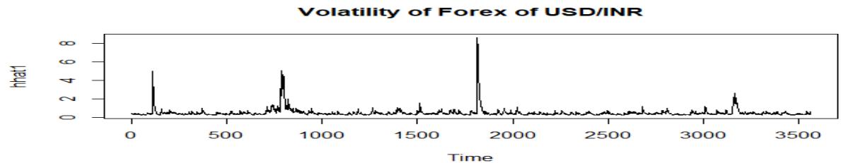
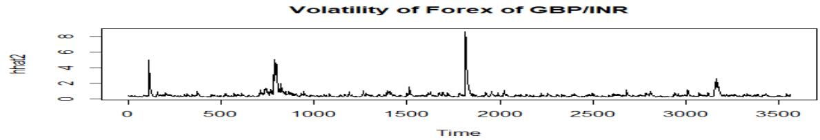
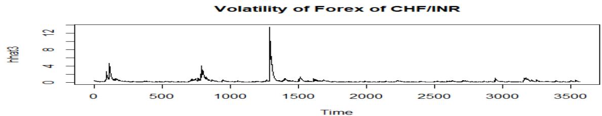
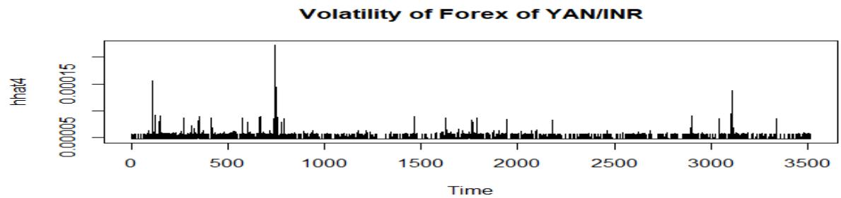
Figure 1.2.2: Conditional Standard Deviation Plot of USD/INR, GBP/INR, CHF/INR And JPY/INR Foreign Exchange Rates
## III. CONCLUSION
1. The test p-values from tables 1.2.1 (shown in the second column) are more than $5\%$, so in this model there is no ARCH effect, meaning that we have a good model.
2. From the p-value of the Jarque - Bera test we can state that the residuals are not normally distributed, which is not desirable. So, the only problem of the model is that the residuals are not normally distributed. The volatility is measured by the conditional standard deviation and it is presented in figure 1.2.2
3. The Box-Ljung test indicates that the ARCH (1) model is dynamically adequate with white noise error.
4. The volatility experienced by the insurance returns series were modeled using univariate Generalized Autoregressive Conditional Heterkedastic (GARCH) model and observed that GARCH (1,1) was identified as the best model for USD/INR and GBR/INR and YAN/INR. GARCH(2,2) was identified as the best model for USD/INR CHF/INR.
5. The Jarque Bera Test indicates the USD/INR, GBP/INR, CHF/INR and JPY/INR foreign exchange rates are significant.
6. The Box-Ljung test indicates that the USD/INR and JPY/INR foreign exchange rates are significant remaining GBP/INR, CHF/INR foreign exchange rates are insignificant.
7. The study has shown that GARCH models are better models for analyzing foreign exchange rates data.
Generating HTML Viewer...
References
12 Cites in Article
Z Alam,A Rahman (2012). Modelling Volatility of the BDT/USD Exchange Rate with GARCH Model.
C Babu,B Reddy (2014). Selected Indian stock predictions using a hybrid ARIMA-GARCH model.
Guillermo Benavides (2006). Predictive Accuracy of Futures Options Implied Volatility: The Case of the Exchange Rate Futures Mexican Peso-U.S. Dollar.
Tim Bollerslev (1986). Generalized autoregressive conditional heteroskedasticity.
K Dinesh,Sharma,H Hota,Kate Brown,Richa Handa (2021). Integration of genetic algorithm with artificial neural network for stock market forecasting.
Robert Engle (1982). Autoregressive Conditional Heteroscedasticity with Estimates of the Variance of United Kingdom Inflation.
Rodolfo Emerson,João Abraham,Gilberto Mendes Dos Reis,Oduvaldo Vendrametto,Pedro Luiz De Oliveira,Costa Neto,Rodrigo,Carlo Toloi,Aguinaldo Eduardo De Souza,Marcos De,Oliveira Morais (2020). Time Series Prediction with Artificial Neural Networks: An Analysis Using Brazilian Soybean Production.
H Glyn (2014). Value-at-Risk:.
J Hamilton (1994). Time Series Analysis.
Y Musa,M Tasi'u,B Abubakar (2014). Forecasting of Exchange Rate Volatility between Naira and US Dollar Using GARCH Models.
V Pacelli (2012). Road Crew.
A Sharma,R Vijay,G Bodhe,L Malik (2016). An adaptive neuro-fuzzy interface system model for traffic classification and noise prediction.
No ethics committee approval was required for this article type.
Data Availability
Not applicable for this article.
How to Cite This Article
Boina Jhansi Rani. 2026. \u201cForecasting Foreign Exchange Rates of Different Countries using Non Linear Models\u201d. Global Journal of Science Frontier Research - F: Mathematics & Decision GJSFR-F Volume 22 (GJSFR Volume 22 Issue F5).
Explore published articles in an immersive Augmented Reality environment. Our platform converts research papers into interactive 3D books, allowing readers to view and interact with content using AR and VR compatible devices.
Your published article is automatically converted into a realistic 3D book. Flip through pages and read research papers in a more engaging and interactive format.
Our website is actively being updated, and changes may occur frequently. Please clear your browser cache if needed. For feedback or error reporting, please email [email protected]
Thank you for connecting with us. We will respond to you shortly.