## I. INTRODUCTION oT has enabled us to develop a new generation of intelligent systems which had not been possible previously. The ability to connect every single entity and object in the physical world to the internet, through a mixture of communication protocols and techniques has applications in several domains. From industrial usage to smart city management systems [15] [16], IoT has infiltrated all aspects of our lives. Since IoT-based infiltrated all aspects of our lives. Since IoT-based applications demonstrated their capacity to enhance the quality of our lives, their pace of evolution has increased. Meanwhile, several concerns and challenges have been raised; here a primary problem is how to provide the required energy for these flourishing applications? Consider a smart city management system that comprises an enormous number of heterogeneous nodes that can sense and measure a mixture of vital system parameters. IoT nodes are mostly equipped with inexpensive and limited batteries which recharging and replacing them would not be practical or even possible. These Nodes are randomly placed in a large-scale context of a city and can have a distance of more than 2000 meters from the base station. Collecting information from these nodes will be costly in terms of energy, especially by increasing the required communication distance [17]. Additionally, a variety of other environmental constraints and limitation exists which must be considered. Clustering has been identified as a suitable solution for solving the challenge of long-distance data transmission [17] [18]. Unfortunately, this solution is complicated due to several parameters that should be considered. Most of these parameters are in contrast with each other. Hence, their simultaneous optimization would be difficult or sometimes impossible. In recent years, many valuable works have been done in this region that each of them considers a combination of parameters in different ways. In the following, we present five categories to provide a better understanding of reviewed solutions. ### a) Centralized or Distributed Centralized clustering algorithms are solutions in which the base station collects general network information, performs clustering, and finally informs the nodes. The 2 base station needs to collect general network information consists of different node's properties such as id, position, energy level, buffer size, data packet length, and so on; This information is applied for clustering the network. Although the effectiveness of this type of solution has been proven; using these approaches in heterogeneous crowded networks would not be practical since the base station have to gather and process large volumes of data which would be time-consuming and inefficient. Several protocols are located in this category, for instance, Stable-Aware Evolutionary Routing Protocol (SAREP) [1], at the beginning of this approach nodes are required to inform the base station of their id, position, and energy level. Then, N solution will be generated by the base station in each of which nodes with a high amount of residual energy have a higher chance to be picked as a cluster head. Each of these solutions presents a different network clustering strategy. An objective function will be utilized to evaluate a produced solution. After assessing each solution, the base station collects the best ones as next-generation parents. This process will continue until achieving a certain value of the objective function or till we produce and evaluate a certain number of generations or by reaching a defied limited execution time. [2] presented a DPSO-Based clustering routing algorithm that utilizes a two-field structure to produce experimental sequences. In other words, in this DPSO-Based solution, a set of random structures of the network (particles) is generated as the solution that each of which represents a clustering strategy. When the network information-gathering phase is completed, the base station collects $h^* 2$ nodes with the highest energy level as the cluster head candidates. Then each particle picks its cluster heads from this collection and randomly assigns them member nodes. Produced particles will be evaluated; consequently, the acceleration and success of the solutions will be updated. In this approach, the best solution is applied to orient new solutions. UMBIC [3] is an unequal multi-hop balanced immune clustering protocol that applies the MOIA algorithm, to collect an optimal number of nodes with the highest energy as the cluster head in a centralized manner. Then, the rest of the cluster formation process and building routing tree will be done by nodes cooperation; the main goal of this phase is to minimize communication costs and discard duplicate data overhead. As a powerful optimization tool, swarm intelligence has been employed in a variety of useful approaches such as SMO [4]. In this work, the problem of optimal clustering is considered as a Boolean problem so that a binary spider monkey optimization solution is presented to find the optimal solution. Briefly, SMO attempts to simulate search-and-find behavior among a group of spider monkeys. In this strategy, each solution considers as a spider monkey, and evaluation will be performed based on four objectives. Ultimately, each of these four objectives has a specific pre-defined weight that explicates the importance of each objective. LEACH [5] has been known as a fundamental algorithm for clustering IoT networks; several editions and versions have been proposed on this approach, WHCBA [6] is one of these editions. Operations of this approach are inspired by the actions of a group of bats during hunting. In this population-based solution, parameters such as the position of the bats, acceleration, frequency, propagation rate, and intensity are effective in the exploration of the optimal solution. Besides, after each solution generation, the best one will be applied to calculate the acceleration for future stages. In this approach, the objective function is a function of the standard deviation of the distance between the member nodes and the cluster head. The ultimate goal of such a consideration is to achieve the optimal solution with the minimum inter-cluster distance. Central-Id strategy is also adopted for producing new solutions. In this strategy, the farthest and closest nodes to the cluster head are picked and a search is performed to find the hidden nodes which are located within the aforementioned distance. BBO: EEEA [7] is another Si-based work in this context. After network information gathering, the base station produces N random solutions named habitant, each of which will be evaluated to calculate Habitat Suitability Index (HSI). Produced solutions will be prioritized based on their HSI and the emigration and immigration rate of each habitat is measured to be used in the production of next-generation solutions. In the biogeography optimization algorithm, migration is considered the main activity to produce the optimal solution. In this approach, the roulette wheel selection mechanism has been adopted to choose the habitat and migrate to it; Migration is used to generate new solutions. To produce more diversity, the mutation rates will adjust dynamically. Ultimately, after the production of new solutions, the immigration and emigration rate of each habitat are recalculated. To summarize, we can say most of the centralized Si-based approaches in this context, have a genetic-like functionality in producing N different solutions, evaluating them, selecting parents, and finally producing new generations. Although centralized approaches have demonstrated their skill in finding the optimal solution, they aren't suitable for large-scale IoT networks such as smart cities; which would consist of more than 5000 nodes. Due to their dependency on accessing global network information and its time-consuming mechanism for generation, composition, and evaluation of new solutions. This is where distributed solutions come in handy with large, scalable networks which have to achieve an optimized solution by considering time and energy constraints. 3 In Distributed approaches, IoT nodes are responsible to shape the clusters. In these methods, nodes are interacting and collaborating to produce a single optimal global answer. In this way, they do not require to send their local information fully to the base station and wait for the clustering result. The common skeleton of these approaches is consisting of these sub-phases; 1) Neighbor node discovery phase. 2) Cluster head competition phase. 3) Shaping clusters phase. 4) Cluster optimization phase. 5) Building a data transportation path phase. HUCL [8], EADUC [9], HEEC [10], HCD [11] are some of the proposed methods in this category. Although the above algorithms follow a similar structure they proposed diverse formula for node radius, waiting time (TW), and relay node evaluation calculation by considering different parameters which brought diversity in the final achieved answer. ### b) Equal or Unequal Clusters Regularly, Cluster radius can be categorized into three groups; 1) non-defined radius. 2) Defined and equal radius. 3) Defined and unequal radius. Non-defined radius: BBO: EEEE [7] is one of the strategies that do not consider a certain limited radius for cluster head. In general, distributed approaches can't be placed in this category. In other words, the neighbor node discovery phase has required distributed methods to define a specific radius for nodes to set a border for node communication and cooperation. Defined and Equal Radius: Although fixing an equal radius for clusters seems to be a practical solution for load balancing in homogenous IoT networks; it still has a negative aspect when we utilize multi-hop data transferring mechanism. In such situation, cluster nodes that are located next to the base station have to carry a lot of loads; which eventually leads to the energy hole problem near the base station and consequently reduces network coverage. To deal with this problem, the unequal cluster radius has been proposed. Table I: Categorized Reviewed IoT Clustering Algorithms <table><tr><td>Approach</td><td>Inter Cluster Layering</td><td>Inner Network Layering</td><td>Assistance Node Usage</td><td>Equal Or Unequal</td><td>Centralized Or Distributed</td></tr><tr><td>SAREP[1]</td><td>-</td><td>-</td><td>-</td><td>Unequal</td><td>Centralized</td></tr><tr><td>DPSO[2]</td><td>-</td><td>-</td><td>-</td><td>Unequal</td><td>Centralized</td></tr><tr><td>UMBIC[3]</td><td>-</td><td>-</td><td>VCH</td><td>Unequal</td><td>Centralized</td></tr><tr><td>SMO[4]</td><td>-</td><td>+</td><td>-</td><td>Unequal</td><td>Centralized</td></tr><tr><td>WHCBA[6]</td><td>-</td><td>-</td><td>-</td><td>Unequal</td><td>Centralized</td></tr><tr><td>BBO:EEEA[7]</td><td>-</td><td>-</td><td>-</td><td>Unequal</td><td>Centralized</td></tr><tr><td>HUCL[8]</td><td>-</td><td>+</td><td>-</td><td>Unequal</td><td>Distributed</td></tr><tr><td>EADUC[9]</td><td>-</td><td>+</td><td>-</td><td>Unequal</td><td>Distributed</td></tr><tr><td>HEEC[10]</td><td>+</td><td>+</td><td>ACH</td><td>Unequal</td><td>Distributed</td></tr><tr><td>HCD[11]</td><td>+</td><td>+</td><td>ACH</td><td>Unequal</td><td>Distributed</td></tr></table> Defined and Unequal Radius: The unequal cluster radius has been proposed to tackle the energy hole problem. In this solution to overcome high load near the base station, the nodes which are positioned nearby the base station will have a smaller radius. HUCL [8] is a sample of this class. ### c) Usage of Assistant Nodes Assistant nodes selection can be employed to minimize the energy depletion of cluster heads and also member nodes. The assistant nodes can be classified into two categories; 1) ACH. 2) VCH. ACH: These nodes are placed within a limited radius of the cluster head and are required to collect and aggregate data from members; they ultimately forward aggregated data to the related cluster head. Thus, not only inter-cluster communication distance will be minimized but also cluster heads need to waste less energy for data receiving and aggregation. HCD [11] is a sample of this category. VCH: UMBIC [3] is an example that has employed VCH nodes. These nodes are selected as substitutes for the cluster heads so that if the cluster head energy is dropped under a defined threshold; it could be replaced immediately without any additional processing. Employing this kind of assistance nodes will be essential especially for long-distance networks that when a cluster head dead occurs, member nodes are required to transfer their data directly to the base station which causes quick energy depletion. ### d) Utilizing Inner-network Layering In general, we can categorize mentioned algorithms into these groups; 1) Two-layered networks. 2) Four-layered networks. Two-Layered Networks: EADUC [9] simply defined a predefined threshold. So that, we can divide the network into two layers. The first layer comprises nodes that are placed near the base station. To overcome the energy hole problem these nodes are not permitted to pick a relay node. Four-Layered Networks: Nodes that are located in the farther layers have a greater radius in comparison with the ndes that are placed in lower layers. On the other hand, this layering makes it possible to construct a data transmission path by avoiding the loop. HCD [11] is a sample of this category. ### e) Utilizing Intra-Cluster Layering Due to the remarkable performance of inner-network layering, some solutions decided to apply this model for layering clusters as well as networks. Based on this idea, the cluster heads can share their data load among nodes that are located in the first layer. This mechanism is adopted for finding node assistants. HEEC [10] is an example of these algorithms. ## II. SYSTEM MODEL In this section, we present a real word smart city IoT network platform named SmartSantander; which inspired our performed simulation. SmartSantander [12] is a city scaled IoT project that has followed two principal aims: First, With the expansion of urbanization, city management is no longer as simple as it uses to be, and the former conventional systems are not proper for assisting city administrators; to make right decisions and perform timely and decent actions. By extending an efficient IoT platform, now it is possible to develop and present a varied range of services for citizens to improve the quality of resident's life. Second, to create a platform for researchers and developers for testing their IoT applications and services, in a real-world IoT platform. Smart Santander platform is composed of more than 20,000 indoor and outdoor IoT heterogeneous nodes which have been distributed on a city scale. These nodes can be utilized for multiple purposes; 1) Environmental monitoring. 2) Outdoor parking area management. 3) Parks and gardens irrigation. Three proposed applications Are some of the applications that can be implemented by applying this platform and has adopted a 3-tiered architecture, contains: ### 1) IOT Node Which are typical IoT nodes. #### 2) Repeaters Are IoT nodes that not only sense environmental parameters and send their prepared data to the base station but also forward other node's data. The communication between repeaters and IoT nodes performs through the 802.15.4 protocol which its range is limited between 10 to 100 meters [13]. So that we have employed this restriction in our simulations to achieve an estimation near the real world. #### 3) Gateways Both regular IoT nodes and repeaters are configured to send their data to gateways. finally, gateways send data to other machines or data centers. In this architecture, several gateways have been used in the environment to reduce data transformation distance. The following assumptions are made for our system model: - Nodes are distributed randomly and are stationary. - Nodes are configured to send their data to the nearest gateway. - Nodes are heterogeneous in terms of energy, produced data packet length, and buffer size. - Buffer limitation forces to forward data to the gateway by buffer filling event and ultimately, clear buffer to be able to accept new data from cluster members. - The node buffer's size is assumed to be 3 times more than each node's data packet length. - The maximum radius node is assumed to be 100 meters. We utilize a radio model same as [11], [14]. Here, consumed energy for transferring K bits data through dij distance can be calculated using the following equation. $$ E _ {T X} (i, K, d _ {i j}) = \left\{ \begin{array}{l l} E _ {e l e c} K + E _ {f s} K d _ {i j} ^ {2} & d _ {i j} \leq d _ {0} \\ E _ {e l e c} K + E _ {m p} K d _ {i j} ^ {4} & d _ {i j} > d _ {0} \end{array} \right. \tag {1} $$ dij is the Euclidean distance between two nodes; d0 is a threshold distance that can be calculated by employing the following equation. $$ d _ {0} = \sqrt {\frac {E _ {f s}}{E _ {m p}}} \tag {2} $$ Finally, consumed energy for receiving K bits data can be calculated using (3). $$ E _ {R X} (i, K) = E _ {e l e c} K \tag {3} $$ 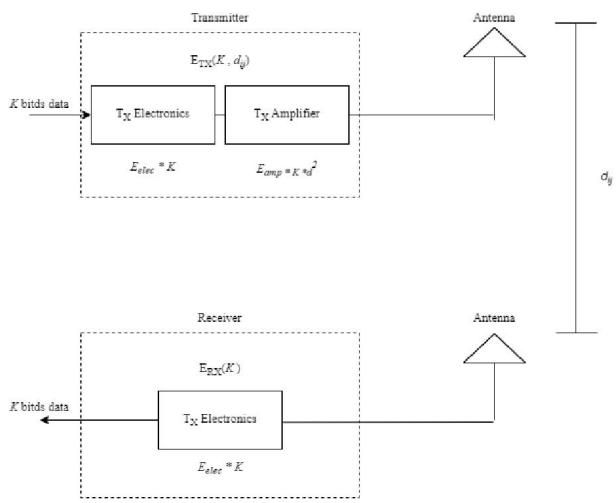 Fig. 2: IoT Radio Model. ## III. PERFORMED IMPROVEMENT With the rapid expansion of IoT applications, various challenges such as energy optimization and scalability have been considered. These problems are further complicated by considering several real-world constraints, such as energy, time, communication radius, and buffer size restrictions which are often in conflict with each other. During recent years several notable solutions have been introduced to face these concerns; each of them is different in terms of the combination of considered parameters and limitations. Here we present an effective improvement on the existing energy-aware distributed unequal clustering protocol (EADUC) algorithm. Our presented method is appropriate for clustering heterogeneous, large-scale IoT networks. Our recommended improvement attempts to enhance network lifetime by minimizing the number of dead nodes and consumed energy through utilizing three main enhancements: a) Neighbor Node Discovery Phase. b) Optimizing Clusters Phase. c) Assistance Node Selection Phase. Considering a smart city network that consists of more than 2000 heterogeneous nodes; gathering global network information, constructing and evaluating solutions, reproduction of new solutions generations, and ultimately providing an optimal answer would be time-consuming especially when a mixture of parameters should be considered. Thus, centralized strategies are not appropriate due to their time-consuming processes. However, distributed IoT clustering approaches are suited for networks with a considerable number of nodes, particularly under time restraints. Our distributed approach is consisting of six sub-phases: 1) Neighbor node discovery phase. 2) Cluster head competition phase. 3) Shaping clusters phase. 4) Cluster optimization phase. 5) Assistance node selection phase. 6) Building a data transportation path phase. We further describe these sub-phases in detail. ### a) Neighbor Node Discovery Phase In this sub-phase, each node gathers local network information by interacting with the neighbors; this information will be required for future decisions. Here, three significant questions must be answered: - What effects does radius computation have on energy efficiency? - How to calculate the optimal radius for a node? - How to lessen the energy consumption in the neighbor node discovery sub-phase? Above mentioned questions will be answered in this section one by one. As mentioned earlier, to tackle the energy hole challenge near the gateway, we produce clusters with unequal radius. Since by lessening the node's radius the number of neighbor nodes or future cluster members will be dropped. Hence, the radius of a node directly affects the load of the cluster, this fact has been used to coordinate the node's load by considering a variety of properties and restrictions such as 1) node's current energy. 2) node's network position. 3) node's buffer size. 4) node's data packet size. Moreover, cluster radius directly influences the number of clusters in the network. Since as the node's radius decreases more clusters will be needed to cover the same network area. In this situation, although the cluster head's load decreased; increasing the number of clusters will cause growth the total transmission distance and subsequently, total network consumed energy. In distributed clustering algorithms, optimal radius determination has been considered as a multi-objective optimization problem since there exists more than one parameter or objective for minimization or maximization; which some of them may have conflicts with each other.    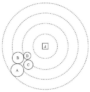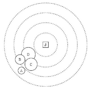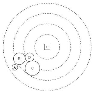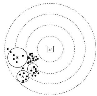 Fig. 3: Multi-Objective Radius Optimization. Assume four nodes: A, B, C, D; which are varied in terms of 1) Distance to the gateway. 2) Energy level. 3) Buffer size. 4) Area density. Suppose that We have considered four goals in node's radius optimization: - A: To minimize the radius of nodes that have less distance to the gateway. Consequently, we would be able to reduce the load of nodes near the gateway and prevent the energy hole problem. - B: To maximize the radius of nodes that have more residual energy or in other words have consumed less energy during previous rounds. Hence, we could lessen the load of nodes that have less remaining energy. 6 - C: To minimize the radius of nodes that have a smaller buffer size. - D: To minimize the radius of the nodes which are located in a dense area. Figure 4 is presenting our four radius optimization strategies and conflicts among them. For instance, in the first strategy A has the maximum radius since it has more distance to the gateway. However, in the second strategy A has the least radius since it has a lower energy level. As we stated node radius optimization has been considered as a multi-objective optimization problem in IoT distributed clustering approaches; due to its intent to minimize or maximize multiple parameters and achieving multiple conflict goals. Here, we utilized a decomposition multi-criteria optimization solution named weighted sum same as radius computation formula which is employed in EADUC [9]. These objective functions can be considered: To maximize the radius of nodes that have more distance to the gateway. Thus we would be able to lessen the load of nodes that are located near the gateway and prevent the energy hole problem. To this end, we used the (4) as an objective function that encounters the distance from the maximum value. (dmax - dmin) is the network length of the current gateway. The resulted value will be bounded between 0 and 1. For nodes that are located near the gateway this value is smaller. $$ Z_{5} = \frac{X-\max(X)}{\max(X)-\min(X)} = \frac{d_{max}-d(s_{j},BS)}{d_{max}-d_{min}} \tag{4} $$ To maximize the radius of nodes that have consumed less energy during previous rounds. Consequently, we could lower the load of nodes that have consumed more energy previously. Thus, we applied (5) as an objective function that expresses the relative proximity of each node energy value to its maximum energy. The resulted value will be bounded between 0 and 1. For nodes that have been wasted more energy this value is smaller. $$ Z _ {3} = \frac {X}{\max (X)} = \frac {E _ {r}}{E _ {\max }} \tag {5} $$ Ultimately, by multiplying each objective function by -1 or by subtracting the limit value (between 0 and 1) by 1; we can convert the minimization objective function to maximization or vice versa. The Rlmax is a predefined coefficient that directly affects the radius of nodes and maximizes our control on radius computation. When it comes to reducing energy consumption in the neighbor node discovery sub-phase; Restricting the number and the size of broadcasted packages will be profitable. As the result, here we have applied an improvement in the original EADUC approach. In regular neighbor node discovery strategies, each node broadcasts a request for information message in their restricted radius. Then, each node that hears this message will respond back by sending a packet containing its properties. consequently, if a node hears n requests for information message; it will send n packages in reply. Our applied strategy required a node to broadcast a replay packet only once and reduces the consumed energy from nETX to maximum ETX. Fig 4 is representing mentioned strategy. Fig 6 displays, our presented method, which can be split into two sub-steps: T1: This is the duration in which nodes broadcast the request for the information message. Each neighbor node will receive the message and saves the id and position of each received request in a list. So that in the next step it can increase its radius just in case to obtain the maximum required radius to answer the message once; temporary. Since our assumption considered the 802.15.4 protocol range limitation, we can be assured that this radius will never exceed 100 meters. T2: This is the duration in which each node checks its list to find the maximum necessitated radius to broadcast its information once. ### b) Cluster Head Competition Phase The primary purpose of this sub-phase is to collect optimal cluster heads by maximizing their opportunity to be selected. In this strategy, a waiting time will be set by each node. Nodes that have not received the head message till the end of their waiting time; will consider themselves as cluster heads and broadcast a head message in their radius to inform their neighbors. For maximizing the chance of optimal nodes to become a cluster head or minimize the waiting time of optimal nodes; this problem can be considered as an optimization problem. 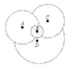To this end, a variety of node's properties can be considered:  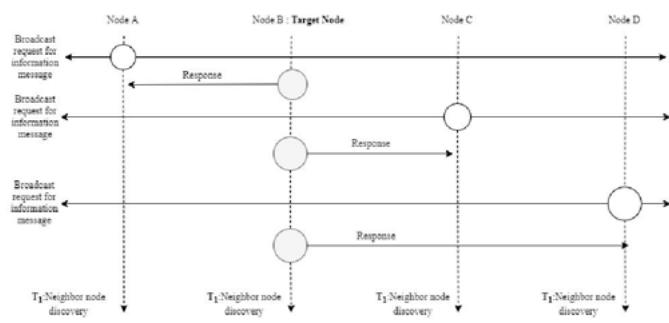 Fig. 4: Regular Neighbor Node Discovery. Node energy state, the proportion of average energy of the neighbors (6) and current node residual energy (7); can be considered as an objective function. consequently, nodes that have more energy in comparison to their neighbor average energy; have more chance to become a cluster head. $$ E _ {a v g \_ r e s} = \frac {\left(\sum_ {j = 1} ^ {m} s _ {j} E _ {r}\right)}{n b} \tag {6} $$ $$ Z _ {3} = \frac{X}{\operatorname* {m a x} (X)} = \frac{E _ {a v g - r e s}}{E _ {r}} \quad E _ {r} \geq E _ {a v g - r e s} $$ Or the amount of consumed energy (8), in this way we could maximize the chance of becoming cluster heads for nodes which, have lost less energy. $$ Z _ {3} = \frac{X}{\operatorname* {m a x} (X)} = \frac{E _ {r e m}}{E _ {i n t}} \tag{8} $$ The number of times that a node acts as a cluster head, by applying this parameter, we can improve the chance of becoming a cluster head for nodes that have not spent much energy as a cluster head. 8 The number of neighbor nodes, this parameter can be employed to coordinate the load balancing among the nodes.  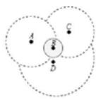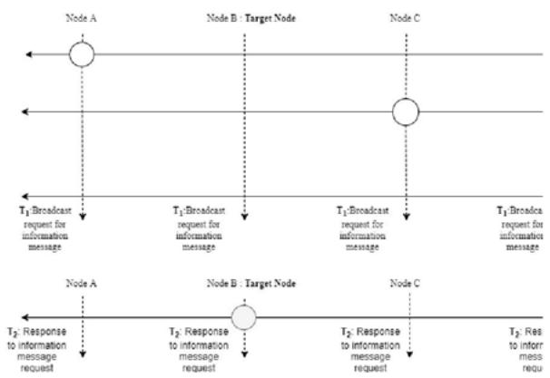 Fig. 5: Proposed Neighbor Node Discovery. ### c) Shaping Clusters Phase In distributed approaches after completing the cluster head competition phase; entire the network is covered by clusters. So that each alive node has the rule of cluster head or member node. In the cluster formation phase, member nodes are required to select an appropriate cluster head from the developed cluster head list. To reduce the intra-cluster distance and consequently consumed intra-cluster communication energy. Regularly, member nodes are expected to pick the cluster head with the least distance. Hence, a cluster head's load highly depends on the density of the located area, radius, and Tw of its surrounded nodes. To enforce more control on load balancing here we have applied an additional phase named the cluster optimization phase. ### d) Clustering Optimization Phase To enhance better load balancing, here we have implemented our improvement by utilizing a well-known swarm intelligence algorithm (SI), named Biogeography-based optimization (BBO) [19] in a distributed manner. BBO is an intelligence optimization algorithm introduced in 2008 by Dan Simon. The basic idea is based on this central question, how various plant and animal species are distributed in geographical areas. As a fact, we know that animals tend to monopolize resources, so the ideal locality for them is a place with the lowest possible population. This performance of animals in emigrating from densely populated areas and immigration to sparsely populated areas is the basic idea of the BBO optimization algorithm; which can also assist us to achieve better load balancing in IoT clustering. To provide a better perception of our implementation, consider four nodes A, B, C, and D.D selected C as cluster head among its head list since it has the least distance. C has got the highest population among two other possible habitats so its emigration rate is higher than two other options. As a result, D has a high intend to leave C and find a new cluster or habitant that has a less population. 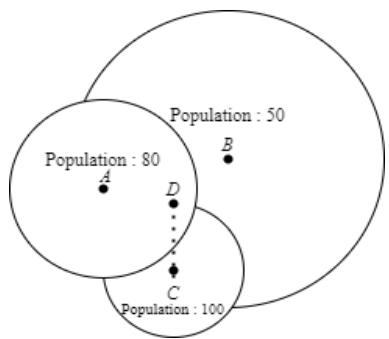 Fig. 6: Node possible habitants. This is our viewpoint in employing the BBO algorithm; in other words, by utilizing head list as a possible habitat list and BBO, each member node does immigration and 9 emigration to distribute load among possible habitats and achieve better load balancing. To this end after regular cluster shaping; each cluster head as a habitant calculates its current load and informs its member by broadcasting a small 32 bits message. Thus, each member node can compute the habitat suitability index (HSI) for each of the possible habitats in the head list. This HSI is an objective function that can improve cluster head load balancing. Here we considered three habitant suitability index (SIV) that forms our final HIS: The required energy to transfer the node's data packet. This suitability index has a direct relation to the distance. So, the nearest cluster head is the most proper option. Here we considered the distance to the minimum Etx needed as an SIV. $$ Z_{5} = \frac{X-\operatorname*{min}(X)}{\operatorname*{max}(X)-\operatorname*{min}(X)} = \frac{E_{tx}-\operatorname*{min}(E_{tx})}{\operatorname*{max}(E_{tx})-\operatorname*{min}(E_{tx})} $$ Our second suitability index can be considered as a constraint. Hence, we can convert our HSI to a constrained optimization problem. To this end here we defined load violation as a parameter that affects our final objective function. Our main goal is to keep the habitant's load less or equal to its buffer size. $$ V \{g (x) < g _ {0} \} = \left\{ \begin{array}{ll} 0 & g (x) \leq g _ {0} \\ \frac {g (x)}{g _ {0}} - 1 & g (x) > g _ {0} \end{array} \right. \tag {10} $$ Here $g_0$ is the buffer size constraint of habitant $x$ and $g(x)$ is the current load of habitant $x$. This load violation value will use as a penalty value which can be appended to the objective function and increased the value of the HSI in the minimization problem. Our third SIV attempts to prevent the accumulation of load in a habitat. Worst load violation is a parameter that shows load violation when the habitant accepts the maximum possible load. Here we apply (10) for violation computation but we considered $g(x)$ as the current habitant worst load. Ultimately, our HSI will be presented as follow: $$ \begin{array}{l} H S I = w _ {1} \left(\frac{E _ {t x} - \operatorname* {m i n} (E _ {t x})}{\operatorname* {m a x} (E _ {t x}) - \operatorname* {m i n} (E _ {t x})}\right) \\+ w _ {2} (\text{CurrentLoadViolation}) \tag{11} \\+ w _ {3} (\text{WorstloadViolation}) \\\end{array} $$ w1, w2, and w3 are weights that reveal the parameter importance. After calculating HSI, evaluated habitats will be sort in descending order. Ultimately, the immigration rate and emigration rate can be computed based on [19]. Although the BBO algorithm has been utilized in other centralized IoT clustering approaches previously; we were able to present a distributed usage of this algorithm which helps us not only get profits of its capabilities but also consider the time limitation in our network. In the other words, to present more controllable load balancing we permit our member nodes to reshape the clusters; utilizing their local information and BBO as a practical load balancing tool. On the other hand, we have been able to enforce buffer size constraints by employing a constrained objective function as HSI. ### e) Assistance Node Selection Phase To reduce energy dissipated in the urgent conditions that a cluster head dies or lost its energy more than the expected defined value. we have employed VCH assistant nodes selection. These nodes are selected as substitutes for the cluster heads so that if the cluster head died; it could be replaced immediately without any additional processing. Employing this kind of assistance nodes will be essential especially for long-distance networks when a cluster head dead happens, member nodes are required to transfer their data directly to the base station which causes quick energy depletion. To pick an appropriate VCH, each cluster head does member evaluation to find a VCH that has residual energy more than average member energy and has the least distance to the current cluster head ### f) Building A Data Transportation Path Phase Here a multi-hop strategy is adopted, to reduce communication distance between the cluster heads and the gateway. Same as the EADUC algorithm, a threshold distance named dist_th is defined. If a cluster head is placed in a distance less than dist_th; it is not allowed to pick a relay node; so that we can face the energy hole problem. To build a data transmission path, each cluster head broadcasts its information in its radius to inform other cluster heads. Each cluster head that receives this information; will save this data in a list so that it can evaluate each cluster head based on required relay energy and ultimately picks the one which needs less energy waste. 10 Fig. 8 A comparison of Average Cluster Head's Load Standard Deviation before and after improvement. 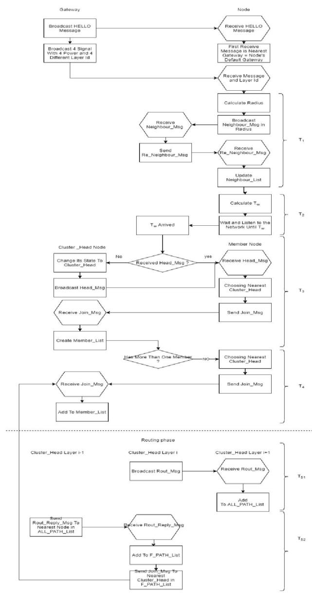 Fig.7: Flowchart of Presented Improved EADUC Algorithm. ## IV. EXPERIMENTAL AND PERFORMANCE ANALYSIS To carry out our simulation MATLAB R2019b has been employed. To present a more explicit analysis of our presented improvement. First, we consider a simple $200 \times 200$ square-shaped environment that includes 3,401 randomly distributed heterogeneous nodes; each of which is modified to interact with the nearest gateway. Table II and III demonstrates the network composition which has considered as our first scenario. Table II: Scenariosimulation Parameters <table><tr><td>Parameter</td><td>Value</td></tr><tr><td>Total Temperature Repeater Nodes</td><td>920</td></tr><tr><td>Total Light Repeater Nodes</td><td>353</td></tr><tr><td>Total Noise Repeater Nodes</td><td>558</td></tr><tr><td>Total Gases Repeater Nodes</td><td>443</td></tr><tr><td>Total Parking Sensor Nodes</td><td>337</td></tr><tr><td>Total Multimedia Nodes</td><td>750</td></tr><tr><td>Rlmax</td><td>10</td></tr></table> 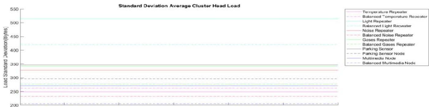 Fig. 8: A comparison of Average Cluster Head's Load Standard Deviation before and after improvement. In the homogeneous networks, load balancing can be simply measured by calculating the standard division of the cluster head's load. To this end, standard division can be calculated in a single round. Since the goal is to build clusters with the nearly same amount of load. However, in heterogeneous networks, each cluster load depends on its constraints, and their capacity is not comparable. To achieve this comparison possibility, here we present a measurement named standard division of average cluster head's load. To measure this parameter, in each round we calculate the average load of each cluster head types separately ultimately, we can compare this average for each type using standard division considering total rounds. Fig 9 illustrates the ability of our improvement in achieving load balancing in heterogeneous networks. Since the standard division of each cluster head type reduced successfully after applying our presented improvement. $$ \sigma i = \sqrt{\Sigma} \, |\mu i - \bar{x} i| \, 2 N j = 1 N $$ Formula (12) represents the standard division of cluster head type i, during N rounds of clustering and data transition. $\mu j$ is the average load of node type i in j-th round and $\overline{x}i$ is the average of average load for type i during all N rounds. Our simulation with examining scenario 1, shows a reduction in total load standard division from $2.0514\mathrm{e} + 03$ to $1.6926\mathrm{e} + 03$ after implementing BBO load balancing improvement; which reveals a decline near 17.49 percentage. Table III: Simulation Parameters Parameter <table><tr><td>Parameter</td><td>Value</td></tr><tr><td>Temperature RepeaterInitial Energy</td><td>5 J</td></tr><tr><td>Temperature Repeater Packet Size</td><td>300 bites</td></tr><tr><td>Temperature Repeater Buffer Size</td><td>300×3 bites</td></tr><tr><td>Light Repeater Initial Energy</td><td>6 J</td></tr><tr><td>Light Repeater Packet Size</td><td>500 bites</td></tr><tr><td>Light Repeater Buffer Size</td><td>500×3 bites</td></tr><tr><td>Noise Repeater Initialize Energy</td><td>7 J</td></tr></table> <table><tr><td>Noise Repeater Packet Size</td><td>400 bites</td></tr><tr><td>Noise Repeater Buffer Size</td><td>400×3 bites</td></tr><tr><td>Gases Repeater Initial Energy</td><td>8 J</td></tr><tr><td>Gases Repeater Packet Size</td><td>400 bites</td></tr><tr><td>Gases Repeater Buffer Size</td><td>400×3 bites</td></tr><tr><td>Parking Sensor Initial Energy</td><td>9 J</td></tr><tr><td>Parking Sensor Packet Size</td><td>200 bites</td></tr><tr><td>Parking Sensor Buffer Size</td><td>200×3 bites</td></tr><tr><td>Multimedia Node Initial Energy</td><td>10 J</td></tr><tr><td>Multimedia Node Packet Size</td><td>400 bites</td></tr><tr><td>Multimedia Node Buffer Size</td><td>400×3 bites</td></tr><tr><td>Eelec</td><td>50 nJ/bit</td></tr><tr><td>Efs</td><td>10 pJ/bit/m2</td></tr><tr><td>Emp</td><td>0.0013 pJ/bit/m4</td></tr><tr><td>EDA</td><td>5 nJ/bit/message</td></tr><tr><td>MiniSlot</td><td>20</td></tr><tr><td>MajorSlot</td><td>2</td></tr><tr><td>Rlmax</td><td>-</td></tr><tr><td>Packet Header Size</td><td>50 bites</td></tr><tr><td>I,E</td><td>1</td></tr><tr><td>α,β,</td><td>0.333</td></tr><tr><td>Total Gateways</td><td>25</td></tr><tr><td>W1</td><td>0.2</td></tr><tr><td>W2</td><td>0.4</td></tr><tr><td>W3</td><td>0.4</td></tr></table> To confirm the efficiency of our presented improvement, in a near-real word environment the second scenario is considered. Moreover, four other existing distributed clustering algorithms named EADUC, HCD, HUCL, and HEEC have been simulated using the same scenario parameters to perform a satisfactory comparison. To measure the performance of each approach four different parameters has been examined: ### 1) Total Network Remaining Energy Energy consumption is identified as a key restriction in prolonging network lifetime. This parameter has close dependencies with other network measures such as the number of cluster heads and cluster load that has made the optimization more complicated. However, by expanding cluster heads load will distribute more and reduced. This relation can be demonstrated in Fig 8 and fig 11. Here we have selected EADUC as the base algorithm to implement our performed improvement; since it has the least amount of cluster heads among the three other approaches. The following chart displays the performance of our improvement in energy efficiency; Our improved EADUC approaches were able to waste the least energy in contrast to the other four approaches. In comparison to the original EADUC by remaining network energy 56728.83, our improved approaches were able to keep 57631.79 which shows a 1.59 percent drop in energy consumption. 2) Total Number of Cluster Heads in Each Round 3) Total Number of Alive/Dead Nodes in Each Round The number of alive/dead nodes is the next essential criterion for prolonging network lifetime and preserving network coverage. The two following charts display the ability of our offered approach to decrease the ratio of losing nodes. 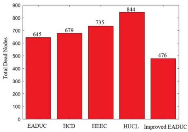 Fig. 13: Total Dead Nodes Scenario 2. Table III: Scenario 2 Simulation Parameters <table><tr><td>Parameter</td><td>Value</td></tr><tr><td>M×M</td><td>2000×2000</td></tr><tr><td>Total Temperature Repeater Nodes</td><td>1920</td></tr><tr><td>Total Light Repeater Nodes</td><td>1353</td></tr><tr><td>Total Noise Repeater Nodes</td><td>1558</td></tr><tr><td>Total Gases Repeater Nodes</td><td>1443</td></tr><tr><td>Total Parking Sensor Nodes</td><td>1377</td></tr><tr><td>Total Multimedia Nodes</td><td>1750</td></tr><tr><td>RImax</td><td>100</td></tr></table> ## V. DATA TRANSMISSION SIMULATION AND HETEROGENEOUS BUFFER SIZE With no doubt, heterogeneity is the primary property of an IoT real-world network. Since a typical IoT network may comprise hundreds of nodes, produced by different companies and with a variety of capabilities and constraints. Moreover, these heterogeneous nods may employ diverse communication protocols. This fact has made clustering optimization more complicated. So that, although several practical approaches have been introduced during recent years, not all of the heterogeneous properties and real-world network conditions have been considered by them. In this paper, we have considered a group of real-world attributes in our presented work and simulations: 1) Node's Energy Heterogeneity. 2) Node's Produced Packet Size Heterogeneity. 3) Node's Buffer Size Heterogeneity. 4) Limited Node Radius (Zigbee Communication Radius Constraint). 5) Clustering Execution Time Limitation.  Fig. 9: Network Energy in Scenario 2.  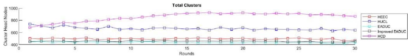Fig. 10: Total Cluster Heads Scenario 2.   Fig. 11: Total Alive Nodes Scenario 2. Fig. 12: Total Dead Nodes Scenario 2. In this section, we present our data transmission phase by considering buffer size constraint and packet size heterogeneity. In most of the data gathering mechanisms, TDMA be instructed to gather data from the farthest nodes first. Hence, data can properly be aggregated by intermediate nodes before forwarding to the gateway. In the other words, the node's defined slot time is related to its distance to the next-hop node. 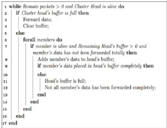 Fig. 14: Data Transition. Here to consider buffer limitation, we start data gathering from the farthest nodes. Consider node A in fig 14 as a cluster head; TDMA is set to collect data from nodes based on their distance to A. This data accepting by node A will continue until it reaches buffer size limitation. Then, to resume its process, node A is required to unload its buffer by transferring its collected data to the 13 next hop. Consequently, the buffer will be reset to accept the rest of the data. This procedure will be continuing as mentioned in pscode, until the rest of the data will be gathered or its energy be consumed completely. ## VI. CONCLUSION In this paper, first, we categorized our studied approaches based on a variety of properties; then based on the presented classification we selected distributed approaches as an appropriate clustering method for large-scale heterogeneous IoT networks. Due to their ability to present optimized solutions by utilizing local limited information promptly. Eventually, to perform our enhancement we selected EADUC approaches among three other existing distributed strategies. The main reason for our selection is the capability of EADUC to present the most energy conservation clustering solutions by employing the fewest amounts of cluster heads. Finally, we implement three main improvements to the selected strategy: ### a) Neighbor Node Discovery Phase Our performed enhancement can lessen the number of required messages and consequently wasted energy in this phase. ### b) Optimizing Clusters Phase Here we employed BBO as a practical tool for distributing loads among heterogeneous neighbor clusters. To orient the migrations based on heterogeneous limitations we have implemented a constrained optimization objective function as a habitat suitability index. ### c) Assistance Node Selection Phase We recognized two types of assistance nodes in the current presented approaches, as we have considered large-scaled long-distance IoT networks; missing cluster heads during the data transmission phase will cost a lot. Since by losing the cluster head, all members are required to send their data directly to the gateway; This will cause energy wastage. To assure the cluster structure we have employed VCH assistance node selection. So that by missing a cluster head it can immediately be replaced by other members with no further computation; hence the cluster structure will be maintained. Three cited advancements are presented in the EADUC algorithm to provide an optimized distributed clustering approach for heterogeneous IoT networks.

Generating HTML Viewer...

References

10 Cites in Article
(2014). 2014 IEEE World Forum on Internet of Things (WF-IoT).
Faisal Shaikh,Sherali Zeadally,Ernesto Exposito (2015). Enabling Technologies for Green Internet of Things.
Sauro Longhi,Davide Marzioni,Emanuele Alidori,Gianluca Di Buo,Mario Prist,Massimo Grisostomi,Matteo Pirro (2012). Solid Waste Management Architecture Using Wireless Sensor Network Technology.
Pritee Parwekar,Vyshnavi Nagireddy (2018). Comparative Analysis of SGO and PSO for Clustering in WSN.
N Mazumdar,S Roy,S Nayak (2018). A survey on clustering approaches for wireless sensor networks.
M Ergezer,D Simon,D Du (2008). Biogeography-based optimization.
V Deshpande,A Patil (2013). Energy efficient clustering in wireless sensor network using cluster of cluster heads.
O Younis,S Fahmy (2004). HEED: a hybrid, energy-efficient, distributed clustering approach for ad hoc sensor networks.
Pablo Sotres,Juan Santana,Luis Sanchez,Jorge Lanza,Luis Munoz (2017). Practical Lessons From the Deployment and Management of a Smart City Internet-of-Things Infrastructure: The SmartSantander Testbed Case.
Antonio Jara,Dominique Genoud,Yann Bocchi (2014). Short paper: Sensors data fusion for Smart Cities with KNIME: A real experience in the SmartSantander Testbed.
Explore published articles in an immersive Augmented Reality environment. Our platform converts research papers into interactive 3D books, allowing readers to view and interact with content using AR and VR compatible devices.
Your published article is automatically converted into a realistic 3D book. Flip through pages and read research papers in a more engaging and interactive format.
Our website is actively being updated, and changes may occur frequently. Please clear your browser cache if needed. For feedback or error reporting, please email [email protected]
Thank you for connecting with us. We will respond to you shortly.