## I. RADIO LINK IN FREE SPACE WITH TWO HALF-WAVE DIPOLE ANTENNAS In free space radio link between two identical resonant and perfectly matched half-wave dipole antennas the theoretical results, taking into account that the power gain is exactly equal to the directivity, are the following: Tx antenna theoretical power gain $G_{T} = 2.15$ (dBi) Tx antenna theoretical effective area $A_{eT} = 0.13\lambda^2$ Tx antenna theoretical effective length $L_{eT} = 0.3183\lambda$ Rx antenna theoretical receiving power gain $G_{R} = 2.15$ (dBi). Rx antenna theoretical receiving effective area $A_{eR} = 0.13\lambda^2$ Rx antenna theoretical scattering power gain $G_{s} = -0.85$ (dBi). Rx antenna theoretical scattering effective area $A_{es} = 0.065\lambda^2$ Rx antenna theoretical effective length $L_{eR} = 0.3183\lambda$ Tx antenna power gain $G_{T}$ in free space [2],\[3\]: $$ G _ {T} = 2. 1 5 (\mathrm {d B i}) $$ Rx antenna effective receiving area $A_{eR}$ definition [2],\[3\]: $$ A _ {e R} = W _ {R} / P _ {i} $$ In a simulation made up by means of a software program (WIPL-D) [6] and additional calculations for parameters not obtained by the software, the results are the following: For $\mathrm{f} = 300(\mathrm{MHz})$, $\lambda = 1(\mathrm{m})$, $\mathrm{r} = 100(\mathrm{m})$ $$ R _ {a T} = R _ {a R} = 7 1. 0 (\Omega), R _ {L} = 7 1 (\Omega), W _ {T} = 1 (\mathrm {W}). $$ Tx antenna power gain $G_{T} = 2.12$ (dBi). Tx antenna effective area $A_{eT} = 0.13(m^{2})$ Tx antenna effective length $L_{eT} = 0.3183(m)$ Tx Antenna factor $aF_{T73} = 15.97(dB / m)$ Tx Antenna factor $aF_{T50} = 17.61(dB / m)$ Rx antenna receiving power gain $G_{R} = 2.15$ (dBi). Rx antenna scattering power gain $G_{s} = -0.89$ (dBi). Rx antenna scattering effective area $A_{es} = 0.065(m^2)$ Rx antenna effective length $L_{eR} = 0.3183\lambda$ Rx antenna received current $I_{R} = 1.5$ E-4 (A). Rx antenna received voltage $V_{R} = 1.09$ E-2 (V). Rx antenna received power $W_{R} = 1.68$ E-6 (W). Rx Antenna factor $aF_{R73} = 15.97(dB / m)$ Rx Antenna factor $aF_{R50} = 17.61(dB / m)$ In this example, the Friis power budget is shown because for a perfect resonant and matched antenna the theoretical power gain or directivity are exactly the same [3]. In this case, the difference between directivity and gain is negligible or around 0.01 dB. Antenna efficiency is around 97 percent. Generally, losses are in the matching systems or in transmission lines but not in the antennas and must be computed separately. The transmission loss or site attenuation for a distance $r = 100$ (m) and for the transmitted power $W_{T} = 1$ (W), is: $$ A _ {w} = 1 0 \log W _ {R} = 1 0 \log 1. 6 8 E - 6 = - 5 7. 7 5 (d B) $$ The nondissipative free space attenuation, is: $$ A _ {F S} = 1 0 \log (\lambda / 4 \pi r) ^ {2} = - 6 1. 9 8 (d B) $$ Using the secondary or additional Friis equation [3] for the parameters in dB, results in: $$ G _ {T} + G _ {R} = A _ {w} - A _ {F S} = K (d B). $$ $$ G_{T} + G_{R} = 2.12 + 2.11 = 4.23 (dB). $$ $$ K = A_{w} - A_{FS} = -57.75 - (-61.98) = 4.23 (dB) $$ Friis power budget was corroborated because the antenna gains are exactly the space losses. Also, the power reciprocity principle from Schelkunoff and Friis [3] is confirmed, or: $$ A _ {e T} / g _ {T} = 0. 0 7 9 $$ $$ A _ {e R} / g _ {R} = 0. 0 7 9 $$ $$ A _ {e s} / g _ {s} = 0. 0 7 9 $$ All data were the result of calculations and not assigning any supposed value at the antenna gains as well as it can be obtained by power measurements [7], [8]. In a radio link in free space the Tx and Rx antennas have the area, gain and factor of the same value [2],[3]. It is important to verify in any radio link if the reciprocity principle is fulfilled, to be: $$ A _ {e T} / g _ {T} = A _ {e R} / g _ {R} = A _ {e s} / g _ {s} $$ ## II. RX HALF-WAVE DIPOLE ANTENNA IN FREE SPACE AND SHORT CIRCUIT Calculated by a software program (WIPL-D) [6] with the following data, for: $$ \begin{array}{l} \mathrm {f} = 3 0 0 (\mathrm {M H z}), \lambda = 1 (\mathrm {m}), \mathrm {r} = 1 0 0 (\mathrm {m}), \\R _ {a T} = R _ {e R} = 7 1. 0 (\Omega), R _ {L} = 0. 0 (\Omega), W _ {T} = 1 (\mathrm {W}). \\\end{array} $$ Tx antenna power gain $G_{T} = 2.13$ (dBi). - Tx antenna effective area $A_{eT} = 0.13(m^{2})$ - Tx antenna effective length $L_{eT} = 0.3183$ ( $m$ ). - Rx antenna receiving effective area $A_{eR} = 0.0(m^{2})$ - Rx antenna scattering power gain $G_{s} = 2.13$ (dBi). - Rx antenna scattering effective area $A_{es} = 0.13(m^2)$ - Rx antenna effective length $L_{eR} = 0.3183 \, m$. - Rx antenna received current $I_{R} = 3.1$ E-4 (A). - Rx antenna received voltage $V_{R} = 0.0$ (V). - Rx antenna received power $W_{R} = 0.0$ (W). - Rx antenna scattered power $W_{s} = 6.91$ E-6 (W). In his original book "ANTENNAS" Dr. John Kraus [2] took as scattering area $A_{es}$ the relation between the reradiated or scattered power $W_{s}$ and the incoming power density $P_{i}$ instead of calculating the scattering area $A_{es}$, that was suggested by Harald Friis [3], for the case of a transmitting or retransmitting antennas, according to the radiated numerical gain $g_{T}$ or scattered numerical gain $g_{s}$. This event was repeated incorrectly in several other antenna theory books. Using the scattered area by Dr. Kraus the scattered gain $G_{s}$ would acquire more than 8 (dBi) which is not possible for a simple half-wave dipole antenna in short circuit and free space. It can show calculations, that the maximum gain in short circuit, is exactly $G_{s} = 2.15$ (dBi) like the Tx antenna [10]. In reality both antennas are doing practically the same task, the Tx fed by the theoretical generator with zero internal impedance and the Rx fed by the incoming wave. This can be verified simply by means of the current distribution of both antennas fed by the same voltage $V_{T} = V_{i}$ where $V_{i} = E_{i} * L_{eR}$. $E_{i}$ is the electrical field intensity of the incoming wave and $L_{eR}$ is the antenna effective length. Figure 1 shows the same results as the Figure 3.3 in page 47 of Dr. Kraus antenna book [2], where the maximum effective scattering and receiving areas have the same value. Possibly in the fifties the most important task of a radio link was the radio communication for telegraphic or telephonic applications. Presently, electronic warfare and radar requires the knowledge of EM scattering of the Rx antennas in free space or installed over ground. The truth is in favor of Schelkunoff and Friis [3], because in their book the main Friis equation utilizing the main antenna parameters, 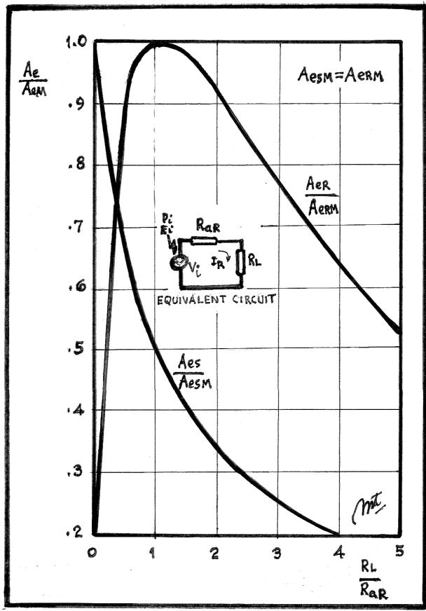 Figure 1. Variation of effective receiving area $A_{eR}$ and effective scattering area $A_{es}$ as a function of the relative terminal resistance $R_L / R_{aR}$, it is assumed identical theoretical antenna perfect resonant and matched. gain for Tx antennas and area for Rx antennas, as well the secondary equation for areas and gain are clearly explained. At a radio link in free space or over ground minimum far field distance is achieved at the maximum Tx antenna radiation. Effective length $L_{eR}$ and factor $AF_{R}$ are inherent in the Rx antenna and independent of distance $r$ and height $H_{R}$. Area and gain are far field parameters or when the wave impedance $Z_{w} = Z_{oo} = 120\pi \simeq 377(\Omega)$. ## III. RADIO LINK BETWEEN TWO IDENTICAL HALF-WAVE DIPOLE ANTENNAS OVER PERFECT GROUND WITH HORIZONTAL POLARIZATION Calculated by a software program (WIPL-D) [6] with the following data, for: $$ \begin{array}{l} \mathrm {f} = 3 0 0 (\mathrm {M H z}), \lambda = 1 (\mathrm {m}), \mathrm {r} = 1 0 0 (\mathrm {m}), \mathrm {H} = 0. 2 3 6 (\mathrm {m}), \\a = 2. 5 (m m), Z _ {a T} = R _ {a T} = 7 1. 4 8 (\Omega), H _ {T} = 2 (m), \\R _ {L} = 7 1. 5 (\Omega), H _ {R} = 1 2. 6 (\mathrm {m}) \\\end{array} $$ Tx antenna power gain $G_{T}$ over perfect ground [2],\[3\]: $G_{T} = 2.15$ (dBi)(free space) + 3 (dB)(image effect) + 3 (dB)(half sphere space radiation) = 8.15 (dBi) (6 dB gain of the same antenna in free space) Rx antenna effective receiving area $A_{eR}$ definition [2],\[3\]: $$ A _ {e R} = W _ {R} / P _ {i} $$ The results obtained are: Tx antenna power gain $G_{TM} = 8.17$ (dBi). Tx antenna maximum power elevation angle $\alpha_{pM} = 7.2^{\circ}$ Tx antenna effective area $A_{eTM} = 0.52(m^2)$ Tx antenna factor $AF_{T71} = 10.0$ (dB/m). Tx antenna factor $AF_{T50} = 11.5$ (dB/m). Rx antenna power gain $G_{R} = 2.17$ (dBi). Rx antenna receiving effective area $A_{eR} = 0.13(m^{2})$ Rx antenna scattering power gain $G_{sM} = 5.20$ (dBi). Rx antenna maximum scattering elevation angle $\alpha_{sM} = 1.1^{\circ}$ Rx antenna scattering effective area $A_{esM} = 0.26(m^2)$ Rx antenna receiving current $I_{R} = 3.1$ E-4 (A). Rx antenna receiving voltage $V_{R} = 2.20$ E-2 (V). Rx antenna receiving power $W_{R} = 6.74$ E-6 (W). Rx antenna factor $AF_{R71} = 16.0(dB / m)$ Rx antenna factor $AF_{R50} = 17.5$ $(dB / m)$ Rx antenna resistance $R_{aR} = 71(\Omega)$ Rx antenna load $R_{L} = 71(\Omega)$ $$ \mathrm {r} ^ {\prime} = \left(r ^ {2} + H _ {R} ^ {2}\right) ^ {1 / 2} = 1 0 0. 7 9 (\mathrm {m}). $$ Maximum incoming power density $P_{iM} = 5.139 \, \text{E-5} \, (W / m^2)$. Receiving power $W_{R} = 6.74$ E-6 (W). Transmission loss or site attenuation $$ A _ {w} = - 5 1. 7 1 (\mathrm {d B}). $$ Free space non dissipative attenuation: $$ A _ {F S} = - 6 2. 0 5 (\mathrm {d B}). $$ Friis secondary equation for parameters in dB: $$ G _ {T} + G _ {R} = 8. 1 7 + 2. 1 7 = 1 0. 3 4 (\mathrm {d B}). $$ $$ A_{w} - A_{FS} = -51.71 - (-62.05) = 10.34 (\mathrm{dB}). $$ Friis power budget fulfilled. Schelkunoff and Friis power reciprocity principle: $$ \begin{array}{l} A _ {e T} / g _ {T} = 0. 0 7 9 \\A _ {e R} / g _ {R} = 0. 0 7 9 \\A _ {e s} / g _ {s} = 0. 0 7 9 \\\end{array} $$ Power reciprocity principle fulfilled. Incident power density or Poynting vector: $$ P _ {i M} = \left(R P _ {y} ^ {2} + R P _ {z} ^ {2}\right) ^ {1 / 2} = 5. 1 3 9 E - 5 \left(W / m ^ {2}\right). $$ Power density elevation angle of the Tx radiation pattern first lobe: $$ \alpha_ {p M} = t g ^ {- 1} \left(R P _ {z} / R P _ {y}\right) = 7.2 ^ {\circ}. $$ Of course, exactly the same elevation angle of the Tx antenna radiation pattern. The maximum power density $P_{iM}$ is travelling along the line of distance $r$ between antennas shown in Figure 2 and at the lower lobe shown in figure 3, fulfilling the Fermat principle. Maximum scattering power density $P_{sM}$ has an elevation angle for the first lobe of $\alpha_{sM} = 1.1^{\circ}$ due to the Rx antenna scattering radiation pattern at the height $H_{R}$. The Rx antenna is a more complex system than the Tx antenna because it 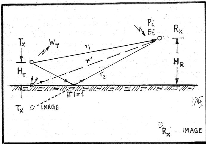 Figure 2. Radio link between two identical half-wave dipole antenna over perfect ground and horizontal polarization. r' distance connects the Tx antenna geometrical center or center phase with the Rx antenna center. Power density $P_{i}$ travels along this line. needs to deliver power to the load $R_{L}$ and, at the same time, scatters EM energy to the surrounding space. These two task have a different radiation patterns, as suggested by Schelkunoff and Friis [3] in his antenna book, but this property was not expanded in their treatise. Rx antenna pattern is practically omnidirectional because it delivers the EM energy on its resistive load but nothing on its image, so it is performing like in free space. This is confirmed by its gain of around 2 (dBi) and almost constant if the Rx antenna is scanned in its height $H_{R}$ [?]. In this case the $G_{R}$ is always close to 2 (dBi) from $H_{R}$ till very close to ground and decreasing slowly to $-\infty(dBi)$ at zero height. The Rx antenna scattering pattern depends, like a Tx antenna, on its height over ground as shown in Figure 3. In this case the Rx antenna height is 12.6 $\lambda$ and it produces 25 lobes between zero and 90 degrees. The Tx antenna at 2 $\lambda$ height produces 4 lobes as shown in Figure 3. It is useful to see the area, gain and factor relation between the Tx and Rx antennas working over perfect ground: $$ \begin{array}{l} A _ {e T} / A _ {e R} = 0. 5 2 / 0. 1 3 = 4. 0 (6 d B). \\g _ {T} / g _ {R} = 6. 5 6 / 1. 6 5 = 3. 9 8 (6 d B). \\A F _ {T 5 0} / A F _ {R 5 0} = 3. 8 0 / 7. 5 8 = 0. 5 (- 6 d B). \\\end{array} $$ For identical resonant and perfectly matched antennas over perfect ground the difference between Tx and Rx antennas of area, gain and factor is 6 dB [10]. ## IV. RX ANTENNA IN SHORT CIRCUIT OVER PERFECT GROUND Following values are considered: $$ \mathrm {f} = 3 0 0 (\mathrm {M H z}), \lambda = 1 (\mathrm {m}), \mathrm {r} = 1 0 0 (\mathrm {m}), \mathrm {H} = 0. 2 3 6 (\mathrm {m}), $$ 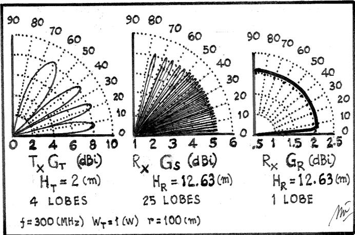 Figure 3. Radio link between two identical half-wave dipole antennas over perfect ground, Tx antenna radiation pattern and Rx antenna receiving and scattering radiation patterns. Tx and Rx antennas are resonant and perfectly matched. $$ \begin{array}{l} \mathrm {a} = 2. 5 (\mathrm {m m}), Z _ {a T} = R _ {a T} = 7 1. 4 8 (\Omega), H _ {T} = 2 (\mathrm {m}), \\\begin{array}{l} \mathrm {a = 2 . 5 (m m) , Z _ {a R} = R _ {a R} = 7 1 . 0 0 (\Omega) , H _ {R} = 1 2 . 6 (m)} \\R _ {L} = 0. 0 (\Omega). \end{array} \\\end{array} $$ Yielding these results by software program (WIPL-D) [6], or: - Tx antenna power gain $G_{TM} = 8.18$ (dBi). - Tx antenna maximum power elevation angle $\alpha_{pM} = 7.2^{\circ}$ - Tx antenna effective area $A_{eTM} = 0.52(m^2)$ - Rx antenna receiving effective area $A_{eR} = 0.0(m^2)$ - Rx antenna scattering power gain $G_{sM} = 8.19$ (dBi). - Rx antenna maximum scattering elevation angle $\alpha_{sM} = 1.1^{\circ}$ - Rx antenna scattering effective area $A_{esM} = 0.52(m^2)$ - Rx antenna receiving current $I_{R} = 6.2$ E-4 (A). - Rx antenna scattering voltage $V_{s} = 4.40$ E-2 (V). - Rx antenna scattering power $W_{s} = 2.73$ E-5 (W). In this case, Tx and Rx antenna have practically the same maximum power gain but different amount of lobes depending on their height over ground. Also, the effective scattering area calculated by the scattering numerical gain $g_{s}$ or by the relation between the scattered power $W_{s}$ and the incoming power density $P_{i}$ yields practically the same result [10]. ## V. RADIO LINK BETWEEN TWO IDENTICAL QUARTER-WAVE MONOPOLE ANTENNAS OVER PERFECT GROUND Tx antenna theoretical power gain $G_{T} = 5.15$ (dBi) Rx antenna theoretical receiving power gain $G_{R} = -0.85$ (dBi). Rx antenna theoretical receiving effective area $$ A _ {e R} = 0. 0 6 5 \lambda^ {2}. $$ Rx antenna theoretical scattering power gain $G_{s} = 2.15$ (dBi). Rx antenna theoretical scattering effective area $A_{es} = 0.13\lambda^2$ Rx antenna theoretical effective height $H_{eR} = 0.159\lambda$ Tx antenna power gain $G_{T}$ over perfect ground [2],[3],\[5\]: $G_{T} = -0.85(\mathrm{dBi})(\lambda /4$ monopole)+ 3 (dB)(image effect)+ 3 (dB)(half sphere space radiation) $= 5.15$ (dB) (6 dB gain over $\lambda /4$ monopole, 3 dB gain over $\lambda /2$ dipole in free space)[10]. Rx antenna effective receiving area $A_{eR}$ definition [2],\[3\]: $A_{eR} = W_{R} / P_{i}$ Software program simulation (WIPL-D) [6], results in: For $\mathrm{f} = 300(\mathrm{MHz})$, $\lambda = 1(\mathrm{m})$, $\mathrm{r} = 100(\mathrm{m})$ $\mathrm{H} = 0.233(\mathrm{m}), \mathrm{a} = 2.5(\mathrm{mm})$ $R_{aT} = R_{aR} = 35.06(\Omega),R_{L} = 50(\Omega),W_{T} = 1(\mathrm{W}).$ Tx antenna power gain $G_{T} = 5.12$ (dBi). Tx antenna effective area $A_{eT} = 0.26(m^{2})$ Tx antenna effective height $H_{eT} = 0.318(m)$ Tx antenna factor $AF_{T50} = 14.65$ (dB/m). Rx antenna receiving power gain $G_{R} = -0.81$ (dBi). Rx antenna receiving effective area $A_{eR} = 0.066(m^{2})$ Rx antenna scattering power gain $G_{s} = 2.11$ (dBi). Rx antenna scattering effective area $A_{es} = 0.13(m^2)$ Rx antenna effective height $H_{eR} = 0.159(m)$ Rx antenna factor $AF_{R50} = 20.57(dB / m)$ Rx antenna received power density $P_{i} = RP_{y} = 2.595$ E-5 $(W / m^{2})$ Rx antenna received power $W_{R} = 1.68$ E-6 (W). Transmission loss or site attenuation $A_{w} = -57.67$ (dB). Free space non dissipative attenuation $A_{FS} = -61.98$ (dB). Secondary Friis equation in dB, results in: $$ G _ {T} + G _ {R} = 5. 1 2 + (- 0. 8 1) = 4. 3 1 (\mathrm {d B}) $$ $$ A_{w} - A_{FS} = -57.67 - (-61.98) = 4.31 (\mathrm{dB}) $$ Friis power budget fulfilled. Schelkunoff and Friis power reciprocity principle \[3\]: $$ \begin{array}{l} A _ {e T} / g _ {T} = 7. 9 6 E - 2 \\A _ {e R} / g _ {R} = 7. 9 6 E - 2 \\A _ {e s} / g _ {s} = 7. 9 6 E - 2 \\\end{array} $$ Monopole antennas, factor, area and gain relations are obtained, as: $$ aF_{T50}/aF_{R50} = 5.40/10.68 = 0.51 (-5.92dB). $$ Relations are very close to 6 dB [10]. The power received $W_{R} = 1.68E - 6(W)$ by this radio link is exactly the same as the radio link between two identical half-wave dipole antennas in free space shown previously. This fulfills the Kenneth Alva Norton Statement [4], or: 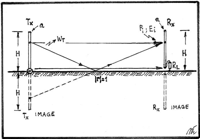 Figure 4. Radio link between two quarter-wave identical monopole antennas over perfect ground. The reflexion effect can be seen as the radiation of the Tx antenna image. Rx antenna image doesn't receive any Tx radiation, because the surface is not transparent. "A radio link between two half-wave dipole antennas in free space delivers the same power $W_{R}$ in the receiving load as a radio link between two quarter wave monopole antennas over perfect ground if the power $W_{T}$ and distance $r$ is the same value". Calculations performed here show that the Norton Statement [4] is perfectly fulfilled if the real or natural antenna gains are used and, therefore, no artificial factors are needed to be introduced to fulfill this Statement, as well as the Friis power budget and the power reciprocity principle [7], [8]. Here no antenna gain were changed in any case like in the papers commented, [7], [8], to force the power budget fulfillment. ## VI. RX QUARTER-WAVE MONOPOLE ANTENNA IN SHORT CIRCUIT Tx antenna theoretical power gain $G_{T} = 5.15$ (dBi) Tx antenna theoretical effective area $A_{eT} = 0.26\lambda^2$ Rx antenna theoretical receiving effective area $A_{eR} = 0.0\lambda^2$ Rx antenna theoretical scattering power gain $G_{s} = 5.15$ (dBi). Rx antenna theoretical scattering effective area $A_{es} = 0.26\lambda^2$ Rx antenna theoretical effective height $H_{eR} = 0.318\lambda$ Results using software program (WIPL-D) \[6\]: Tx antenna power gain $G_{T} = 5.12$ (dBi) Tx antenna effective area $A_{eT} = 0.26m^2$ Tx antenna effective height $H_{eT} = 0.318(m)$. Rx antenna receiving effective area $A_{eR} = 0.0m^2$ Rx antenna scattering power gain $G_{s} = 5.12$ (dBi). Rx antenna scattering effective area $A_{es} = 0.26m^2$ Rx antenna effective height $H_{eR} = 0.318(m)$ ## VII. RADIO LINK BETWEEN TWO SHORT MONOPOLES National Institute of Standards and Technology (NIST) presents in the Technical Note 1347 (January 1991) [12] the calibration of short monopole antennas. These antennas are calibrated to be used as electromagnetic wide band sensors to determine the electromagnetic wave field strength. The procedure is partially theoretical and partially practical. It uses the theoretical equations to find the incoming electric field strength $E_{i}$ over the receiving antenna [11] and the capacity of the receiving antenna $C_{aR}$ [3]. Practically, it measures the input voltage $V_{aT}$ of the transmitting antenna and the input voltage $V_{L}$ of the calibrated receiving field strength meter. These equations are well known and published by books of Jordan [11] and Schelkunoff and Friis [3]. Both monopole antennas are non resonants or adapted at frequencies below $f = 10 \, (MHz)$ because they are of a maximum height of 2.5 (m) for $H_{T}$ and $H_{R}$. Here the simulation of a radio link with two short monopole antennas is calculated and the results are compared to the NIST results. NIST antenna range has a length of 60 (m) and a width of 30 (m) and the surface was metallized in order to get a perfect conductivity of $\sigma \geq 10^{7} \, (S/m)$, that can be considered as practically theoretical (reflexion factor $\Gamma \simeq 1$ ). The transmitting monopole antenna has a radius $a_{1} = 2.5 \, (mm)$ in its base and a radius $a_{2} = 1.3 \, (mm)$ at the top. The receiving monopole antenna has a radius as constant as $a = 0.81 \, (mm)$. Measuring equipments and connexions are installed under ground avoiding interfering the wave fields. NIST is using the classical receiving antenna factor $aF_{aR}$, to be: $$ a F _ {R 5 0} = \frac {E _ {i}}{V _ {R 5 0}} (1 / m) \tag {1} $$ Where: $E_{i}$ (V/m) is the incoming electric field on the receiving monopole antenna. $V_{R50}$ (V) is the measured input voltage on the calibrated receiver with $R_{L} = 50(\Omega)$ impedance. In decibels, results in: $$ A F _ {R 5 0} = 2 0 \log \left(\frac {E _ {i}}{V _ {R 5 0}}\right) (d B / m) \tag {2} $$ For a short monopole antenna $H_{R} \leq 0.1\lambda$ its effective height $H_{eR}$ when the wave impedance is $Z_{w} = Z_{00} = 120\pi \simeq 377(\Omega)$, results in: $$ H _ {e R} = \frac {V _ {i}}{E _ {i}} = \frac {H _ {R}}{2} (m) \tag {3} $$ Where: $V_{i}(\mathrm{V})$ is the induced voltage by the incoming wave in the Thevenin receiving antenna equivalent circuit. $E_{i}$ (V/m) is the incoming electric field on the receiving monopole antenna. Thus: $$ E _ {i} = \frac {V _ {i}}{H _ {e R}} (V / m) \tag {4} $$ From this relation NIST determines the receiving antenna factor $aF_{R50}$ in the $50\Omega$ calibrated receiver, or: $$ a F _ {R 5 0} = \frac {E _ {i}}{V _ {R 5 0}} = \frac {V _ {i}}{V _ {R 5 0} H _ {e R}} = \frac {I _ {R} \left(R _ {L 5 0} + Z _ {a R}\right)}{I _ {R} R _ {L 5 0} H _ {e R}} (1 / m) \tag {5} $$ $I_{R}$ y $R_{L50}$ are common factors in numerator and denominator, results in: $$ a F _ {R 5 0} = \frac {1 + \left(\frac {Z _ {a R}}{R _ {L 5 0}}\right)}{H _ {e R}} (1 / m) \tag {6} $$ $Z_{aR} = R_{aR} + jX_{aR}$ is input impedance of the receiving antenna where the imaginary part $X_{aR}$ is greater than the real part $R_{aR}$, or: $$ Z _ {a R} \simeq - j X _ {a R} (\Omega) \tag {7} $$ With $R_{L50} = 50(\Omega)$ the NIST receiving antenna factor equation, is: $$ a F _ {R 5 0} = \frac {X _ {a R}}{5 0 H _ {e R}} = \frac {X _ {a R}}{2 5 H _ {R}} (1 / m) \tag {8} $$ In decibels, results in: $$ A F _ {R 5 0} = 2 0 \log \left(\frac {X _ {a R}}{2 5 H _ {R}}\right) (d B / m) \tag {9} $$ NIST doesn't determine the receiving antenna input impedance but the receiving antenna capacity using the well known antenna capacity by the equation published by Schelkunoff and Friis [3], or: $$ C _ {a R} = \frac {2 \pi \epsilon_ {0} H}{\ln (H / a) - 1} (F) \tag {10} $$ From this equation the capacitive reactance $X_{aR}$ is obtained: $$ X _ {a R} = \frac {1}{2 \pi f C _ {a R}} (\Omega) \tag {11} $$ Using this procedure, where $R_{aR}$ is negligible, the receiving antenna factor $aF_{R50}$ is reactive and practically imaginary. Here, the simulation is performed as an example at the frequency $f = 3(MHz)$ by means for a radio link between two monopole antennas with the same physical geometry like NIST. The input impedance of both monopoles is obtained by a WIPL-D software [6], or: $$ Z _ {a T} = \left(R _ {a T} + j X _ {a T}\right) = (0. 2 4 - j 2 2 1 7) (\Omega) \tag {12} $$ $$ Z _ {a R} = \left(R _ {a R} + j X _ {a R}\right) = (0. 2 4 - j 2 6 3 7) (\Omega) \tag {13} $$ Transmitted power $W_{T}$ depends from the radiation resistance $R_{aT}$ and the squared current $I_{T}^{2}$ of the transmitting antenna and for a transmitted power $W_{T} = 0.1(W)$, results in: $$ I _ {T} = \left(\frac {W _ {T}}{R _ {a T}}\right) ^ {1 / 2} = \left(\frac {0 . 1}{0 . 2 4}\right) ^ {1 / 2} = 0. 6 4 5 5 (A) \tag {14} $$ The voltage $V_{T}$ on the radiation resistance $R_{aT}$, results in: $$ V _ {T} = \left(I _ {T} R _ {a T}\right) = 0. 6 4 5 5 \cdot 0. 2 4 = 0. 1 5 5 (V) \tag {15} $$ The voltage $V_{Z_{aT}}$ on the transmitting antenna impedance $Z_{aT}$, results in: $$ V _ {Z _ {a T}} = \left(I _ {T} Z _ {a T}\right) (V) \tag {16} $$ $$ V _ {Z _ {a T}} = 0. 6 4 5 5 \cdot (0. 2 4 - j 2 2 1 7) = (0. 1 5 5 - j 1 4 3 1) (V) \tag {17} $$ The voltage is complex with the real part very small compared to the imaginary part. Its module is obtained as: $$ | V _ {Z _ {a T}} | = 1 4 3 1 (V) \tag {18} $$ The voltage $V_{R_g} = 50(\Omega)$ on the generator or amplifier impedance, in order to feed the transmitting antenna, results in: $$ V _ {R _ {g}} = \left(I _ {T} R _ {g}\right) = 0. 6 4 5 5 \cdot 5 0 = 3 2. 3 (V) \tag {19} $$ This way, the voltage $V_{g}$ from the generator or amplifier must be: $$ V _ {g} = \left(V _ {R _ {g}} + V _ {Z _ {a T}}\right) = 1 4 3 1 + 3 2. 3 = 1 4 6 3. 3 (V) \tag {20} $$ The necessary power $W_{g}$ to produce the transmitting power $W_{T} = 0.1(W)$, result in: $$ W _ {g} = \left(V _ {g} I _ {T}\right) = 1 4 6 3. 3 \cdot 0. 6 4 5 5 = 9 4 4. 5 6 (W) \tag {21} $$ It is very important to see the low efficiency of the power supply when a transmitting antenna is very reactive and with no impedance matching. Almost 1 KW to radiate $100\mathrm{mW}$. For this reason NIST uses a power amplifier to feed the transmitting short monopole. But it is the only way to feed a wide band short antenna at frequencies lower than 10 MHz. In simulation the voltage using WIPL-D to feed the transmitting antenna is $|V_{Z_aT}| = 1431(V)$ and transmitting gain, field strength and power density obtained at the distance $r = 30(m)$, are: $$ G_{T} = 4.77 (dBi) $$ $$ g _ {T} = 2. 9 9 $$ $$ E _ {i} = 8. 9 3 6 E - 2 (V / m) $$ $$ E _ {z} = (- 7. 2 6 9 E - 2 - j 5. 1 9 8 E - 2) (V / m) $$ $$ H _ {i} = 3. 0 0 7 E - 4 (A / m) $$ $$ H _ {x} = (- 2. 1 6 5 E - 4 - j 2. 0 8 7 E - 4) (A / m) $$ $$ P _ {i} = 2. 6 8 7 E - 5 (V / m) $$ $$ P _ {y} = (2. 6 5 9 E - 5 - j 3. 9 1 3 E - 6) \left(W / m ^ {2}\right) $$ The wave impedance is obtained as: $$ | Z _ {w} | = 2 9 7. 1 7 (\Omega), Z _ {w} = (2 9 4 - j 4 3) (\Omega) $$ At the distance of $r = 30(m)$ the far field is not really achieved because the wave impedance is not $Z_{w} = Z_{00} = 377(\Omega)$ but a lower value with a little reactance value. However, the simulation is done according to the field modules. Open circuit voltage $V_{i}$ for an effective height $H_{eR} = 1.25(m)$, results in: $$ V _ {i} = \left(H _ {e R} E _ {i}\right) = 1. 2 5 \cdot 8. 9 3 6 E - 2 = 0. 1 1 1 7 (V) \tag {22} $$ Current module $I_R$ in the receiving antenna equivalent Thevenin circuit for $R_L = 50(\Omega)$, results in: $$ I _ {R} = \left(\frac {V _ {i}}{R _ {L} + X _ {a R}}\right) (A) \tag {23} $$ $$ I _ {R} = \left(\frac {0 . 1 1 1 7}{5 0 + 2 6 3 7}\right) = 4. 1 6 E - 5 (A) \tag {24} $$ The receiving voltage $V_{R50}$, is obtained as: $$ V _ {R 5 0} = (5 0 \cdot I _ {R}) = 5 0 \cdot 4. 1 6 E - 5 = 2. 0 8 E - 3 (V) \tag {25} $$ Receiving antenna factor $aF_{R50}$, results in: $$ a F _ {R 5 0} = \left(\frac {E _ {i}}{V _ {R 5 0}}\right) = \left(\frac {8 . 9 3 6 E - 2}{2 . 0 8 E - 3}\right) = 4 2. 9 6 (1 / m) \tag {26} $$ The antenna factor $AF_{R50}$ in decibels is: $$ A F _ {R 5 0} = (2 0 \log a F _ {R 5 0}) = 3 2. 6 6 (d B / m) \tag {27} $$ This is a pure imaginary antenna factor. If an antenna factor could be real, complex or imaginary, the area of the receiving antenna could get the same characteristics because the power on the load impedance $R_{L50}$ could be complex. Using the classical equation: $$ A _ {e R} = \left(\frac {W _ {R}}{P _ {i}}\right) (1 / m) \tag {28} $$ The power at the calibrated receiver input, results in: $$ W _ {R 5 0} = \left(R _ {L} \cdot I _ {R} ^ {2}\right) = 5 0 \cdot (4. 1 6 E - 5) ^ {2} = 8. 6 5 E - 8 (W) \tag {29} $$ And the effective area, results in: $$ A _ {e R} = \left(\frac {W _ {R}}{P _ {i}}\right) (m ^ {2}) \tag {30} $$ $$ A _ {e R} = \left(\frac {8 . 6 5 E - 8}{2 . 6 8 7 E - 5}\right) = 3. 2 2 E - 3 \left(m ^ {2}\right) \tag {31} $$ Numerical receiving antenna gain, according to Schelkunoff and Friis, results in: $$ g _ {R} = \left(\frac {4 \pi}{\lambda^ {2}}\right) A _ {e R} = \frac {4 \pi}{1 0 0 ^ {2}} (3. 2 2 E - 3) = 4. 0 5 E - 6 \tag {32} $$ The receiving antenna gain $G_{R}$ in decibels, results in: $$ G _ {R} = 1 0 \log \left(\frac {4 \pi}{\lambda^ {2}}\right) A _ {e R} = - 5 3. 9 3 (d B i) \tag {33} $$ The transmission loss $a_{w}$ in the radio link is obtained, as: $$ a _ {w} = \left(\frac {W _ {R}}{W _ {T}}\right) \tag {34} $$ $$ a _ {w} = \left(\frac {8 . 6 5 E - 8}{0 . 1}\right) = 8. 6 5 E - 7 \tag {35} $$ The power transmission loss or site attenuation $A_{w}$ in decibels, results in: $$ A _ {w} = 1 0 \log a _ {w} = - 6 0. 6 3 (d B) \tag {36} $$ Free space $A_{FS}$ in decibels, results in: $$ A _ {F S} = 1 0 \log \left(\frac {\lambda}{4 \pi r}\right) ^ {2} = - 1 1. 5 3 (d B) \tag {37} $$ Gain and losses relationship, according to Schelkunoff and Friis [3], results in: $$ G _ {T} + G _ {R} = 4. 7 7 + (- 5 3. 9 3) = - 4 9. 1 6 (d B) \tag {38} $$ $$ A _ {w} - A _ {F S} = - 6 0. 6 3 - (- 1 1. 5 3) = - 4 9. 1 0 (d B) \tag {39} $$ Friis radio link power budget is fullfilled. Scattering gain in dBi is calculated by software WIPL-D, as: $$ G _ {s} = - 1 8. 3 3 (d B i) \tag {40} $$ Numerical scattered gain $g_{s}$, results in: $$ g _ {s} = 1. 4 7 E - 2 \tag {41} $$ Scattering area is obtained by the isotropic radiator area $A_{eo}$ and the numerical scattering gain $g_{s}$, as: $$ A _ {e s} = \left(\frac {\lambda^ {2}}{4 \pi}\right) g _ {s} = 1 1. 7 0 (m ^ {2}) \tag {42} $$ Transmitting antenna effective area $A_{eT}$, is obtained this way, knowing its numerical gain $g_{T}$, or: $$ A _ {e T} = \left(\frac {\lambda^ {2}}{4 \pi}\right) g _ {T} = 2 3 7 9. 3 7 (m ^ {2}) \tag {43} $$ Relation between areas and gain, according to Schelkunoff and Friis [3] are: $$ \left(\frac {A _ {e T}}{g _ {T}}\right) = \left(\frac {2 3 7 9 . 3 7}{2 . 9 9}\right) = 7 9 5. 8 \tag {44} $$ $$ \left(\frac {A _ {e s}}{g _ {s}}\right) = \left(\frac {1 1 . 7 0}{1 . 4 7 E - 2}\right) = 7 9 5. 9 \tag {45} $$ $$ \left(\frac {A _ {e R}}{g _ {R}}\right) = \left(\frac {3 . 2 2 E - 3}{4 . 0 5 E - 6}\right) = 7 9 5. 1 \tag {46} $$ All cases are giving practically the same results. At this example of $f = 3(MHz)$ in the radio link with a transmitted power $W_{T} = 100(mW)$ the received voltage is $V_{R50} = 2.08E - 3(V)$ or $V_{R50} = -26.82(dBV)$ or in power $W_{R50} = 8.65E - 8(W)$ or $W_{R50} = -70.63(dBW)$ and the antenna factor $AF_{R50} = 32.66(dB / m)$. According to the reciprocity principle (Schelkunoff and Friis) is possible to calculate the transmitting antenna factor $aF_{T50}$ [10], to be: $$ a F _ {T} = \left(\frac {1}{\lambda}\right) \left(\frac {4 \pi Z _ {w}}{R _ {L} g _ {T}}\right) = 4. 9 9 E - 2 (1 / m) \tag {47} $$ in decibels: $$ A F _ {T} = 2 0 \log \left(\frac {1}{\lambda}\right) \left(\frac {4 \pi Z _ {w}}{R _ {L} g _ {T}}\right) = - 1 3. 0 2 (d B / m) \tag {48} $$ For this example the relationship between factors, areas and gain for the monopole antennas for $H_{T}, H_{R} = 2.5(m)$, results in: $$ \left(\frac {a F _ {R 5 0}}{a F _ {T 5 0}}\right) = \left(\frac {4 2 . 9 6}{4 . 9 9 E - 2}\right) = 8 6 0. 9 2 (5 8. 7 d B) \tag {49} $$ $$ \left(\frac {A _ {e T}}{A _ {e R}}\right) = \left(\frac {2 3 8 7 . 3 2}{3 . 2 2 E - 3}\right) = 7 4 1 4 0 3. 7 3 (5 8. 7 d B) \tag {50} $$ $$ \left(\frac {g _ {T}}{g _ {R}}\right) = \left(\frac {2 . 9 9}{4 . 0 5 E - 6}\right) = 7 3 8 2 7 1. 6 (5 8. 7 d B) \tag {51} $$ These relationship are giving the same result in dB. This means the radio link was calculated accurately. An important Table I RESULTS OF ANTENNA FACTOR $AF_{R50}$ FOR SHORT MONOPOLE ANTENNAS AS A FUNCTION OF FREQUENCY IN MHz. COLUMNS 2,3 Y 4 CALCULATED BY NIST, COLUMNS 5,6 Y 7 CALCULATED FOR A RADIO LINK WITH A TRADICIONAL PROCEDURE SHOWN PREVIOUSLY FOR $f = 3(MHz)$. <table><tr><td>f</td><td>\({X}_{aR} \)</td><td>\(a{F}_{50} \)</td><td>\(A{F}_{R50} \)</td><td>\({Z}_{aR} \)</td><td>\(a{F}_{R50} \)</td><td>\(A{F}_{R50} \)</td></tr><tr><td>MHz</td><td>(Ω)</td><td>(1/m)</td><td>(dB/m)</td><td>(Ω)</td><td>(1/m)</td><td>(dB/m)</td></tr><tr><td>1.0</td><td>8038</td><td>128.61</td><td>42.19</td><td>0.027-j7969</td><td>127.39</td><td>42.10</td></tr><tr><td>1.5</td><td>5359</td><td>85.74</td><td>38.66</td><td>0.060-j5306</td><td>84.75</td><td>38.56</td></tr><tr><td>2.0</td><td>4019</td><td>64.30</td><td>36.16</td><td>0.107-j3972</td><td>63.29</td><td>36.03</td></tr><tr><td>3.0</td><td>2679</td><td>42.87</td><td>32.64</td><td>0.241-j2637</td><td>42.96</td><td>32.66</td></tr><tr><td>5.0</td><td>1607</td><td>25.71</td><td>28.20</td><td>0.668-j1555</td><td>24.88</td><td>27.92</td></tr><tr><td>7.5</td><td>1072</td><td>17.15</td><td>24.69</td><td>1.500-j1004</td><td>16.13</td><td>24.15</td></tr><tr><td>10.0</td><td>804</td><td>12.86</td><td>22.19</td><td>2.660-j 718</td><td>11.56</td><td>21.26</td></tr></table> thing to know is, in the case of the short antennas, the difference between identical antennas characteristics over ground are extremely different and not only 6 dB like in the case of resonant and perfectly matched identical antennas [10]. Here is shown that the equation 7 in the Standard IEEE-ANSI C63.5-2004 cannot be used because the factors, area and gain are not the same for identical antennas when they are operating over perfect ground. Different procedure must be used. NIST (Technical Note 1347) [12] have not calculate all the parameters obtained here in order to know the behavior of both antennas and their characteristics. Doing the same simulation for other frequencies the results are presented in Table I. In this table it can be shown that the results obtained are practically identical to that obtained by NIST. ## VIII. TRANSMITTING ANTENNA FACTOR DEFINITION Transmitting antenna factor $aF_{T}$ was not defined as the receiving antenna factor $aF_{R}$, or: $$ a F _ {R} = \frac {E _ {i}}{V _ {R}} = \left(\frac {P _ {i} Z _ {o o}}{W _ {R} R _ {L}}\right) ^ {1 / 2} = \left(\frac {Z _ {o o}}{A _ {e R} R _ {L}}\right) ^ {1 / 2} (1 / m) \tag {52} $$ However, is possible to determine the transmitting antenna factor by means of the Power Reciprocity Principle according to Schelkunoff and Friis [3]. According to the Receiving antenna factor definition: $$ a F _ {R} = \frac {E _ {i}}{V _ {R}} = \left(\frac {P _ {i} Z _ {o o}}{W _ {R} R _ {L}}\right) ^ {1 / 2} = \left(\frac {Z _ {o o}}{A _ {e R} R _ {L}}\right) ^ {1 / 2} (1 / m) \tag {53} $$ It is possible to determine the relation between the receiving numerical antenna factor $aF_{R}$ to the receiving antenna effective area $A_{eR}$, in the far field when the wave impedance $Z_{w} = Z_{oo} = 120\pi \simeq 377(\Omega)$, or: $$ \boxed {a F _ {R} = \left(\frac {Z _ {o o}}{A _ {e R} R _ {L}}\right) ^ {1 / 2} (1 / m)} \tag {54} $$ Receiving antenna effective area, in the far field, results in: $$ A _ {e R} = \frac {\lambda^ {2} g _ {R}}{4 \pi} (m ^ {2}) \tag {55} $$ This way, is possible to determine the relation between the receiving numerical antenna factor $aF_{R}$ to the receiving antenna numerical gain $g_{R}$ in the far field, or: $$ \boxed {a F _ {R} = \frac {1}{\lambda} \left(\frac {4 \pi Z _ {o o}}{g _ {R} R _ {L}}\right) ^ {1 / 2} (1 / m)} \tag {56} $$ Power reciprocity principle presented by Schelkunoff and Friis [3], is expressed as: $$ \frac {A _ {e T}}{g _ {T}} = \frac {A _ {e R}}{g _ {R}} \tag {57} $$ Or: $$ \frac {A _ {e T}}{A _ {e R}} = \frac {g _ {T}}{g _ {R}} = \left(\frac {a F _ {R}}{a F _ {T}}\right) ^ {2} \tag {58} $$ Transmitting antenna factor results in: $$ a F _ {T} = a F _ {R} \left(\frac {g _ {R}}{g _ {T}}\right) ^ {1 / 2} (1 / m) \tag {59} $$ $$ a F _ {T} = \left(\frac {Z _ {o o}}{A _ {e R} R _ {L}} \frac {g _ {R}}{g _ {T}}\right) ^ {1 / 2} (1 / m) \tag {60} $$ $$ \boxed {a F _ {T} = \frac {1}{\lambda} \left(\frac {4 \pi Z _ {o o}}{g _ {T} R _ {L}}\right) ^ {1 / 2} (1 / m)} \tag {61} $$ This equation is exactly the same as for the receiving antenna factor but instead of the numerical gain $g_{R}$ for the transmitting antenna the numerical gain $g_{T}$ must be used. At the same time, it is seen that these equations are that indicated by the Federal Communication Commission (F.C.C.) to calculate the antenna factors if the space intrinsic impedance $Z_{oo} = 120\pi = 377(\Omega)$, wavelength in (m) and a load resistance $R_{L} = 50(\Omega)$ must be used. In dB, it results in: $$ \boxed {A F _ {R} = 1 9. 7 7 - 2 0 \log \lambda - 1 0 \log g _ {R} (d B / m)} \tag {62} $$ For a receiving antenna. $$ \boxed {A F _ {T} = 1 9. 7 7 - 2 0 \log \lambda - 1 0 \log g _ {T} (d B / m)} \tag {63} $$ For a transmitting antenna. As a function of space intrinsic impedance $Z_{oo} = 120\pi = 377(\Omega)$, frequency in $MHz$ and a load resistance $R_{L} = 50(\Omega)$, results in: $$ \boxed {A F _ {R} = - 2 9. 7 8 + 2 0 \log f _ {M H z} - 1 0 \log g _ {R} (d B / m)} \tag {64} $$ For a receiving antenna. $$ \boxed {A F _ {T} = - 2 9. 7 8 + 2 0 \log f _ {M H z} - 1 0 \log g _ {T} (d B / m)} \tag {65} $$ For a transmitting antenna. These equations are valid for a radio link in free space or over a perfect ground using the corresponding gain obtained in the indicated environment. Over perfect ground the maximum gain obtained for a theoretical half wave dipole antenna is $G_{T} = 8.15(dBi)$ or very close to this value in an actual environment and $G_{R} = 2.15(dBi)$ for a receiving half wave antenna at practically any height over perfect ground [10]. Around $R_{aT} = R_{aR} = 73(\Omega)$ is obtained for the radiation resistance of a resonant dipole. $(R_{aT} = R_{aR} = 70 \text{to} 73(\Omega))$ in practical thin dipoles. In the case of a theoretical quarter wave monopoles over perfect ground maximum gain for a transmitting antenna is $G_{T} = 5.15(dBi)$ at zero elevation angle and $G_{R} = -0.85(dBi)$ for the receiving antenna [10]. Around $R_{aT} = R_{aR} = 34$ to $36(\Omega)$ of a radiation resistance is obtained in resonance for thin monopoles. In conclusion it was demonstrated that the antenna parameters in a radio link over perfect ground have a difference of 6 dB in favor of the transmitting antenna for perfect resonant and matched antennas, in the maximum radiation [10]. This is valid for any identical antenna used in the radio link. For not perfectly matched antennas this difference is even larger, as demonstrated previously, in this paper. ## IX. CONCLUSIONS The comments that have been presented here show that a radio link, in free space or over perfect ground, using any kind of antennas, can be verified using the Friis equation and achieve the power budget and the power reciprocity principle in order to be sure that the radio link is working properly. No artificial factors are needed to obtain this result if the proper antenna gain is used [7],[8]. In the case of a quarter wave monopole antenna its gain over a perfect absorbing surface has a theoretical gain of $G_{T} = -0.85(dBi)$ (theoretically a real monopole). Over a perfect reflective surface its image increases its length to a half-wave (a real dipole), that in free space has a gain of $G_{T} = 2.15(dBi)$. For this reason, a called monopole over perfect ground needs to only cover the half spherical space over ground and this increases its gain additionally by 3 (dB) achieving the well known gain of $G_{T} = 5.15(dBi)$ and maintaining its radiation resistance in resonance $R_{aT} \simeq 36(\Omega)$, because mutual effects are not available. Dr Wolff made a perfect explanation of a Tx quarter-wave monopole antenna characteristics showing that its effective area is twice the area of a half-wave dipole antenna in free space and its logical gain $G_{T} = 5.15[dBi]$. However, he said nothing about the characteristics of Rx quarter wave monopole antenna whose effective area is half the area of a half-wave dipole in free space and its logical receiving gain $G_{R} = -0.85[dBi]$. This means 3 (dB) larger gain of a half-wave dipole antenna in free space who needs to cover all the spherical area with its radiated energy. This problem was solved in the thirthie's in the golden AM BC era. In the receiving case its effective area is half that of the half-wave dipole in free space and from it, according to Schelkunoff and Friis, its receiving gain is $G_{R} = -0.85(dBi)$, a true monopole without image. At the same time, any receiving antennas in the receiving role work like in free space, because no transmitting energy is arriving at its image if the surface is not transparent. Thus, it works practically independent of its height over ground and of its distance from the transmitting one. Of course, in scattering the Rx antenna works practically like a Tx antenna and its reradiation or scattering depends on its height over ground and with its image assistance. This also, is verified in the case of the monopole-dipole radio link where the gain of the monopole is $G_{T} = 5.15$ (dBi) and the dipole over ground has a receiving gain, as was determined previously, of $G_{R} = 2.15$ (dbi), practically constant like in free space. In all case analyzed, the power budget and the power reciprocity principle are fulfilled perfectly well without changing the natural antenna gains and showing the perfect radio link work. The Tx antenna gain, well known since the thirties, add 6 db at its gain compared to the gain of the same antenna in free space. This depends of the image effect like in the monopole antenna case. These results have been corroborated experimentally in the RF spectrum in MF, HF, VHF and UHF confirming that the Rx antenna in the receiving role works without the image effect or like in free space. It was determined that in the short monopole antenna case the difference between identical antennas in transmission and reception is extremely greater than in the case of resonant and well matched antennas and not only 6 dB. Here it is shown that over perfect or natural ground identical antennas have always different characteristics as factor, area and gain. It is also important to know that: the antenna area $A_{eT}A_{eR}$ and gain $g_{T}g_{R}$ are parameters valid accurately in far field $r \gg \lambda$ when the wave impedance $Z_{w}$ is really $Z_{00} = 120\pi$ and the effective length $L_{eR}$ or height $H_{eR}$ and the antenna factor $aF_{T}aF_{R}$ is a parameter inherent of the antenna, for this reason they are practically constant from the distance or height over ground. However, these parameters can be related between them in the far field. ### ACKNOWLEDGEMENT Assistance to prepare these comments by Walter Gustavo Fano, Lucas Gonzalez and Ramiro Alonso are very much appreciated. Special thanks to the late good friend and colleague Ermi Roos of Miami Fl who consulted me about this problem found in BC Monopole measurements about twenty year ago. Also to Dr. Gary Thiele for our long time discussions.

Generating HTML Viewer...

References

11 Cites in Article
H Friis (1946). A Note on a Simple Transmission Formula.
J Kraus (1950). Unknown Title.
S Schelkunoff,H Friis (1952). Antennas: Theory and Practice. Sergei A. Schelkunoff and Harald T. Friis. New York: Wiley; London: Chapman & Hall, 1952. 639 pp. $10.00.
Kenneth Norton (1953). Transmission Loss in Radio Propagation.
E Wolff (1966). Antenna Analysis.
B Kolundzija,J Ognjanovic,T Sarkar (1999). WIPL-D Software Electromagnetic Modeling of Composite Metallic and Dielectric Structures.
J Logan,J Rockway (1997). Dipole and Monopole Antenna Gain and Effective Area for Communication Formulas. Naval Command, Control and Ocean Surveillance Center.
G Thiele (2019). Friis Transmission over Ground Plane.
A Ben,Munk (2003). Finite Antenna Arrays and FSS.
Valentino Trainotti (2018). Antenna characteristics over perfect ground.
Edward Jordan,C Andrews (1950). Electromagnetic Waves and Radiating Systems.
No ethics committee approval was required for this article type.
Data Availability
Not applicable for this article.
How to Cite This Article
Valentino Trainotti. 2026. \u201cComments on Friis Transmission over a Ground Plane\u201d. Global Journal of Computer Science and Technology - H: Information & Technology GJCST-H Volume 22 (GJCST Volume 22 Issue H2).
Explore published articles in an immersive Augmented Reality environment. Our platform converts research papers into interactive 3D books, allowing readers to view and interact with content using AR and VR compatible devices.
Your published article is automatically converted into a realistic 3D book. Flip through pages and read research papers in a more engaging and interactive format.
Our website is actively being updated, and changes may occur frequently. Please clear your browser cache if needed. For feedback or error reporting, please email [email protected]
Thank you for connecting with us. We will respond to you shortly.