## I. INTRODUCTION The aim of image compression is the transmission of images over communication channels with limited bandwidth. It is essential and important in multimedia applications such as Mobile, Bluetooth, Internet browsing, computer to computer communication etc. The image compression applications also include bio-medical, satellite, aerial surveillance, reconnaissance, multimedia communication and ground water survey etc. The most commonly used image compression techniques are Joint Photography Expert Author p: Electronics and Communication Engineering, Vaagdevi College of Engineering, Warangal, India. Group (JPEG), JPEG-2000, TIF and PNG, the first two techniques use Discrete Cosine Transform (DCT) and Discrete Wavelet Transform (DWT) respectively. Among all the image compression techniques, DWT based image compression has shown better compression ratio and image quality. Bing et al proposed fast convolution algorithm (FCA) for DWT calculation by observing the symmetric properties of filters and hence the computational complexity is reduced. Compared with ordinary convolution, the FCA decreases the multiplication operations by nearly one half. Converted into real programming, it sped up the DWT and IDWT by at least $12\%$ and $55\%$, respectively [1]. In addition to increasing the computational speed by $81.35\%$, the coefficients performed much better than the reported coefficients in literature. To reduce computational complexity further, wavelets were progressed on resized, cropped, resized-average and cropped-average images [2]. However, symmetric and orthogonal filters design is critical, so multi-wavelets were introduced which offer supplementary filters with desired properties [3]. These filter coefficients are further partition into blocks of unique size and based on the coefficient variance a bit assignment table was computed and blocks of individual class were coded using bit assignment table [4]. In addition, fast orientation prediction-based discrete wavelet transform (DWT) is also used to improve coding performance and to reduce computational complexity by designing a new orientation map and orientation prediction model for high-spatial-resolution remote sensing images [5]. Farid et al have modified JPEG by Baseline Sequential Coding which is based on near optimum transfer and entropy coding and trade-off between reconstructed image quality and compression ratio is controlled by quantizers [6]. Individually the wavelet transform (WT) based compression method is able to provide a compression ratio of about 20-30, which is not adequate for many practical situations. So there is a need of hybrid approach which would offer higher compression ratio than the WT alone keeping the quality of reproduced image identical in both cases. The hybrid combinations for medical image compression such as DWT and Artificial Neural Network (ANN) [7], discrete wavelet transform and discrete cosine transform (DCT) [8], hybridization of discrete wavelet transform (DWT), log polar mapping (LPM) and phase correlation [9], hybridization of empirical wavelet transform (EWT) along with discrete wavelet transform has been used for compression of the ECG signals [10]. The hybrid wavelet combines the properties of existing orthogonal transforms and these wavelets have unique properties that they can be generated for various sizes and types by using different component transforms and varying the number of components at each level of resolution [11], Hybridization of wavelet transforms and vector quantization (VQ) for medical ultrasound (US) images. In this hybridization, the sub-band DWT coefficients are grouped into clusters with the help vector quantization [12]. On other side, image compression can also be performed with the non-transformed techniques such as vector quantization and image thresholding. Kaur et al proposed image compression that models the wavelet coefficients by generalized Gaussian distribution (GGD) and suitable sub bands are selected with suitable quantizer. In order to increase the performance of quantizer, threshold is chosen adaptively to zero-out the unimportant wavelet coefficients in the detail sub bands before quantization [13]. Kaveh et al proposed a novel image compression technique which is based on adaptive thresholding in wavelet domain using particle swarm optimization (PSO). In multi-level thresholding, thresholds are optimized without transforming the image and thresholds are optimized with computational intelligence techniques (swarm evolutionary and metaheuristic optimization techniques). It is observed that thresholding image compression is better with wavelet transform than without transform. Optimal thresholds are optimized with PSO algorithm. Thresholded image is further coded with an arithmetic coding and results proved better compared to Set partitioning in hierarchical trees (SPIHT), JPEG, JPEG2000 and Chrysafis in peak signal to noise ratio and reconstructed image quality [14] In this paper, for the first time the application of optimization techniques for selection of the optimal thresholds is explored which reduces the distortion between the input image and reconstructed image. The aim of this work is the selections of optimal thresholds which zero-out the insignificant discrete wavelet transform coefficients in all sub-bands. The performance of different optimization techniques and their optimal variable parameters are compared. The performance measures are peak signal to noise ratio and reconstructed image quality. This paper is organized in five sections including the introduction. In section 2 proposed framework of adaptive thresholding for Image compression is discussed. The proposed method of Thresholding using Bat algorithm is presented along with the procedure in section 3. The results and discussions are given in section 4. Finally the conclusion is given in section 5. ## II. PROPOSED FRAMEWORK OF ADAPTIVE THRESHOLDING FOR IMAGE COMPRESSION ### a) 2-D Discrete Wavelet Transform In 1970's images are decomposed with Discrete Cosine Transform (DCT) in which most of the energy is concentrated in DC coefficients, that helps high compression with baring considerable artifact effect. Recently Discrete Wavelet Transform (DWT) positioned the image compression to a subsequent level. Unlike DCT, the DWT provides both spatial and frequency information of the image. The DWT decomposes the image into four coefficients; approximation (low-low frequency (LL)), horizontal (low-high frequency (LH)), vertical (high-low frequency (HL)) and diagonal (high-high frequency (HH)) coefficients. These coefficients are obtained with parallel combination of low pass filter and high pass filter and down samplers as shown in Fig. 1. 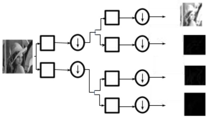 Figure 1: Wavelet Decomposition spread their values near around to particular values, which help for good thresholding/clustering results better image compression as shown in Fig. 2d. For next level (2nd level) of decomposition the LL band is decomposed into four coefficients as like in first level of decomposition so achieved a LL2, LH2, HL2 and HH2. This process is repeated for next level (3rd level) of decomposition so achieved a ten sub-images in total. Fig. 3 shows a 3rd level decomposition of Lena image. Like in JPEG-2000, the wavelet used in our work for decomposition is bi-orthogonal wavelet because of its design is simple and option to build symmetric wavelet functions. For the sake of fidelity of reconstructed image quality and comparison with the published work, three level and five level decomposition is applied, the same can be applied to more than five decomposition levels for a high degree of compression at the cost of time. In the proposed method, optimization technique spent much time for thresholding of approximation coefficients and less time for remaining, because the reconstructed image quality depends predominantly on approximation coefficients.  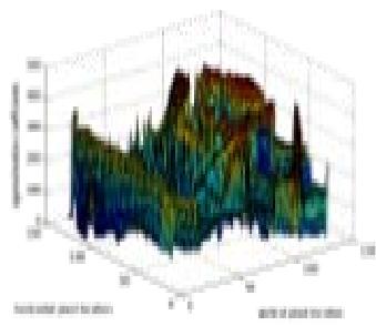Fig. 2 shows the three dimensional view of approximation, horizontal, vertical and diagonal coefficients of a Lena image. 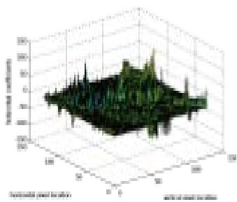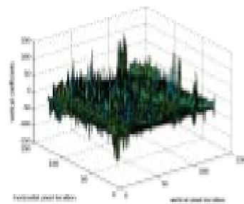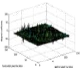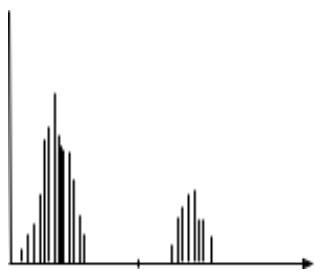It is observed that approximation coefficients carry much information about the input image as compared to other coefficients whereas all horizontal, vertical and diagonal coefficients    Figure 2: Three dimensional View of Approximation, Horizontal, Vertical and Diagonal Coefficients of a Lena Image  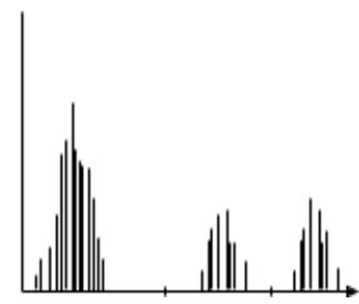 Figure 3: Image Histogram of an Image F(X,Y) ### b) Thresholding Image thresholding is the process of extracting the objects in a scene from the background that helps for analysis and interpretation of the image. Selection of threshold is moderately simple in case where histogram of the image has a deep valley represents background and sharp edges represent objects, but due to the multimodality of the histograms of many images, selections of a threshold are a difficult task. Thresholding can be classified into two types: Global Thresholding and Level Dependent/Local Thresholding. In global thresholding-image compre ssion is obtained using a single threshold value for all the decomposition levels, whilst in level dependent thresholding-image compression is achieved using different threshold values for different decomposition level. The energy levels being different in decomposition levels of the image are the main criterion for the application of the level thresholding method in this paper. The histogram of an image $f(x, y)$ that is composed of several light objects on a dark background may represent two dominate modes as shown in Fig. 3 The two modes can be separated by selecting an appropriate threshold $T$ and hence the object information can be extracted from the background. If the image is comprised of several objects then different thresholds are required to separate the object classes as shown in Fig. 3. If $f(x,y)$ lies between $T_{1}$ and $T_{2}$ the object may be classified as belonging to one object class. If $f(x,y)$ is greater than $T_{2}$ the object belongs to a second class. If $f(x,y)$ is less than or equal to $T_{1}$ then object belongs to the background. As compared to single level thresholding, this process of threshold selection to obtain the object class is usually less reliable. Thresholding may be viewed as an operation that tests against a given function of the form $$ T = T [ x, y, p (x, y), f (x, y) ] \tag {1} $$ Where, $f(x,y)$ is the gray level of point $(x,y)$, $p(x,y)$ is some local property of the input i.e. the average gray level of a neighbourhood around $(x,y)$. The thresholded image is given by $$ \mathrm{c} (\mathrm{x}, \mathrm{y}) = \left\{ \begin{array}{c c c} c (\mathrm{x}, \mathrm{y}) & if & \mathrm{c} (\mathrm{x}, \mathrm{y}) > \mathrm{T} \\ T & if & \mathrm{c} (\mathrm{x}, \mathrm{y}) \leq \mathrm{T} \end{array} \right. 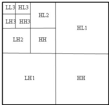\tag{2} $$  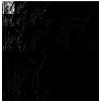 Figure 4: 3-level DWT of Lena Image The objects and background are represented by pixels labelled 1 (or any other convenient threshold value $T$ ) and pixels labelled 0 respectively. The threshold is termed as global threshold if $T$ depends only on $f(x,y)$ and local threshold if $T$ depends on $f(x,y)$ and $p(x,y)$. The threshold is called dynamic, if $T$ depends on the spatial coordinates $(x,y)$, in addition to the above cases. For instance, priory if certain information regarding the nature of the object is known a local threshold may be utilised, whereas a dynamic thresholding may be used if object illumination is non-uniform. Thresholding technique find many real time applications like data, image and video compression, image recognition, pattern recognition, image understanding and communication. In this proposed method of thresholding in wavelet domain, different thresholds are assigned for different sub-bands. In 3 level decomposition, there are 10 sub-bands i.e LL3, LH3, HL3, HH3, LH2, HL2, HH2, LH1, HL1 and HH1as shown in Fig. 4. Among all ten sub-bands LL3, LH3, HL3 and HH3 possess very high energy and hence these are assigned to four individual thresholds (i.e. $T1$, $T2$, $T3$ and $T4$ ) and play a very significant role in the reconstructed image quality at the decoder section. As more number of thresholds are made use for the image reconstruction it increases the computational time of the optimization techniques, but the quality of the image is emphasized more than the computational time. The remaining sub-bands (LH2, HL2 and HH2) and (LH1, HL1 and HH1) have the less energy level as compared to sub-bands LL3, LH3, HL3 and HH3. Therefore the sub-bands LH2, HL2, HH2 are assigned to single threshold $T5$ and the LH1, HL1 and HH1 are assigned to another single threshold $T6$. Also the same procedure is adapted for five level decomposition of the image. It consists of sixteen subbands in total, out of which four low frequency subbands are assigned to four individual thresholds ( $T1$ to $T4$ ) and the remaining twelve sub-bands are partitioned into four groups which consists of three sub-bands each and these four groups are assigned to four thresholds ( $T5$ to $T8$ ). In this work much prominence is given to low frequency sub-bands as mostly reconstructed image quality depends on the low frequency sub-bands and more over these sub-bands carry very high energy of the input image. After the initialization of the thresholds is completed, these are optimized with various optimization techniques by maximizing/minimizing the objective function or fitness function as defined in Eq (3). The main aim of optimization techniques is to find a better threshold that reduces the distortion between original image and reconstructed image. The optimization technique that produces thresholds with less distortion is treated as a superior optimization technique. In this work, objective function/fitness function that is used for the selection of optimal thresholds is a combination of the entropy and PSNR values in order to obtain high compression ratio and better reconstructed image quality. Here entropy is assumed as compression ratio. Therefore, the fitness function is defined as following [14]: $$ f i t n e s s = a \times e n t r o p y + \frac {b}{P S N R} \tag {3} $$ Where $a$ and $b$ are adjustable arbitrary user defined parameters and are varied as per the requirement of user to obtain the required level of compression ratio and distortion respectively. In general the maximum and minimum values of the population in a optimization technique is a constant value whereas in this context maximum and minimum values are lies between maximum and minimum value of the respective sub-band image coefficients because of the selection of different thresholds for different sub-bands, during the computational procedure of the algorithm. The optimal thresholds are obtained successfully with the application of the proposed Bat algorithm. If the coefficients of the corresponding sub-band is less than the corresponding threshold then replace the coefficients with the respective threshold else coefficients remains the same. Let $T$ represents a threshold value for a particular subband then its corresponding coefficients follows the Eq. (4) to generate thresholded image. $$ \mathrm{c} (\mathrm{x}, \mathrm{y}) = \left\{ \begin{array}{c c c} c (\mathrm{x}, \mathrm{y}) & if & \mathrm{c} (\mathrm{x}, \mathrm{y}) > \mathrm{T} \\ T & if & \mathrm{c} (\mathrm{x}, \mathrm{y}) \leq \mathrm{T} \end{array} \right. \tag{4} $$ Thresholding image is further coded by run-length coding (RLE) followed by Huffman coding. Run-length Coding is a lossless coding that aims to reduce the amount of data needed for storage and transmission and represents consecutive runs of the same value in the data as the value, followed by the count or vice versa. RLE reduces the thresholded image to just two pixel values when all the pixel values in the thresholded image are unique and if the pixel values of threshold image are not unique then it doubles the size of the original image. Therefore, RLE is applied only in cases where the expect runs of the same value are of importance. Huffman coding is a losses variable length coding which is best fit for compressing the outcome of RLE. As the RLE produces repetitive outcomes, the probability of a repeated outcome is defined as the desired outcome, which can be obtained by integrating RLE and Huffman coding techniques. Repeated outcomes are represented by fewer bits and higher bits are used to represent infrequent outcomes. The performance of Huffman coding purely depends on the effective development of Huffman tree with minimum weighted path length. The time complexity of Huffman coding is $O(N \log_2 N)$. ## III. THRESHOLDING USING BAT ALGORITHM PSO generates efficient thresholds but undergoes instability in convergence when practical velocity is high [15]. Firefly algorithm (FA) was developed to generate near global thresholds but it experiences a problem when no such significant brighter fireflies in the search space [15]. So a Bat algorithm (BA) is developed that gives a global threshold with minimum number of iterations. It is a nature inspired Metaheuristic algorithm developed by YANG in 2010 [16]. Bat algorithm works with the three assumptions: 1. All bats use echolocation to sense distance, and they also 'know' the difference between food/prey and background barriers in some magical way; 2. Bats fly randomly with velocity $v_{i}$ at position $x_{i}$ with a fixed frequency $Q_{\min}$, varying wavelength and loudness $A_{0}$ to search for prey. They can automatically adjust the wavelength (or frequency) of their emitted pulses and adjust the rate of pulse emission $r \in [0,1]$, depending on the proximity of their target; 3. Although the loudness can vary in many ways, we assume that the loudness varies from a large (positive) $A_{0}$ to a minimum constant value $A_{\min}$. Intensification (local search/local optimum) of the algorithm is attaining with pulse rate and diversification (global search/local optimum) is attaining with loudness parameter. Here thresholds are assumed as Bats. The detailed Bat algorithm is as follows: Step 1: (Initialize the bat & parameters): Initialize the number of thresholds $(n)$ and randomly select the threshold values i.e., $X_{i}$, $(i = 1,2,3,\dots$, n), loudness (A), velocity (V), pulse rate (R), minimum frequency (Qmin) and maximum frequency (Qmax). Step 2: (Find the best threshold): Calculate the fitness of all thresholds using Eq. (3), and the best fitness threshold is the Xbest. Step 3: (Automatic zooming of threshold towards Xbest): Each threshold is zoomed as per Eq. (7) by adjusting frequency in Eq. (5) and velocities in Eq. (6). Frequency update: $$ Q_{i}(t+1)=Q\max(t)+(Q\min(t)-Q\max(t))^{*}\boldsymbol{\theta} $$ Where $\pmb{\theta}$ is random number [0 to 1] Velocity update: $$ v _ {i} (t + 1) = v _ {i} (t) + \left(X _ {i} - X b e s t\right) ^ {*} Q _ {j} (t + 1) \tag {6} $$ $$ X _ {i} (t + 1) = X _ {i} (t) + v _ {i} (t + 1) \tag {7} $$ Step 4: (Selection of step size of random walks): If generated random number is greater than pulse rate $R$ then move the threshold around the selected best threshold based on Eq. (8). $$ X _ {i} (t + 1) = X \text{best} (t) + w * R _ {i} \tag{8} $$ Where $R_{i} =$ random numbers, $w =$ step size for random walk Step 5: (Generate a new threshold): Generate a random number, if it is less than loudness and new threshold fitness is better than the old threshold, accept the new threshold. Step 6: Rank the bats and find the current best Xbest. Step 7: Repeat step (2) to (6) until maximum iterations. ## IV. RESULTS AND DISCUSSIONS The proposed method of image compression in discrete wavelet domain using bat algorithm based optimal thresholding has been executed in MATLAB environment with a laptop of HP Probook 4430s, Intel core i5 processor, 2GB random access memory (RAM). The performance of the algorithm is tested for the readily available standard images obtained from the link www(imageprocessingplace.com. Six popular images which are extensively used for compression test images like Barbara, Cameraman, Gold Hill, Jet Plane, Lena, and Peppers are selected to test the performance of the proposed algorithm. The experimental results of published methods for the above said images are available in the literature. For the simulation of PSO algorithm, the Trelea type-2 PSO toolbox is used. The same parameters as in paper [14] are selected for PSO as well as to QPSO such as number of particles, maximum number of epochs, distortion and compression ratio parameter (a, b). Similarly for firefly algorithm a particular value to tuning parameters is selected where its performance is better in compression ratio and reconstructed image quality. The parameter values are finalized after the implementation of firefly algorithm to the problem stated. The parameters which are set for tuning of firefly algorithm are alpha $(\alpha) = 0.01$, beta minimum $(\beta_0) = 1$, gamma $(\gamma) = 1$. The maxima of maximum of average PSNR obtained from the repeated experimental results for loudness and pulse rate with respect to PSNR as shown in Fig. 5, is chosen as the Bat algorithm parameter value for simulating the Lena image. From experimental shown in Fig. 5, it can be observed that Loudness = 0.3 and Pulse rate = 0.1, and the same parameters values are used for later experiments. The remaining parameters: frequency Qmin = 0.3, Qmax = 0.9 and step-size of random walks = 0.36 is selected randomly. The performance measuring parameter for evaluation of effectiveness and efficiency of the proposed method is Peak Signal to Noise Ratio (PSNR) and objective function/fitness function. The equation for fitness function is as given in Eq (3) and PSNR value of original signal $f(X,Y)$ and reconstructed image $g(X,Y)$ is calculated using Eq (9) $$ P S N R = 1 0 \times 1 0 \log \left(\frac {2 5 5 ^ {2}}{M S E}\right) (\mathrm {d B}) \tag {9} $$ Where Mean Square Error (MSE) is given as $$ M S E = \frac {1}{M \times N} \sum_ {X} ^ {M} \sum_ {Y} ^ {N} \left\{f (\mathrm {X}, \mathrm {Y}) - \mathrm {g} (\mathrm {X}, \mathrm {Y}) \right\} ^ {2} \tag {10} $$ Where $M \times N$ is size of image, $X$ and $Y$ represents the pixel value of original and reconstructed/decompressed images. In our experiment we have taken $N = M$ a square image. $f(X,Y)$ is an original image and $g(X,Y)$ reconstructed image of size 512 by 512. The performance of the proposed method of image compression in frequency domain for the six images is compared with the other techniques such as PSO, QPSO and FA.  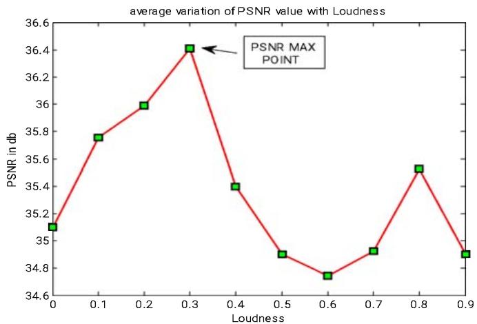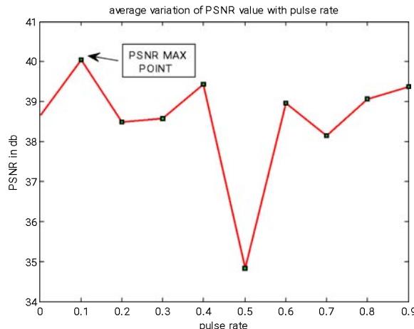(a)  (b) Figure 5: Average PSNR of Lena Image being Performed 5 times for Selection of Parameter (A) Loudness (B) Pulse Rate Table 1-6 shows PSNR of the proposed method and other methods for six tested images. From tables it is observed that the PSNR achieved with the proposed method is better than the PSO, QPSO and FA. As five level and three level decomposition are used so for the sake of comparison [14], a three level and five level decomposition with appropriate (a, b) parameters is also chosen. Parameters (a, b) are adjusted according to the user requirements to maintain trade-off between compression ratio and reconstructed image quality as both objectives cannot be achieved at the same time. Table 1-6 shows the (a, b) values to achieve corresponding bits per pixels for six images. The major drawback with the PSO and firefly is that large number of tuning parameters and improper parameter tuning causes performance degradation of the PSO and FA, whereas in bat algorithm only two tuning parameters are enough, so effect of tuning parameters on BA is much smaller compared to PSO and FA. The bat algorithm optimization process combines the advantages of simulated annealing and particle swarm optimization process and with the concept of frequency tuning, the PSNR values which indicates the quality of the image is superior to PSO and FA as well as harmony search. With suitable simplifications PSO and harmony search becomes the special cases of Bat algorithm. In addition the bat algorithm possesses the benefit of automatic zooming that is accompanied by the automatic switch from explorative moves to local intensive exploitation, which results in fast convergence rate as compared to other techniques Table 1: PSNR Comparison for Barbara Image at Different Bit Per Pixel (BPP) <table><tr><td>BPP</td><td>a,b</td><td>a,b</td><td colspan="2">PSO</td><td colspan="2">QPSO</td><td colspan="2">FA</td><td colspan="2">BA</td></tr><tr><td></td><td>3-level</td><td>5-level</td><td>3-level</td><td>5-level</td><td>3-level</td><td>5-level</td><td>3-level</td><td>5-level</td><td>3-level</td><td>5-level</td></tr><tr><td>0.125</td><td>(11,1)</td><td>(11,1)</td><td>25.60</td><td>25.72</td><td>25.63</td><td>25.82</td><td>25.71</td><td>25.92</td><td>26.05</td><td>26.32</td></tr><tr><td>0.250</td><td>(10,1)</td><td>(9,1)</td><td>28.32</td><td>28.42</td><td>28.39</td><td>28.47</td><td>28.43</td><td>28.64</td><td>28.83</td><td>28.93</td></tr><tr><td>0.500</td><td>(8,1)</td><td>(8,2)</td><td>32.15</td><td>32.34</td><td>32.55</td><td>32.71</td><td>32.78</td><td>32.98</td><td>32.96</td><td>33.23</td></tr><tr><td>1.000</td><td>(4,1)</td><td>(4,1)</td><td>37.10</td><td>37.12</td><td>37.15</td><td>37.31</td><td>37.39</td><td>37.64</td><td>37.52</td><td>37.83</td></tr><tr><td>1.250</td><td>(2,1)</td><td>(2,1)</td><td>39.98</td><td>40.04</td><td>40.08</td><td>40.24</td><td>40.34</td><td>40.53</td><td>40.44</td><td>40.87</td></tr></table> Table 2: PSNR Comparison for Gold Hill Image at Different Bit Per Pixel (BPP) <table><tr><td>BPP</td><td colspan="2">(a, b)</td><td colspan="2">PSO</td><td colspan="2">QPSO</td><td colspan="2">FA</td><td colspan="2">BA</td></tr><tr><td></td><td>3-level</td><td>5-level</td><td>3-level</td><td>5-level</td><td>3-level</td><td>5-level</td><td>3-level</td><td>5-level</td><td>3-level</td><td>5-level</td></tr><tr><td>0.125</td><td>(7,1)</td><td>(4,1)</td><td>29.12</td><td>29.19</td><td>29.28</td><td>29.42</td><td>29.41</td><td>29.62</td><td>29.44</td><td>29.67</td></tr><tr><td>0.250</td><td>(5,1)</td><td>(3,2)</td><td>31.28</td><td>31.43</td><td>31.39</td><td>31.51</td><td>31.58</td><td>31.64</td><td>31.61</td><td>31.77</td></tr><tr><td>0.500</td><td>(3,1)</td><td>(2,3)</td><td>33.81</td><td>33.93</td><td>33.92</td><td>34.13</td><td>33.99</td><td>34.41</td><td>34.05</td><td>34.51</td></tr><tr><td>1.000</td><td>(2,2)</td><td>(1,5)</td><td>37.27</td><td>37.40</td><td>37.31</td><td>37.58</td><td>37.55</td><td>37.75</td><td>37.65</td><td>37.90</td></tr><tr><td>1.250</td><td>(1,5)</td><td>(1,7)</td><td>41.75</td><td>41.90</td><td>41.82</td><td>41.95</td><td>41.96</td><td>42.11</td><td>42.01</td><td>42.32</td></tr></table> Table 3: PSNR Comparison for Lena Image at Different Bit Per Pixel (BPP) <table><tr><td>BPP</td><td colspan="2">(a, b)</td><td colspan="2">PSO</td><td colspan="2">QPSO</td><td colspan="2">FA</td><td colspan="2">BA</td></tr><tr><td></td><td>3-level</td><td>5-level</td><td>3-level</td><td>5-level</td><td>3-level</td><td>5-level</td><td>3-level</td><td>5-level</td><td>3-level</td><td>5-level</td></tr><tr><td>0.125</td><td>(15,1)</td><td>(15,1)</td><td>30.82</td><td>30.98</td><td>30.91</td><td>31.08</td><td>31.11</td><td>31.15</td><td>31.23</td><td>31.43</td></tr><tr><td>0.250</td><td>(11,1)</td><td>(10,1)</td><td>35.17</td><td>35.26</td><td>35.21</td><td>35.32</td><td>35.34</td><td>35.46</td><td>35.45</td><td>35.68</td></tr><tr><td>0.500</td><td>(7,1)</td><td>(7,1)</td><td>37.91</td><td>38.23</td><td>37.98</td><td>38.28</td><td>38.18</td><td>38.55</td><td>38.35</td><td>38.70</td></tr><tr><td>1.000</td><td>(4,1)</td><td>(4,2)</td><td>40.94</td><td>41.42</td><td>40.97</td><td>41.53</td><td>41.27</td><td>41.67</td><td>41.33</td><td>41.71</td></tr><tr><td>1.250</td><td>(2,1)</td><td>(2,3)</td><td>42.15</td><td>42.31</td><td>42.19</td><td>42.37</td><td>42.30</td><td>42.46</td><td>42.47</td><td>42.62</td></tr></table> Table 4: PSNR Comparison for Cameraman Image at Different Bit Per Pixel (BPP) <table><tr><td>BPP</td><td colspan="2">(a, b)</td><td colspan="2">PSO</td><td colspan="2">QPSO</td><td colspan="2">FA</td><td colspan="2">BA</td></tr><tr><td></td><td>3-level</td><td>5-level</td><td>3-level</td><td>5-level</td><td>3-level</td><td>5-level</td><td>3-level</td><td>5-level</td><td>3-level</td><td>5-level</td></tr><tr><td>0.125</td><td>(18,1)</td><td>(16,1)</td><td>26.17</td><td>26.53</td><td>26.21</td><td>26.60</td><td>26.37</td><td>26.71</td><td>26.43</td><td>26.74</td></tr><tr><td>0.250</td><td>(12,1)</td><td>(11,1)</td><td>30.05</td><td>30.10</td><td>30.09</td><td>30.15</td><td>30.17</td><td>30.41</td><td>30.27</td><td>30.56</td></tr><tr><td>0.500</td><td>(10,1)</td><td>(10,2)</td><td>33.46</td><td>33.52</td><td>33.51</td><td>33.63</td><td>33.55</td><td>33.69</td><td>33.58</td><td>33.73</td></tr><tr><td>1.000</td><td>(3,1)</td><td>(3,2)</td><td>38.02</td><td>38.13</td><td>38.09</td><td>38.19</td><td>38.21</td><td>38.37</td><td>38.33</td><td>38.39</td></tr><tr><td>1.250</td><td>(1,1)</td><td>(1,1)</td><td>40.11</td><td>40.23</td><td>40.13</td><td>40.28</td><td>40.33</td><td>40.32</td><td>40.43</td><td>40.51</td></tr></table> Table 5: PSNR Comparison for Jetplan Image at Different Bit Per Pixel (BPP) <table><tr><th>BPP</th><th colspan="2">(a,b)</th><th colspan="2">PSO</th><th colspan="2">QPSO</th><th colspan="2">FA</th><th colspan="2">BA</th></tr><tr><th></th><th>3-level</th><th>5-level</th><th>3-level</th><th>5-level</th><th>3-level</th><th>5-level</th><th>3-level</th><th>5-level</th><th>3-level</th><th>5-level</th></tr><tr><th>0.125</th><th>(12,1)</th><th>(12,1)</th><th>27.98</th><th>28.23</th><th>27.98</th><th>28.28</th><th>28.04</th><th>28.33</th><th>28.11</th><th>28.39</th></tr><tr><th>0.250</th><th>(10,1)</th><th>(10,1)</th><th>31.38</th><th>31.65</th><th>31.41</th><th>31.69</th><th>31.51</th><th>31.72</th><th>31.57</th><th>31.80</th></tr><tr><th>0.500</th><th>(8,1)</th><th>(7,1)</th><th>34.12</th><th>34.32</th><th>34.18</th><th>34.32</th><th>34.25</th><th>34.45</th><th>34.37</th><th>34.53</th></tr><tr><th>1.000</th><th>(3,1)</th><th>(3,1)</th><th>38.89</th><th>38.97</th><th>38.92</th><th>39.05</th><th>38.99</th><th>39.25</th><th>39.15</th><th>39.44</th></tr><tr><th>1.250</th><th>(1,1)</th><th>(1,1)</th><th>41.16</th><th>41.24</th><th>41.18</th><th>41.30</th><th>41.25</th><th>41.41</th><th>41.46</th><th>41.63</th></tr></table> Table 6: PSNR Comparison for Pepper Image at Different Bit Per Pixel (BPP) <table><tr><th>BPP</th><th colspan="2">(a,b)</th><th colspan="2">PSO</th><th colspan="2">QPSO</th><th colspan="2">FA</th><th colspan="2">BA</th></tr><tr><th></th><th>3-level</th><th>5-level</th><th>3-level</th><th>5-level</th><th>3-level</th><th>5-level</th><th>3-level</th><th>5-level</th><th>3-level</th><th>5-level</th></tr><tr><th>0.125</th><th>(10,1)</th><th>(9,1)</th><th>34.81</th><th>34.98</th><th>34.82</th><th>35.01</th><th>34.89</th><th>35.16</th><th>34.90</th><th>35.21</th></tr><tr><th>0.250</th><th>(5,1)</th><th>(4,1)</th><th>37.58</th><th>37.82</th><th>37.63</th><th>37.89</th><th>37.69</th><th>37.98</th><th>37.73</th><th>38.18</th></tr><tr><th>0.500</th><th>(1,1)</th><th>(1,1)</th><th>39.75</th><th>39.92</th><th>39.84</th><th>40.12</th><th>39.92</th><th>40.27</th><th>40.12</th><th>40.44</th></tr><tr><th>1.000</th><th>(3,1)</th><th>(1,4)</th><th>42.92</th><th>43.21</th><th>42.98</th><th>43.33</th><th>43.04</th><th>43.46</th><th>43.26</th><th>43.61</th></tr><tr><th>1.250</th><th>(1,5)</th><th>(1,5)</th><th>43.10</th><th>43.42</th><th>43.19</th><th>43.43</th><th>43.29</th><th>43.52</th><th>43.38</th><th>43.74</th></tr></table> ## V. CONCLUSIONS This paper presents a novel approach to obtain image compression in discrete wavelet domain by optimizing threshold values using bat algorithm for the first time. The coefficients obtained by applying discrete wavelet transform for the image to be compressed are classified into different groups by making use of the optimal thresholds, these optimal thresholds are obtained using bat algorithm, keeping a balance between the quality of the reconstructed image and compression ratio. The proposed technique is simple and adaptive in nature as individual thresholds are assigned to high energy sub-bands individually and for rest of the sub-bands a common threshold are assigned. The successful thresholded image is further coded with Runlenght coding followed by Hauffman coding. It is observed that for multilevel thresholding bat algorithm produces superior PSNR values, good quality of the reconstructed image with less convergence time as compared to PSO and firefly as the later techniques are unstable if the particle velocity is maximum and no brighter firefly in the search space respectively. The algorithm convergence time is further improved by the fine adjustment of the pulse emission and loudness parameters and time delay between pulse emission and the echo. ### ACKNOWLEDGMENT This work is supported by Ministry of Human Resource and Management (MHRD), Govt. of India and Management of GMR Institute of Technology, Rajam, Andhrapredesh.

Generating HTML Viewer...

References

16 Cites in Article
Bing Fei Wu,Chorng Yann Su (1999). A fast convolution algorithm for biorthogonal wavelet image compression.
K Shanavaz,P Mythili (2013). Faster techniques to evolve wavelet coefficients for better fingerprint image compression.
Miete P R Deshmukh,A A Ghatol,Fiete (2002). Multiwavelet and Image Compression.
V Singh (1999). Discrete wavelet transform based image compression.
Libao Zhang,Bingchang Qiu (2013). Fast orientation prediction-based discrete wavelet transform for remote sensing image compression.
G Panda,S Meher (2006). An Efficient Hybrid Image Compression Scheme using DWT and ANN Techniques.
S Singh,V Kumar,H Verma (2007). DWT–DCT hybrid scheme for medical image compression.
Ahmed Louchene,Ammar Dahmani (2013). WATERMARKING METHOD RESILIENT TO RST AND COMPRESSION BASED ON DWT, LPM AND PHASE CORRELATION.
Rakesh Kumar,Indu Saini (2014). Empirical Wavelet Transform Based ECG Signal Compression.
B Hemant,Kekre,K Tanuja,Rekha Sarode,Vig (2015). A new multi-resolution hybrid wavelet for analysis and image compression.
L Kaur,R Chauhan,S Saxena (2006). Wavelet based compression of medical ultrasound images using vector quantization.
L Kaur,R Chauhan,S Saxena (2006). Joint thresholding and quantizer selection for compression of medical ultrasound images in the wavelet domain.
Kaveh Ahmadi,Ahmad Javaid,Ezzatollah Salari (2015). An efficient compression scheme based on adaptive thresholding in wavelet domain using particle swarm optimization.
K Chiranjeevi,J Umaranjan (2016). Fast vector quantization using a Bat algorithm for image compression.
Yang (2010). A New Metaheuristic Bat-Inspired Algorithm, in: Nature Inspired Cooperative Strategies for Optimization (NISCO 2010).
No ethics committee approval was required for this article type.
Data Availability
Not applicable for this article.
How to Cite This Article
Chiru K. 2026. \u201cNovel Wavelet Domain Based Adaptive Thresholding using Bat Algorithm for Image Compression\u201d. Global Journal of Computer Science and Technology - F: Graphics & Vision GJCST-F Volume 23 (GJCST Volume 23 Issue F1).
Explore published articles in an immersive Augmented Reality environment. Our platform converts research papers into interactive 3D books, allowing readers to view and interact with content using AR and VR compatible devices.
Your published article is automatically converted into a realistic 3D book. Flip through pages and read research papers in a more engaging and interactive format.
Our website is actively being updated, and changes may occur frequently. Please clear your browser cache if needed. For feedback or error reporting, please email [email protected]
Thank you for connecting with us. We will respond to you shortly.