## I. INTRODUCTION Due to their compactness and their ability to transmit high loads at high speeds, gears are widely used in automotive and aerospace applications through speed reducers, power transmissions in wind turbines, etc. In gear drives energy efficiency improving may require reducing power losses. Power losses in gears (gearboxes, reducers, etc.) can be grouped into two categories: power losses depending on the transmitted load (friction at the contact areas between the teeth and friction in the bearings, etc.) and those independent of the transmitted load (losses due to the trapping of the lubricant, the ventilation of the mobiles, etc.). Several researchers have been interested in load-dependent losses and enough models exist. The oil trapping in the inter-tooth space and the ventilation of the spindles are the two main sources of power dissipation in the case of losses independent of the loads. Very few studies and models exist on the loss of power by lubricant trapping and by consequent on the modeling of lubricant leakage surfaces. The vast majority of studies concerning the modeling of lubricant trapping in the inter-tooth space are empirical, numerical, and semi-analytical and based on approximations and estimations. The first experimental studies on this subject permitted to make a difference between load-dependent and load-independent losses. Devin R. and Hilty B.[1], made experimental investigations of load-independent losses caused by planetary gear sets and conclude that for high speeds $(\geq 6000~\mathrm{rpm})$ the losses independent of the load become the major contributor. These experimental works allowed to develop and validate empirical, numerical and semi-analytical models. Using NASA research center test rig, Anderson and al. [2], Krantz [3], Rohn and Handschuh [4] have developed several empirical formulas. Empirical formulations for the particular case of trapping losses in gears are based on the gears geometric parameters and include those of Terekhov [5], Wolfan Mauz [6], Butsch M. [7] and Maurer J. [8]. The empirical models developed provided global formulas for the estimation of pressing torque or power loss. It is necessary to point out that these formulas are only valid for external gearing and remain linked to the sensitivity and precision of the equipment used for the tests. Generally they are of very low precision with quite important deviations. As an example we can quote the model of Mauz[6], which indicates an uncertainty between 5 and $15\%$ if the resisting torque is higher than $5\mathrm{Nm}$ and an uncertainty up to $50\%$ for lower torque values. It is therefore necessary to set up another quite precise model. Many researchers have developed numerical models to understand the behavior of inter-tooth spaces during movement in order to estimate the power lost by trapping. Pechersky and Wittbrodt [9] used an approximation of the tooth profile expression to calculate the leakage surfaces. Diab Y. and al [10-11] have numerically evaluated the radial leakage surfaces (considered here as minimum distances between the tip corner of the gear and the profile) and they obtained the axial leakage surfaces by numerical integration. Abdelilah Lasri and al [12-14] used a numerical approximation to evaluate the radial surfaces (considered here as the minimum distance between the tooth profiles) and they obtained the axial leakage surfaces by numerical integration. David C. Talbot [15] calculates the power lost by trapping in planetary gears by discretizing in time and space the Conservation of Mass, Momentum and Energy equations. The leakage surfaces are obtained by numerical approximation through the surfaces meshing. Seetharaman and Kahraman [16] were inspired by the work of Pechersky and Wittbrodt [9] to establish a semi-analytical formulation for calculating leakage surfaces. However, several approximations are made there, namely a Taylor approximation of order 1 of the involute profile equation, the cancellation of certain portions of the surface, the use of approximate values of certain distances, etc. From the vectors ray approach, Massimo Rundo[17] established an analytical formula for trapped volume in crescent pumps. It is necessary to note that in this approach the length variation of the vector ray for an infinitesimal rotation is neglected. In addition, this formula is limited only to the portion where teeth profiles are in contact. For an efficient contribution to the power losses by the lubricant trapping of as well as the wear of the elements with a view to improve the energy performances in gears transmissions, it is essential to completely lift the veil on the inter-tooth zone during meshing. From the work of Seetharaman and Kahraman [16], we will establish a purely analytical model of the evolution of the radial and axial leakage surfaces as a function of the angle of rotation in a spur gear. This work has as particularity the use of the exact expression of the tooth profile in the calculations and the authenticity of the analytical expressions of the developed surfaces. This work is divided into three main parts. The first part is devoted to the modeling of the tooth profile and the associated parametric equations. The second part deals with the calculations of the leakage surfaces from the tooth profile equations, with the radial leakage surface being considered as the minimum distance between the tooth profiles. The last part focuses on the results interpretation and the model validation. The model validation consists of a superposition of our results with those of A. Lasri and al [13] and Diab and al [10]. ## II. MATERIAL ### a) Trapping Phenomenon The lubricant used in gear transmissions to reduce corrosion, friction, cool the elements, etc., is trapped in the inter-tooth space during movement and becomes the seat of energy losses. Lubricant trapping is the jamming of the lubricant in the inter-tooth space during the meshing phase. The fraction of lubricant trapped in the inter-tooth space (in yellow in figure 1) is expelled under pressure radially toward the neighbouring pockets and or axially toward the outside of the gear during this phenomenon. The opposite phenomenon is reproduced during the unmeshing phase. The geometry of the inter-tooth space relates to the type of tooth (straight, helical, hypoid, etc.) which constitutes the gear's wheels. In the particular case of spur gears, the axial leakage area remains constant over the tooth width. However, in the case of helical gear, the axial leakage area is variable over the tooth width. 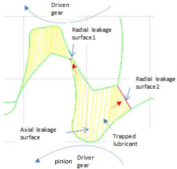 Figure 1: Inter-tooth space and trapped lubricant ### b) Evolution of Radial and Axial Leakage Surfaces The radial and axial leakage surfaces vary according to the angle of rotation. The further away from the initial position, the surfaces increase. Here, the initial position is the meeting point between the two pitch circles. The Figure 2 below illustrates the behavior of the leakage surfaces as a function of the angle of rotation from a) to h). 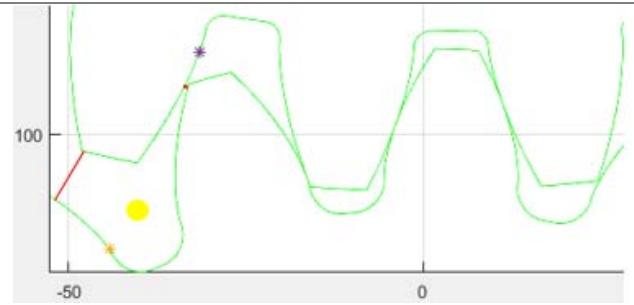 a) Location $\phi_{1} = 0,4287$ rad 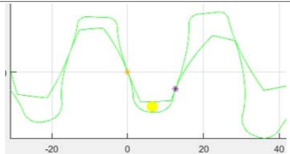 e) Location $\phi_{1} = -\beta_{1} = -0,0713$ rad 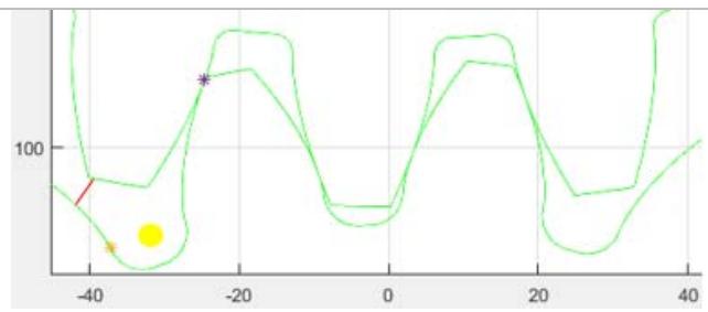 b) Location $\phi_{1} = 0,3558$ rad 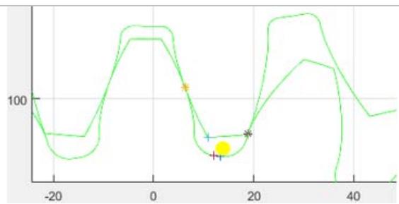 f) Location $\phi_{1} = -1493$ rad 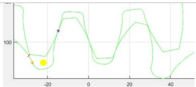 c) Location $\phi_{1} = 0,2392$ rad 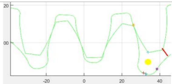 g) Location $\phi_{1} = -0,3658$ rad 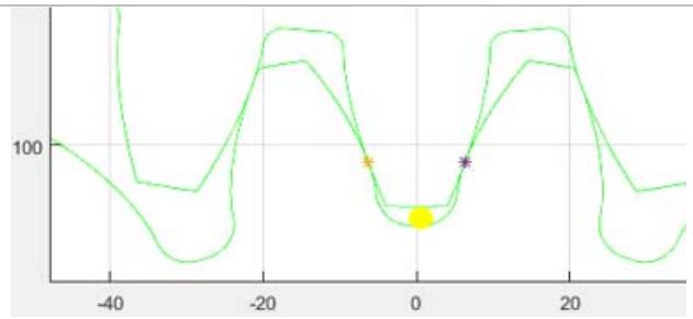 d) Location $\phi_1 = 0$ rad 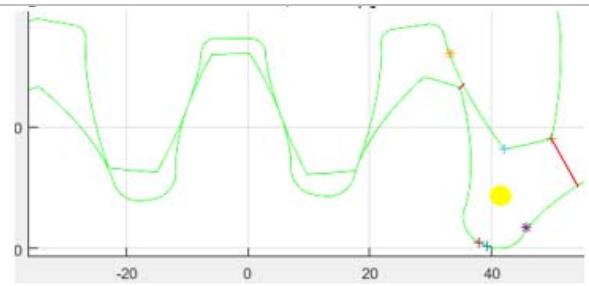 h) Location $\phi_{1} = -0,4458$ rad Figure 2: Evolution of the leakage surfaces as a function of the rotation angle ### c) Coordinate System Linked to Gears The pinion (driver) is associated to a fixed reference $(O_{f},x_{f},y_{f},z_{f})$ and mobile reference $(O_{1},x_{1},y_{1},z_{1})$, which revolves around $(O_{f},z_{f})$ by an angle $\phi_{1}$. Similarly, the gear (driven) is associated to fixed reference $(O_{p},x_{p},y_{p},z_{p})$ and mobile reference $(O_{2},x_{2},y_{2},z_{2})$, which revolves around $(O_{p},z_{p})$ by an angle $\phi_{2}$. Such as $\phi_{2} = -(\rho_{1} / \rho_{2})\phi_{1} = -(r_{1} / r_{2})\phi_{1} = -(r_{s1} / r_{s2})\phi_{1}$. Figure 3 below illustrates all these different references. 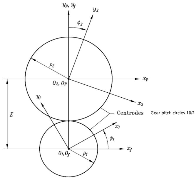 Figure 3: Tracking of gear system In our calculations, the initial position is the position where the tooth profiles of the driving and driven gears meet at point I (the contact point between the pitch circles). ### d) Geometry of a Spur Gear Tooth The tooth shapes of spur gears are relative to the number of teeth. Generally, for a tooth, there will be the involute zone and the circular zone. Figure 4 below shows the detailed geometry of a 25-tooth gear. 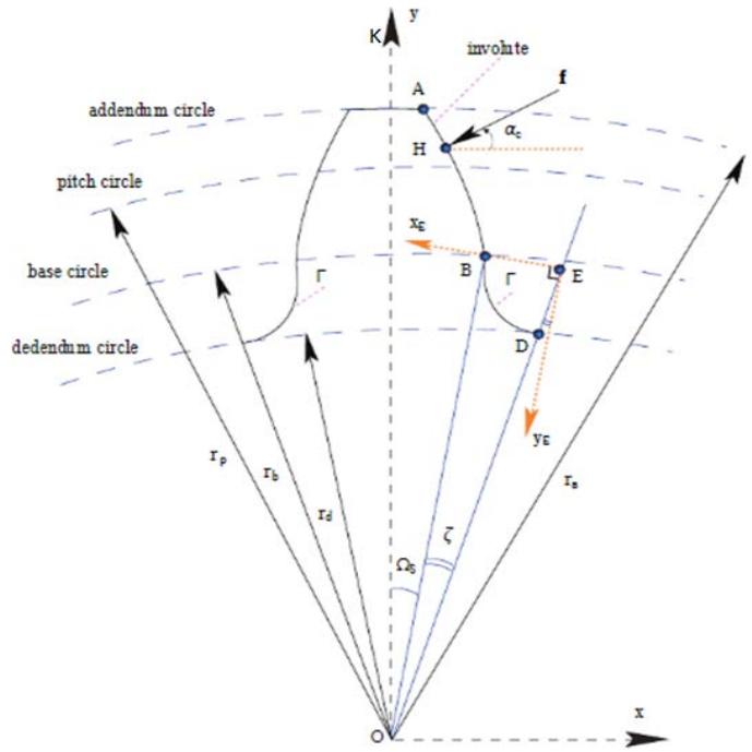 Figure 4: Geometry of an external spur gear ### e) Leakage Surface and Border Points at a given Location In a specific interval of the rotation angle, the profiles of the teeth meet, and consequently the radial leakage surfaces remain zero. Figure 5 below is a particular case. On this figure, C1 and C2 are the two contact points of the tooth profiles. 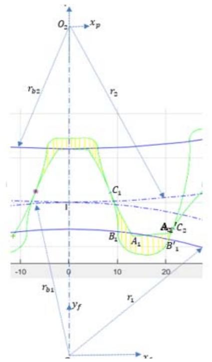 Figure 5: Leakage surface at a location where profiles are in contact When the profiles are not in contact, the radial leakage surfaces are non-zero and, consequently the axial leakage surface has as its boundary the tooth profiles and the minimum distances between the adjacent profiles. The figure 6 below is an illustration of this situation. 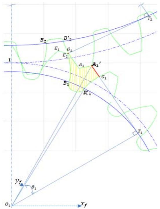 Figure 6: Radial and axial leakage Surfaces at a location where profiles are not in contact ### f) Information Technology Tools The simulation of the equations and the model obtained was carried out with the MATLAB R2016A application installed in an HP computer, AMD A6-3400 APU HD Graphics 1.40 GHz; 6 GB of RAM. ## III. METHOD ### a) Hypothesis Our study was carried out under the following assumptions: - The portion of tooth between the addendum circle and the base circle is in involute. - The shape of the tooth portion after the base circle varies depending on the tooth number. - Radial distances are minimum distances between adjacent profiles. - The direction of rotation of positive angles is the trigonometric direction and, the direction of rotation of negative angles is the anti-trigonometric direction. - In our calculations, the initial position $(\phi_{i} = 0)$ is the position where the two adjacent profiles meet at the common point of the pitch circles. However, for the presentation and the comparative study of the results, we bring the initial position back to the position where $(O_{1}O_{2})$ passes simultaneously through the midpoints of the gear top land and the pinion root. ### b) Calculation Algorithm From the geometric parameters of a gear tooth, the parametric equations of the half tooth profile are established. The complete gear tooth is obtained by axial symmetry of this half tooth, followed by N-1 successive rotations of the primary tooth with respect to the axis of the gear and respective angles $2^{\star}\pi^{\star}\mathrm{k} / \mathrm{N}$, $1\leq k\leq N - 1$. Where N is the number of teeth. From the initial position, the coordinates of the boundary points of the leakage surfaces are calculated as a function of the rotation angle. From the properties of the involute of a circle, we calculate the radial distances as a function of the rotation angle and by surface integration, we obtain the radial surfaces. The figure 7 below is the algorithm that succinctly presents our working methodology. 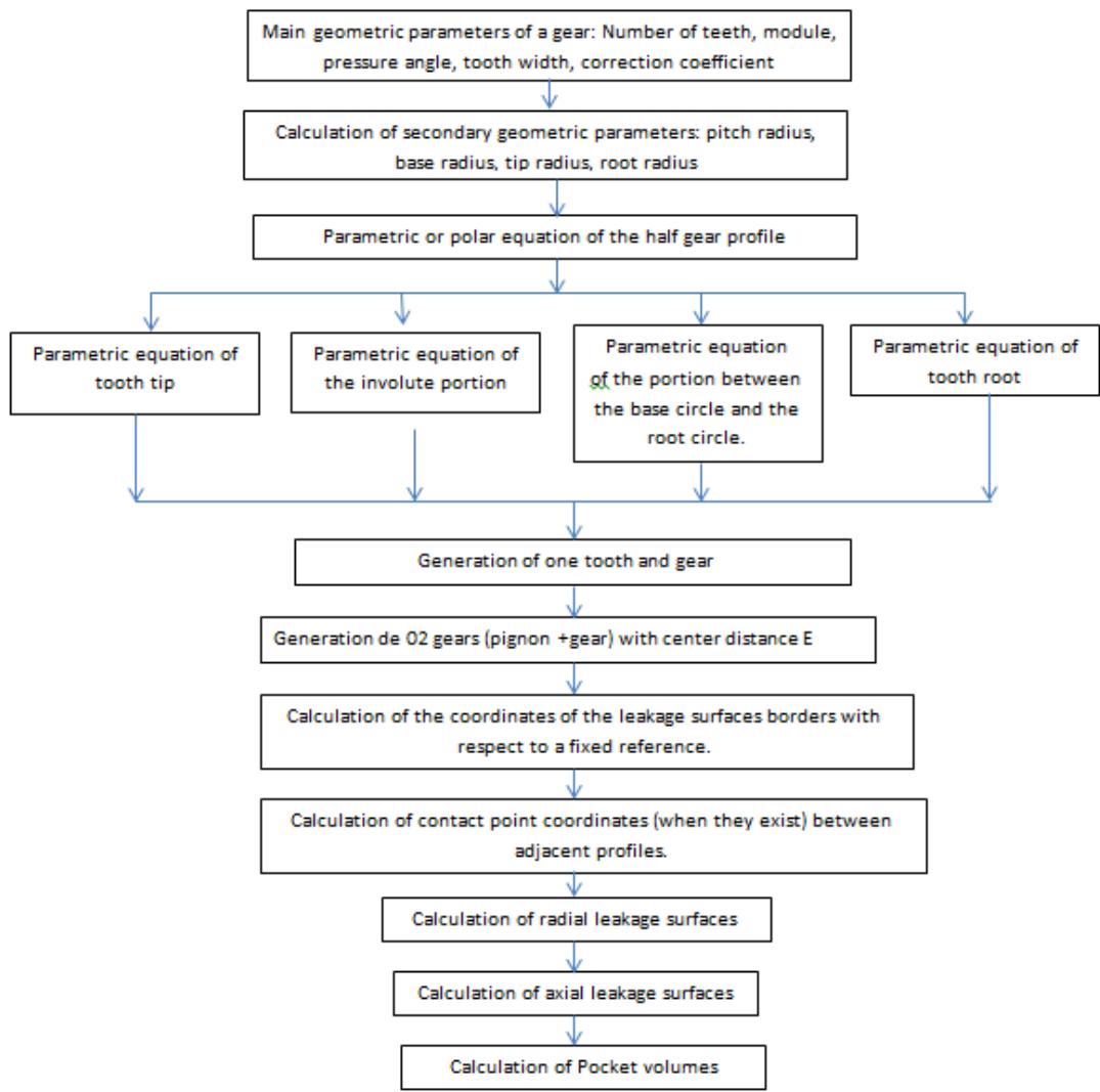 Figure 7: A calculation algorithm ### c) Half Tooth Modeling This modeling is carried out based on the tooth profile shown in Figure 4. #### 1) Tooth tip equation The tooth tip is a fraction of the tip circle (see figure 4). By applying the parametric equation of a circle with radius $r_a$ (tip radius) centered in the point $O_1$, the parametric equation of the half of the geartooth tip is given in the coordinate system $(0, x, y)$ by the relation (1) below: $$ \left\{ \begin{array}{l} x(q) = r_{a} * \sin(q) \\ y(q) = r_{a} * \cos(q) \end{array} \right. \tag{1} $$ With $q_{min} \leq q \leq q_{max}$, $q_{min} = \operatorname{mes}\left(\vec{i}, \overrightarrow{OA}\right)$ and $q_{max} = \frac{\pi}{2}$ #### 2) Equations of the involute portion (AB) By applying the properties of the involute of the circle, the parametric equations of the portion (AB) in the fixed frame $(\mathsf{O},\mathsf{x},\mathsf{y})$ are given by the relation (2) below: $$ \left\{ \begin{array}{l} x (\theta) = - r _ {b} (\sin (\theta) - \theta \cos (\theta)) \\ (a) \end{array} \right\} \tag{2} $$ $$ \left\lfloor y (\theta) = r _ {b} \left(\cos (\theta) + r _ {b} \theta \sin (\theta)\right) $$ with $0 \leq \theta \leq [r_a^2 - 1]^{1/2}$. 3. Equations of the portion between the base circle and the root circle. On the figure 6, $$ 0 \leq \zeta \leq \zeta_ {\max } \tag {3} $$ with $\zeta_{max} = \frac{\pi}{N} -\Omega_s$ By application of the geometric construction properties (see[20]) $\zeta = \arccos (2\mathrm{rb}^{\star}\mathrm{rp} / (rb^{2} + rp^{2}))$ In the case of gears with pressure angle $\alpha = 20^{\circ}$, when $\zeta_{max} \leq \arccos(2rb^*rp / (rb^2 + rp^2))$ then we take $\zeta = k^*((\pi/N) - \Omega_s)$; $0 < k \leq 1$. In summary, in the portion between the base circle and the root circle 03 possible profiles shapes emerge depending on the number of teeth: - If $r_b \leq r_p$: The circular portion does not exist. Our tooth will consist only of the involute part and the tooth top. - If $r_b > r_p$: Two possibilities emerge. - If $\arccos (2r_b^* r_p / (r_b^2 + r_p^2)) \leq \zeta_{max}$: In this case, this portion will consist of two (02) types of profiles, namely the arc of a circle BD followed by the root circle. - If $\zeta_{\text{max}} < \arccos(2r_b^\star r_p / (r_b^2 + r_p^2))$: In this case, this portion is broken down into segment [BC] and arc of circle CD followed by the part of the root circle. ## i. Case where $\arccos (2\mathbf{r}_{\mathrm{b}}^{\star}\mathbf{r}_{\mathrm{p}} / (\mathbf{r}_{\mathrm{b}}^{2} + \mathbf{r}_{\mathrm{p}}^{2}))\leq \zeta_{\max}$ Equation of segment [BC] in (o, x, y) As a reminder, segment [BC] only exists when $N < 25$ teeth. This segment equation requires knowledge of the coordinates of points B and C. According to figure 5, the coordinates of point B are given by the relation (4) below: $$ \left\{ \begin{array}{l} \mathrm{x B} = \operatorname{rbsin} \left(\Omega_{s}\right) \\ \mathrm{y B} = \operatorname{rbcos} \left(\Omega_{s}\right) \end{array} \right. \tag{4} $$ With $\Omega_{s} = \mathrm{inv}(\alpha_{0}) + \beta_{1}$ and $\xi = k^{\star}((\pi /N) - \Omega_s)$. $0 < k\leq 1$ $\beta_{i}$ is the angle between axis $(O_{1}O_{2})$ and $(O_{i},y_{i})$ with axis $(O_{i},y_{i})$ dividing the tooth of gear i in two equal parts. $\beta_{i} = \frac{t_{si}}{2r_{i}}$ with $t_{si} = \frac{\pi m}{2} + 2^* e^*\tan(\alpha)$. $t_{si}$: tooth thickness at the standard pitch circle, $\alpha$: pressure angle, m: module, e: profile shift, $-0.5 \leq \mathrm{e} / \mathrm{m} \leq 1$. The coordinates of point D are given by relation (5) below: $$ \left\{ \begin{array}{l} \mathrm{x D} = \mathrm{r p} * \sin \left(\Omega_{s} + \zeta\right) \\ \mathrm{y D} = \mathrm{r p} * \cos \left(\Omega_{s} + \zeta\right) \end{array} \right. \tag{5} $$ Let $K$ be the contact point between the tangent to $\widetilde{CD}$ in $D$ and the tangent to the involute in $B$. Then the coordinates of $K$ are given by relation (6) below: $$ \left\{ \begin{array}{c} \mathrm{x K} = (\mathrm{r p} * \tan(\Omega_{s})) / (\cos(\Omega_{s} + \zeta) + (\sin(\Omega_{s} + \zeta)) * \tan(\Omega_{s})) \\ \mathrm{y k} = \mathrm{x k} / \tan(\Omega_{s}) \end{array} \right. \tag{6} $$ Let's posed $1 = \text{sqrt}((\text{(xD - xk)} \wedge 2) + (\text{(yD - yk)} \wedge 2))$ and $d2 = \text{sqrt}((xk)^2 + (yk)^2)$. The coordinates of point C are given by relation (7) below: $$ \left\{ \begin{array}{l} x C = (d 1 + d 2) * \sin \left(\Omega_{s}\right) \\ y C = (d 1 + d 2) * \cos \left(\Omega_{s}\right) \end{array} \right. \tag{7} $$ The following relation (8) is the parametric equation of the segment [BC] in $(0, x, y)$: $$ \left\{ \begin{array}{l} x = d \\ y = a * d \end{array} \right. \tag{8} $$ With $xC \leq d \leq xB$ et $a = yB / xB = yC / xC$; The following relation (9) gives us the coordinates of the center of curvature $E$ of the arc $\widetilde{CD}$: $$ \left\{ \begin{array}{l} \mathrm{x E} = (\mathrm{r p} + \mathrm{r c} 1) * \sin \left(\Omega_{s} + \zeta\right) \\ \mathrm{y E} = (\mathrm{r p} + \mathrm{r c} 1) * \cos \left(\Omega_{s} + \zeta\right) \end{array} \right. \tag{9} $$ With rc1 = d1 * tan((pi/4) + (\\zeta/2)). rc1 is the radius of curvature of the arc $\widetilde{CD}$. Equation of arc $\widetilde{CD}$ in the reference $(o, x, y)$ The Equation of the arc $\widetilde{CD}$ in the reference $(0, x, y)$ is given by the relation (10) below: $$ \left\{ \begin{array}{l} \mathrm{x} (\mathrm{q}) = \mathrm{x E} + \mathrm{r c 1} * \sin (\mathrm{q}) \\ \mathrm{y} (\mathrm{q}) = \mathrm{y E} + \mathrm{r c 1} * \cos (\mathrm{q}) \end{array} \right. \tag{10} $$ With $q_{\min} \leq q \leq q_{\max}$, $q_{\min} = \operatorname{mes}(\vec{i}, \overrightarrow{EC})$ and $q_{\max} = \operatorname{mes}(\vec{i}, \overrightarrow{ED})$ Equation of the circular portion between $D$ and the tip circle in $(o, x, y)$ This portion is a fraction of the root circle. Its equation is given by relation (11) below: $$ \left\{ \begin{array}{l} \mathrm{x}(\mathrm{q}) = \mathrm{r p} * \sin(\mathrm{q}) \\ \mathrm{y}(\mathrm{q}) = \mathrm{r p} * \cos(\mathrm{q}) \end{array} \right. \tag{11} $$ with qmin $\leq$ q $\leq$ qmax; qmin $= \frac{\pi}{2} -\frac{\pi}{N}$ and qmax= mes $(\vec{t},\overrightarrow{OD})$ ii. Case where $\arccos (2\mathrm{rb}^{\star}\mathrm{rp} / (rb^{2} + rp^{2}))\leq \zeta_{max}$: the segment [BC] does not exist In this case, the center of curvature is given by the relation (12) below: $$ \left\{\begin{array}{c}\mathrm {x E} = \mathrm {r b} * \tan \left(\Omega_{s} + \zeta\right) / \left(\cos \left(\left(\Omega_{s}\right) + \sin \left(\Omega_{s}\right) * \tan \left(\Omega_{s} + \zeta\right)\right) \right.\\\mathrm {y E} = r b / \left( \cos \left(\left(\Omega_{s}\right) + \sin \left(\Omega_{s}\right) * \tan \left(\Omega_{s} + \zeta\right)\right)\right.\end{array}\right. \tag {12} $$ Where $\zeta = \arccos (2\mathrm{rb}^{\star}\mathrm{rp} / (rb^{2} + rp^{2}))$ The equation of the arc $\widetilde{CD}$ in the reference $(0, x, y)$ is given by the relation (10) below, with the curvature radius $rc1 = ED = EB$. ### d) Gear Generating For the generation of a complete gear wheel, the following methodology has been adopted: - Codification on Matlab of the equations developed above (half of a tooth). - Application of symmetry with respect to $(0, \vec{J})$ to get a whole tooth. - Generating of N-1 others teeth by N-1 successive rotations of the initial tooth of respective angles $(2^{\star}\pi /N)^{\star}i$, with $1\leq i\leq N - 1$ e) Calculation of Radial and Axial Leakage Surfaces i. Calculation of the border points coordinates at a given position (see figures 5 and 6). At a rotation angle $\phi_{i}$ around $O_{i}$ with respect to the initial position, the coordinates of points A1, A1', E1, E1', B1, and B1' (see figures 5 and 6) in $(O_{f}, x_{f}, y_{f})$ are given by equations below: The coordinates of the tooth tip corner of gear in $(O_f, x_f, y_f)$ are given by relations (14) and (15) below: $$ \left\{ \begin{array}{l} x A _ {1} = \operatorname{ra 2} * \sin \left(\operatorname{inv} \left(\phi_ {r a 2}\right) - \operatorname{inv} \left(\alpha_ {0}\right) + \phi_ {2}\right) \\ y A _ {1} = E - \operatorname{ra 2} * \cos \left(\operatorname{inv} \left(\phi_ {r a 2}\right) - \operatorname{inv} \left(\alpha_ {0}\right) + \phi_ {2}\right) \end{array} \right. \tag{13} $$ with $\phi_{rai} = \operatorname{arccos}(\operatorname{rbi}/\operatorname{rai})$, $i = 1,2$ and $\operatorname{inv}(\alpha_0) = \tan (\alpha_0) - \alpha_0$ $$ \left\{ \begin{array}{l} x A _ {1} ^ {\prime} = \operatorname{ra2} * \sin \left(- \operatorname{inv} \left(\phi_{ra2}\right) + \operatorname{inv} \left(\alpha_{0}\right) + 2 * \beta_{2} + \phi_{2}\right) \\ y A _ {1} ^ {\prime} = E - ra2 * \cos \left(- \operatorname{inv} \left(\phi_{ra2}\right) + \operatorname{inv} \left(\alpha_{0}\right) + 2 * \beta_{2} + \phi_{2}\right) \end{array} \right. \tag{14} $$ With $\phi_{rai} = \arccos (\mathrm{rbi / rai})$ $i = 1,2$ Equations (16) and (17) below are the coordinates of the pinion tooth tip corner in $(O_f, x_f, y_f)$ $$ \left\{ \begin{array}{l} x E _ {1} = \operatorname{ra1} * \sin (- \operatorname{inv} (\phi_{ra1}) + \operatorname{inv} (\alpha_{0}) - 2 \theta_{ra1} - \phi_{1}) \\ y E _ {1} = \operatorname{ra1} * \cos (- \operatorname{inv} (\phi_{ra1}) + \operatorname{inv} (\alpha_{0}) - 2 \theta_{ra1} - \phi_{1}) \end{array} \right. \tag{15} $$ $$ \theta_ {r a i} = \beta_ {i} + \operatorname{inv} \left(\alpha_ {0}\right) - \operatorname{inv} \left(\phi_ {r a i}\right), i = 1, 2 $$ $$ \left\{ \begin{array}{l} x E _ {1} ^ {\prime} = \operatorname{ra1} * \sin \left(- \operatorname{inv} \left(\phi_{ra1}\right) + \operatorname{inv} \left(\alpha_{0}\right) - \phi_{1}\right) \\ y E _ {1} ^ {\prime} = \operatorname{ra1} * \sin \left(- \operatorname{inv} \left(\phi_{ra1}\right) + \operatorname{inv} \left(\alpha_{0}\right) - \phi_{1}\right) \end{array} \right. \tag{16} $$ $$ \theta_ {r a i} = \beta_ {i} + \operatorname{inv} \left(\alpha_ {0}\right) - \operatorname{inv} \left(\phi_ {r a i}\right), i = 1, 2 $$ The coordinates of $\mathsf{B}_1^{\prime}$ and $\mathsf{B}_2$ in (Of, xf, yf) are given by relations (18) and (19) below: $$ \left\{ \begin{array}{l} x B _ {1} ^ {\prime} = \operatorname {r b} 1 * \sin \left(\Omega_ {s} + \beta_ {1} + \phi_ {1}\right) \\ y B _ {1} ^ {\prime} = \operatorname {r b} 1 * \cos \left(\Omega_ {s} + \beta_ {1} + \phi_ {1}\right) \end{array} \right. \tag{17} $$ $$ \left\{ \begin{array}{l} x B _ {2} = \mathrm {r b} 2 * \sin \left(- i n v \left(\alpha_ {0}\right) + \pi - 2 \beta_ {2} - \phi_ {2}\right) \\ y B _ {2} = \mathrm {E} + \mathrm {r b} 2 * \cos \left(- i n v \left(\alpha_ {0}\right) + \pi - 2 \beta_ {2} - \phi_ {2}\right) \end{array} \right. \tag {18} $$ When $r_b \leq r_p$, the Coordinates of the contact points between the tooth profile and the root circle are given by the equation (19) below: $$ \left\{ \begin{array}{l} x p _ {1} = \operatorname {r p} 1 * \sin \left(\Omega_ {s} - \tan (\mathrm {a y}) + \mathrm {a y} - \beta_ {1} - \phi_ {1}\right) \\ y p _ {1} = \operatorname {r p} 1 * \cos \left(\Omega_ {s} - \tan (\mathrm {a y}) + \mathrm {a y} - \beta_ {1} - \phi_ {1}\right) \end{array} \right. \tag {19} $$ With ay=Arccos(rb1/rp1); Coordinates of contacts points ( $C_1$ and $C_2$ of the pinion and gear (see figure 5). Existence condition of $C_1$ and $C_2$ $C_1$ exists if and only if: $$ \tan \left(\alpha_ {0}\right) - \sqrt {\left(\frac {r _ {a 1}}{r _ {b 1}}\right) ^ {2} - 1} \leq \phi_ {1} \leq - \frac {r _ {s 2}}{r _ {s 1}} (\tan \left(\alpha_ {0}\right) - \sqrt {\left(\frac {r _ {a 2}}{r _ {b 2}}\right) ^ {2} - 1}) \tag {20} $$ In this case, the radial surface 1 is zero: $S_{\mathrm{r1}} = 0$ $C_2$ exists if and only if: $$ \left(- \frac {r _ {s 2}}{r _ {s 1}}\right) \left(- \tan \left(\alpha_ {0}\right) - 2 \beta_ {2} + \sqrt {\left(\frac {r _ {a 2}}{r _ {b 2}}\right) ^ {2} - 1}\right) \leq \phi_ {1} \leq - \tan \left(\alpha_ {0}\right) + 2 \beta_ {1} + \sqrt {\left(\frac {r _ {a 1}}{r _ {b 1}}\right) ^ {2} - 1} \tag {21} $$ In this case, the radial distance 2 is zero: $S_{r2} = 0$. At the initial condition, $\mathsf{C}_1$ is confused with I. By applying the line of contact between the two conjugate surfaces, we obtain the coordinates of points $C_i$ rotation angle $\phi_{\mathrm{i}}$ around $0_{\mathrm{i}}$ with respect to the initial position in $(O_f, x_f, y_f)$: Then the coordinates of $C_1$ in $(O_f, x_f, y_f)$ are given by the relation (22) below: $$ \left\{ \begin{array}{l} x C _ {1} = \operatorname{r b} 1 * \left(\sqrt{1 + \theta_ {C 1} {} ^ {2}}\right) \sin \left(\operatorname{Arctan} \left(\theta_ {C 1}\right) - \theta_ {C 1} + \operatorname{inv} \left(\alpha_ {0}\right) - \phi_ {1}\right) \\ y C _ {1} = \operatorname{r b} 1 * \left(\sqrt{1 + \theta_ {C 1} {} ^ {2}}\right) \cos \left(\operatorname{Arctan} \left(\theta_ {C 1}\right) - \theta_ {C 1} + \operatorname{inv} \left(\alpha_ {0}\right) - \phi_ {1}\right) \end{array} \right. \tag{22} $$ with $\theta_{C1} = \tan (\alpha_0) - \phi_1$ The coordinates of $C_2$ in $(O_f, x_f, y_f)$ are given by the relation (23) below: $$ \left\{ \begin{array}{l} x C _ {2} = \operatorname{r b} 1 * \left(\sqrt{1 + \theta_ {C 2} {} ^ {2}}\right) \sin \left(- \operatorname{Arctan} \left(\theta_ {C 2}\right) + \theta_ {C 2} - \operatorname{inv} \left(\alpha_ {0}\right) + 2 \beta_ {1} - \phi_ {1}\right) \\ y C _ {2} = \operatorname{r b} 1 * \left(\sqrt{1 + \theta_ {C 2} {} ^ {2}}\right) \cos \left(- \operatorname{Arctan} \left(\theta_ {C 2}\right) + \theta_ {C 2} - \operatorname{inv} \left(\alpha_ {0}\right) + 2 \beta_ {1} - \phi_ {1}\right) \end{array} \right\} \tag{23} $$ with $\theta_{C2} = \tan (\alpha_0) - 2\beta_1 + \phi_1$ In $(O_p, x_p, y_p)$, the coordinates of $C_1$ are given by the relation (24) below: $$ \left\{ \begin{array}{l} x C _ {1} = \operatorname{r b} 2 * \left(\sqrt{1 + \theta^ {\prime} {} _ {C 1} {} ^ {2}}\right) \sin \left(\operatorname{Arctan} \left(\theta^ {\prime} {} _ {C 1}\right) - \theta^ {\prime} {} _ {C 1} + \operatorname{inv} \left(\alpha_ {0}\right) - \pi - \phi_ {2}\right) \\ y C _ {1} = \operatorname{r b} 2 * \left(\sqrt{1 + \theta^ {\prime} {} _ {C 1} {} ^ {2}}\right) \cos \left(\operatorname{Arctan} \left(\theta^ {\prime} {} _ {C 1}\right) - \theta^ {\prime} {} _ {C 1} + \operatorname{inv} \left(\alpha_ {0}\right) - \pi - \phi_ {2}\right) \end{array} \right\} \tag{24} $$ with $\theta^{\prime}_{C1} = \tan (\alpha_{0}) - \phi_{2}$ In (Op, xp, yp), the coordinates of $C_2$ are given by the relation (25) below: $$ \left\{ \begin{array}{l} x C _ {2} = \operatorname{r b} 2 * \left(\sqrt{1 + \theta^ {\prime} {} _ {C 2}}\right) ^ {2} \sin \left(- \operatorname{Arctan} \left(\theta^ {\prime} {} _ {C 2}\right) + \theta^ {\prime} {} _ {C 2} - \operatorname{inv} \left(\alpha_ {0}\right) + \pi - 2 \beta_ {2} - \phi_ {2}\right) \\ y C _ {2} = \operatorname{r b} 2 * \left(\sqrt{1 + \theta^ {\prime} {} _ {C 2}}\right) ^ {2} \cos \left(- \operatorname{Arctan} \left(\theta^ {\prime} {} _ {C 2}\right) + \theta^ {\prime} {} _ {C 2} - \operatorname{inv} \left(\alpha_ {0}\right) + \pi - 2 \beta_ {2} - \phi_ {2}\right) \end{array} \right. \tag{25} $$ with $\theta^{\prime}_{C2} = \tan (\alpha_0) + 2\beta_2 + \phi_2$ $$ O_1C_2 = \mathrm{rb}1 * \left(\sqrt{1 + \theta_{C2}^2}\right); O_2C_2 = \mathrm{rb}2 * \left(\sqrt{1 + \theta_{C2}^{'2}}\right), O_1C_1 = \mathrm{rb}1 * \left(\sqrt{1 + \theta_{C1}^2}\right); \quad O_2C_1 = \mathrm{rb}2 * \left(\sqrt{1 + \theta_{C1}^{'2}}\right) $$ ## ii. Calculation of Radial Leakage Surfaces The radial leakage surfaces vary in function of the rotation angle of gear. For the calculation of the radial leakage surfaces we will distinguish 05 possibilities: - When $C_1$ and $C_2$ exist, i.e., when the profiles touch each other simultaneously. In this case the surfaces $S_{r1}$ and $S_{r2}$ are simultaneously zero. - When we are at the left of the initial position, and only $C_2$ exists ( $S_{r1} > 0$ and $S_{r2} = 0$ ), - When we are at the left of the initial position with $C_1$ and $C_2$ does not exist $(S_{r1} > 0$ and $S_{r2} > 0)$ - When we are at the right of the initial position and only $C_2$ exists ( $S_{r1} = 0$ and $S_{r2} > 0$ ), - When we are at the right of the initial position with $C_1$ and $C_2$ does not exist $(S_{r1} > 0$ and $S_{r2} > 0)$ The relations below give the expressions of the radial leakage surfaces in each of these cases cited above. At the right of the initial position Case where $S_{r1} = 0$ and $S_{r2} > 0$: $$ (\tan(\alpha_{0}) - \sqrt{(\frac{r_{a1}}{r_{b1}})^{2} - 1} < \phi_{1} < (-\frac{r_{s2}}{r_{s1}})(-\tan(\alpha_{0}) - 2\beta_{2} + \sqrt{(\frac{r_{a2}}{r_{b2}})^{2} - 1})) $$ According to figure 5, $$ \mathrm {S} _ {\mathrm {r} 2} = b * A _ {2} G _ {1} \tag {26} $$ where $b$ is the face of the tooth width. $$ A_{2}G_{1}=A_{2}T_{1}-G_{1}T_{1} $$ with $A_{2}T_{1} = \sqrt{O_{1}A_{2}^{2} - rb_{1}^{2}}$, $G_{1}T_{1} = rb_{1}\theta_{1}$ $$ \theta_ {1} = \operatorname{mes} (\overrightarrow{O _ {1} A _ {2}}, \overrightarrow{O _ {1} T _ {1}}) - \operatorname{mes} (\overrightarrow{O _ {1} A _ {2}}, \overrightarrow{O _ {1} B _ {1} ^ {\prime}}) \text{and} \operatorname{mes} (\overrightarrow{O _ {1} A _ {2}}, \overrightarrow{O _ {1} T _ {1}}) = \operatorname{arccos} (\frac{r b _ {1}}{O _ {1} A _ {2}}) $$ $$ \operatorname{mes} \left(\overrightarrow{O _ {1} A _ {2}}, \overrightarrow{O _ {1} B _ {1} ^ {\prime}}\right) = \operatorname{mes} (\vec{i}, \overrightarrow{O _ {1} A _ {2}}) - \operatorname{mes} (\vec{i}, \overrightarrow{O _ {1} B _ {1} ^ {\prime}}) \tag{28} $$ with $\mathrm{mes}(\vec{t},\overrightarrow{O_1A_2}) = \mathrm{arccos}((\mathrm{(x}A_2 - 0)(1 - 0)) / O_1A_2)$ and $\mathrm{mes}(\vec{t},\overrightarrow{O_1B'_1}) = \mathrm{arccos}((\mathrm{(x}B'_1 - 0)(1 - 0)) / O_1B'_1)$. Case where $S_{r1} > 0$ and $S_{r2} > 0$: $(\phi_1 < \tan(\alpha_0) - \sqrt{(\frac{r_1}{r_1})^2 - 1})$ According to figure 6, $$ \mathrm {S} _ {\mathrm {r} 1} = b * E _ {2} G _ {2} \tag {29} $$ $$ E_{2}G_{2} = E_{2}T_{2} - G_{2}T_{2} $$ $$ E _ {2} T _ {2} = \sqrt{O _ {2} E _ {2} ^ {2} - r b _ {2} ^ {2}}, G _ {2} T _ {2} = r b _ {2} \theta_ {2}, \theta_ {2} = \operatorname{mes} (\overrightarrow{O _ {2} E _ {2}}, \overrightarrow{O _ {2} T _ {2}}) - \operatorname{mes} (\overrightarrow{O _ {2} E _ {2}}, \overrightarrow{O _ {2} J _ {2}}) $$ with $\mathrm{mes}(\overrightarrow{O_2E_2},\overrightarrow{O_2T_2}) = \mathrm{Arccos}\left(\frac{rb_2}{O_2E_2}\right)$ $$ \operatorname{mes} \left(\overrightarrow{O _ {2} E _ {2}}, \overrightarrow{O _ {2} J _ {2}}\right) = \operatorname{mes} (\vec{i}, \overrightarrow{O _ {2} E _ {2}}) - \operatorname{mes} (\vec{i}, \overrightarrow{O _ {2} J _ {2}}) \tag{31} $$ $\mathrm{mes}(\vec{i}, \overrightarrow{O_2E_2}) = \arccos (((xE_2 - 0)(1 - 0)) / O_2E_2)$ and $\mathrm{mes}(\vec{i}, \overrightarrow{O_2J_2}) = \arccos (((xJ_2 - 0)(1 - 0)) / O_2J_2)$ Sr1 is given by the relation (27) At the left of the initial position Case where $S_{r1} > 0$ and $S_{r2} = 0$: $$ \left(\left(- \tan \left(\alpha_ {0}\right) + 2 \beta_ {1} + \sqrt {\left(\frac {r _ {a 1}}{r _ {b 1}}\right) ^ {2} - 1}\right) > \phi_ {1} > \frac {r _ {s 2}}{r _ {s 1}} \left(\tan \left(\alpha_ {0}\right) - \sqrt {\left(\frac {r _ {a 2}}{r _ {b 2}}\right) ^ {2} - 1}\right)\right) $$ Like the previous cases, $$ S_{r1} = b * A_{2}^\prime G_{1}^\prime $$ $$ A_{2}^\prime G_{1}^\prime = A_{2}^\prime T_{1}^\prime - G_{1}^\prime T_{1}^\prime \tag{33} $$ with $A_{2}^{\prime}T_{1}^{\prime} = \sqrt{O_{1}A_{2}^{\prime 2} - rb_{1}^{2}}$, $G_{1}^{\prime}T_{1}^{\prime} = rb_{1}\theta_{1}^{\prime}$, $\theta_{1}^{\prime} = \mathrm{mes}(\overrightarrow{O_{1}A_{2}^{\prime}},\overrightarrow{O_{1}T_{1}^{\prime}})$ - $\mathrm{mes}(\overrightarrow{O_{1}A_{2}^{\prime}},\overrightarrow{O_{1}J_{1}^{\prime}})$ and $\mathrm{mes}(\overrightarrow{O_{1}A_{2}^{\prime}},\overrightarrow{O_{1}T_{1}^{\prime}})$ $= \operatorname{arccos}\left(\frac{rb_{1}}{O_{1}A_{2}^{\prime}}\right)$ $$ \operatorname{mes} \left(\overrightarrow{O _ {1} A ^ {\prime}} _ {2}, \overrightarrow{O _ {1} J ^ {\prime}} _ {1}\right) = \operatorname{mes} (\vec{i}, \overrightarrow{O _ {1} A ^ {\prime}} _ {2}) - \operatorname{mes} (\vec{i}, \overrightarrow{O _ {1} J ^ {\prime}} _ {1}) \tag{34} $$ $\mathrm{mes}(\vec{t}, \overrightarrow{O_1A'_2}) = \mathrm{arccos}((\mathrm{x}A'_2 - 0)(1 - 0)) / O_1A'_2)$ and $\mathrm{mes}(\vec{t}, \overrightarrow{O_1J'_1}) = \mathrm{arccos}((\mathrm{x}J'_1 - 0)(1 - 0)) / O_1J'_1)$ Case where $S_{r1} > 0$ and $S_{r2} > 0$ ( $\phi_1 > -\tan(\alpha_0) + 2\beta_1 + \sqrt{\frac{r_a1}{r_b1}}^2 - 1$ ) $$ \mathrm {S} _ {\mathrm {r} 2} = b * E _ {2} ^ {\prime} G _ {2} ^ {\prime} \tag {35} $$ with $E^{\prime}_{2}G^{\prime}_{2} = E^{\prime}_{2}T^{\prime}_{2}\cdot G^{\prime}_{2}T^{\prime}_{2},E^{\prime}_{2}T^{\prime}_{2} = \sqrt{O_{2}E^{\prime}_{2}{}^{2} - rb_{2}{}^{2}}$ $G^{\prime}_{2}T^{\prime}_{2} = rb_{2}\theta_{2}$ and $$ \theta^ {\prime} _ {2} = \operatorname{mes} (\overrightarrow{O _ {2} E ^ {\prime}} _ {2}, \overrightarrow{O _ {2} T ^ {\prime}} _ {2}) - \operatorname{mes} (\overrightarrow{O _ {2} E ^ {\prime}} _ {2}, \overrightarrow{O _ {2} J ^ {\prime}} _ {2}), \operatorname{mes} (\overrightarrow{O _ {2} E ^ {\prime}} _ {2}, \overrightarrow{O _ {2} T ^ {\prime}} _ {2}) = \operatorname{arccos} (\frac{r b _ {2}}{O _ {2} E ^ {\prime}}) $$ $$ \operatorname{mes} \left(\overrightarrow{O _ {2} E ^ {\prime}} _ {2}, \overrightarrow{O _ {2} J ^ {\prime}} _ {2}\right) = \operatorname{mes} (\vec{t}, \overrightarrow{O _ {2} E ^ {\prime}} _ {2}) - \operatorname{mes} (\vec{t}, \overrightarrow{O _ {2} J ^ {\prime}} _ {2}) \tag{36} $$ $\mathrm{mes}(\vec{t},\overrightarrow{O_2E'_2}) = \mathrm{arccos}((\mathrm{x}E'_2 - 0)(1 - 0)) / O_2E'_2)$ and $\mathrm{mes}(\vec{t},\overrightarrow{O_2J'_2}) = \mathrm{Arccos}((\mathrm{x}J'_2 - 0)(1 - 0)) / O_2J'_2)$ Sr1 is given by relation (33) ## iii. Calculation of Axial Leakage Surfaces Case where $S_{r1} = 0$ and $S_{r2} = 0$: $$ \left(\left(- \frac {r _ {s 2}}{r _ {s 1}}\right) (- \tan (\alpha_ {0}) - 2 \beta_ {2} + \sqrt {\binom {r _ {a 2}} {r _ {b 2}} ^ {2} - 1}\right) \leq \phi_ {1} \leq - \frac {r _ {s 2}}{r _ {s 1}} (\tan (\alpha_ {0}) - \sqrt {\binom {r _ {a 2}} {r _ {b 2}} ^ {2} - 1})) $$ Case where $r_p < r_b$ According to figure 5 and figure 6: $$ \text{Surface} = \mathrm{S C} _ {1} B _ {1} B ^ {\prime} _ {1} C _ {2} A _ {1} A ^ {\prime} _ {1} C _ {1} = \mathrm{S O} _ {1} C _ {1} A _ {1} A ^ {\prime} _ {1} C _ {2} O _ {1} - \mathrm{S O} _ {1} C _ {1} B _ {1} B ^ {\prime} _ {1} C _ {2} O _ {1} \tag{37} $$ $$ \mathrm{S O} _ {1} \mathrm{C} _ {1} \mathrm{A} _ {1} \mathrm{A} ^ {\prime} _ {1} \mathrm{C} _ {2} \mathrm{O} _ {1} = \text{triangle} \_ \mathrm{O} _ {1} \mathrm{C} _ {2} \mathrm{O} _ {2} \mathrm{O} _ {1} - \text{triangle} \_ \mathrm{O} _ {1} \mathrm{C} _ {1} \mathrm{O} _ {2} \mathrm{O} _ {1} - \mathrm{S O} _ {2} \mathrm{C} _ {2} \mathrm{A} _ {1} \mathrm{A} ^ {\prime} _ {1} \mathrm{C} _ {1} \mathrm{O} _ {2} \tag{38} $$ Avec triangle $O_{1}C_{2}O_{2}O_{1} = 0.5O_{1}C_{2}^{*}E^{*}\sin (\theta_{C2})$ et triangle $\begin{array}{r}O_{1}C_{1}O_{2}O_{1} = 0.5^{*}O_{1}C_{1}^{*}E^{*}\sin (\theta_{C1}) \end{array}$ $$ SO_{2}C_{2}A_{1}A_{1}^{ extprime}C_{1}O_{2} = SO_{2}C_{2}A_{1}^{ extprime}O_{2} + SO_{2}C_{2}A_{1}^{ extprime}A_{1}O_{2} + SO_{2}A_{1}C_{1}O_{2} $$ $$ \mathsf{S O} _ {2} C _ {2} A _ {1} ^ {\prime} A _ {1} O _ {2} = 0.5 * r _ {a 2} ^ {2} * (2 * \theta_ {r a 2}), \mathsf{S O} _ {2} A _ {1} C _ {1} O _ {2} = 0.5 * r _ {b 2} ^ {2} ((\sqrt{\binom{r _ {a 2}} {r _ {b 2}}} ^ {2} - 1) ^ {3} - \theta_ {C 2} ^ {3}) / 3 $$ and $\mathsf{SO}_2C_2A'_1O_2 = 0.5^* r_{b2}^2\cdot (\sqrt{\left(\frac{r_{a2}}{r_{b2}}\right)^2 - 1})^3 -\theta'_C2^3) / 3$ $$ S O _ {1} C _ {1} B _ {1} B ^ {\prime} _ {1} C _ {2} O _ {1} = S O _ {1} C _ {1} B _ {1} O _ {1} + S O _ {1} B _ {1} B ^ {\prime} _ {1} O _ {1} + S O _ {1} B ^ {\prime} _ {1} C _ {2} O _ {1} \tag {40} $$ with $SO_1C_1B_1O_1 = 0.5^{\star}\mathbf{rb}1^{2\star}(\theta_{C1}{}^3) / 3,$ $$ SO_1B_1B'_1O_1 = (rc1 + rp1) * o1c * sin(\zeta) - rc1^2 * (qmax - qmin) + rp1^2 * (q2max - q2min) $$ $$ O _ {1} \mathrm {c} = \sqrt {\left(x _ {c} - 0\right) ^ {2} + \left(y _ {c}\right) ^ {2}} $$ $$ q 2 \max = (\pi / 2) - (\zeta + \Omega_ {s}) and q 2 \min = (\pi / 2) - (\pi / N 1) $$ $$ \begin{array}{l} \operatorname{qmin} = \operatorname{Arccos} \left(\left(1 * \left(x _ {B} - x _ {E}\right) + 0 * \left(y _ {B} - y _ {E}\right)\right) / \mathrm{E B}\right) \text{and} \operatorname{qmax} = \operatorname{qmin} + \operatorname{acos} \left(\left(\left(x _ {C} - x _ {E}\right) * \left(x _ {D} - x _ {E}\right) + \left(y _ {C} - y _ {E}\right) * \left(y _ {D} - y _ {E}\right)\right) / \mathrm{r c} 1 ^ {2}\right) \\\mathrm{S O} _ {1} \mathrm{B} ^ {\prime} _ {1} \mathrm{C} _ {2} \mathrm{O} _ {1} = 0.5 * \mathrm{r b} 1 ^ {2 *} \left(\theta_ {\mathrm{C} 2} {} ^ {3}\right) / 3. \\\end{array} $$ Case where $r_p \geq r_b$ According to figures 5 and 6 $$ \text{Surface} = \mathbb{S} C _ {1} p _ {1} p _ {1} ^ {\prime} C _ {2} A _ {1} A ^ {\prime} C _ {1} = \mathbb{S} O _ {1} C _ {1} A _ {1} A ^ {\prime} C _ {2} O _ {1} - \mathbb{S} O _ {1} C _ {1} p _ {1} p _ {1} ^ {\prime} C _ {2} O _ {1} \tag{41} $$ $$ \mathrm {S O} _ {1} C _ {1} p _ {1} p _ {1} ^ {\prime} C _ {2} O _ {1} = \mathrm {S O} _ {1} p _ {1} ^ {\prime} C _ {2} O _ {1} + \mathrm {S O} _ {1} p _ {1} p _ {1} ^ {\prime} O _ {1} + \mathrm {S O} _ {1} C _ {1} p _ {1} O _ {1} \tag {42} $$ with $SO_1p_1'C_2O_1 = 0.5^* \mathrm{rb}1^{2*}((\theta_{\mathrm{C2}}^3) - \theta_{\mathrm{rp1}}^3)/3, SO_1p_1p_1'O_1 = \mathrm{rp}1^{2*}(\mathrm{q3max - q2min}))$ and $q3\max = \operatorname{Arctan}(yp1 / xp1)$. $$ \mathrm{S O} _ {1} C _ {1} p _ {1} O _ {1} = 0.5 * \mathrm{r p} 1 ^ {2 \star} \left(\theta_ {C 1} ^ {3} - \theta_ {\mathrm{r p} 1} ^ {3}\right) / 3 \text{with} \theta_ {\mathrm{r p} 1} = \sqrt{\left(\frac{r _ {p 1}}{r _ {b 1}}\right) ^ {2} - 1} $$ ## IV. RESULTS ### a) Simulation Results for the Modeling of a Gear By applying the equations (1) to (13), we obtain 03 types tooth profile: - The profile made up of the gear tip, the involute part, a line segment, a circular part, and the tooth root $(r_p < r_b$ and $\arccos (2r_b^* r_p / (r_b^2 + r_p^2)) > \zeta_{max})$. - The profile made up of the gear tip, the involute part, a circular portion, and the tooth root ( $r_p < r_b$ and $\arccos(2r_b^* r_p / (r_b^2 + r_p^2)) \leq \zeta_{max}$ ). - The profile made up of the gear tip and the involute part. Here the involute part is limited at root circle $(r_b \leq r_p)$. For the application, we have chosen 03 types of gears whose respective parameters are recorded in table 1 below. Table 1: Parameters of 03 gears used for simulation <table><tr><td></td><td>Number of teeth</td><td>mmodule)</td><td>α(pressure angle)</td><td>xshift coefficeint)</td><td>b(mm)</td></tr><tr><td>Gear 1</td><td>20</td><td>10</td><td>20°</td><td>0</td><td>100</td></tr><tr><td>Gear 2</td><td>40</td><td>10</td><td>20°</td><td>-0.2</td><td>100</td></tr><tr><td>Gear 3</td><td>76</td><td>4</td><td>20°</td><td>0</td><td>100</td></tr></table> Figure 8 below is a detailed view of the half of the tooth profile taken from the simulation result for the specific case of gear 1 in table 1. 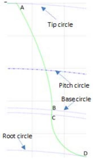 Figure 8: Detailed view of the half of tooth profile of gear 1 of table 1. Here $=93,9693\mathrm{mm}$; $=89,5\mathrm{mm}$ The particularity here is the presence of a straight part on our teeth, namely the segment [BC]. Figure 9 below is a detailed view of the half of the tooth profile taken from the simulation result for the specific case of gear 2 in table 1. 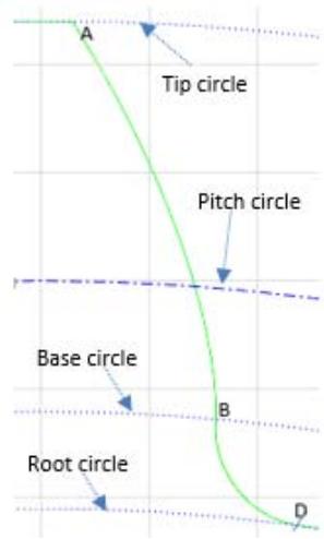 Figure 9: Detailed view of the half of the tooth of gear 2 in table 1. Here, $= 187.9385 \mathrm{~mm}$; $= 185.5 \mathrm{~mm}$ The profile is made up of the tooth top, the involute part, the circular part, and tooth root. Here, the straight part no longer exists. A detailed view of the half of the tooth profile resulting from the simulation result for the particular case of gear 3 of table 1 is represented in figure 10 below. 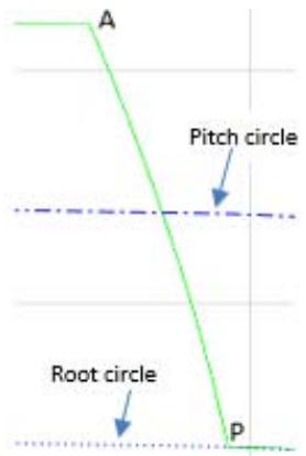 Figure 10: Detailed view of the half of the tooth in gear 3 of table 1. Here=142.8333 mm; = 147 mm In this particular case, the root radius is greater than the base radius and the tooth profile consists only of the involute part and top part. ### b) Results of Calculations of Radial and Axial Leakage Surfaces To validate our model, the simulation of our equations and formulas developed above (equations (13) to (42)) on Matlab 16 was carried out with the particular case of a gear whose characteristics are grouped in table 2 below. Table 2: Parameters of the gear used for the simulation <table><tr><td></td><td>Number of teeth</td><td>mmodule)</td><td>α(pressure angle)</td><td>xshift coefficient)</td><td>b(mm)</td></tr><tr><td>pinion</td><td>76</td><td>4</td><td>20°</td><td>0</td><td>100</td></tr><tr><td>gear</td><td>76</td><td>4</td><td>20°</td><td>0</td><td>100</td></tr></table> The application of our model for calculating of the radial leakage surfaces 1 and 2 relative to the gear of table 2 has generated the curves of figure 11 below. This figure gives the evolution of the radial leakage surfaces $(S_{r1}$ and $S_{r2})$ as a function of the rotation angle of the drive gear on the interval $[-13^{\circ}, 13^{\circ}]$. NB: To facilitate the comparative study with other models, during the simulation, we brought back the initial position at the position where $(\mathrm{O}_1\mathrm{O}_2)$ passes simultaneously through the middles of the gear tip tooth and the pinion root. That is after rotating the driver gear of $\beta_{1}$ on counterclockwise direction. 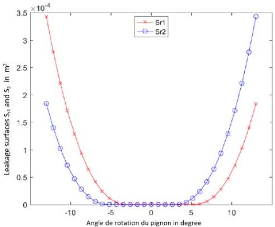 Figure 11: Evolution of the radial leakage surfaces 1 and 2 as a function of the angle of rotation of the driver gear. Case of the gearing system of table 2 The result of our model for calculating the pockets volumes corresponding to the gearing system of table 2 has generated the curve of figure 12 below. This figure gives the evolution of the pockets volumes (axial leakage surface multiplied by the tooth width) as a function of the angle of rotation of the driver gear on the interval $[-13^{\circ}, 13^{\circ}]$. 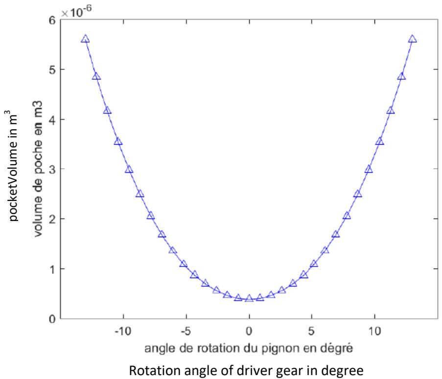 Figure 12: Radial leakage volume corresponding to the parameters in table 2 ### c) Results Interpretation The curves of Figure 11 justify the similarity of the radial and axial leakage surfaces on each side of the initial position $(\phi_{1} = 0)$. This result agrees with the surfaces evolution of figure 2. we observe that On figures 2.a) to 2.h) the axial surface reaches its minimum at the initial position $(\phi_{1} = 0)$. This observation agrees with the curve of figure 12. More we move away from the initial position $(\phi_{1} = 0)$, the pockets volumes increase. This result agrees with the observation of figures 2.a) to 2.h). The curves in figure 11 show that at the left of the initial position, the radial leakage surface one is always greater than the radial leakage surface two and, at the right of the initial position, it is the opposite phenomenon. This result agrees with the observations of figure 2. In figure 11, the two profiles bordering the radial surface $1(S_{r1})$ meet when $\phi_1$ belongs in the interval $[-3,75^\circ; 6,5^\circ]$. For the radial surface $2(S_{r1})$, this phenomenon occurs in the interval $[-6,5^\circ; 3,75^\circ]$. ## V. MODEL VALIDATION The validation of our model follows from a comparative study between the results of our model and the results of Abdelilah Lasri and al [13] and Diab Y. and al [10] for the same gear system. We have superimposed the curves of our model and those of the reference models. a) Superposition of the Radial Surfaces Curves of our Model and those Resulting from the Model of Abdelilah Lasri [13] Figure 13 below is the result of the superposition of the radial leakage surfaces (Sr1 and Sr2). In this figure, the leakage surfaces curves of our model are in blue colour and the curves of Abdelilah Lasri's model [13] are in red. 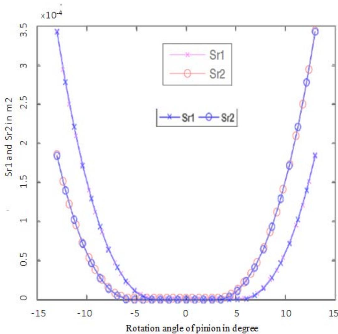 Figure 13: Superposition of radial leakage surfaces from our model (in blue) and those from Abdelilah Lasri's model \[13\](in red color) Looking at Figure 13, the radial leakage surfaces of our model and the reference model are merged. The relative deviations between the values from these two (02) models are of the order of $10^{-2}$. b) Superposition of Pocket Volume Curves from our Model and those from the Diab's Model [10] Figure 14 below is the result of the superposition of pocket volumes. On this figure, the curve of pocket volumes from our modelis blue and the Diab's model curve [10] is black. 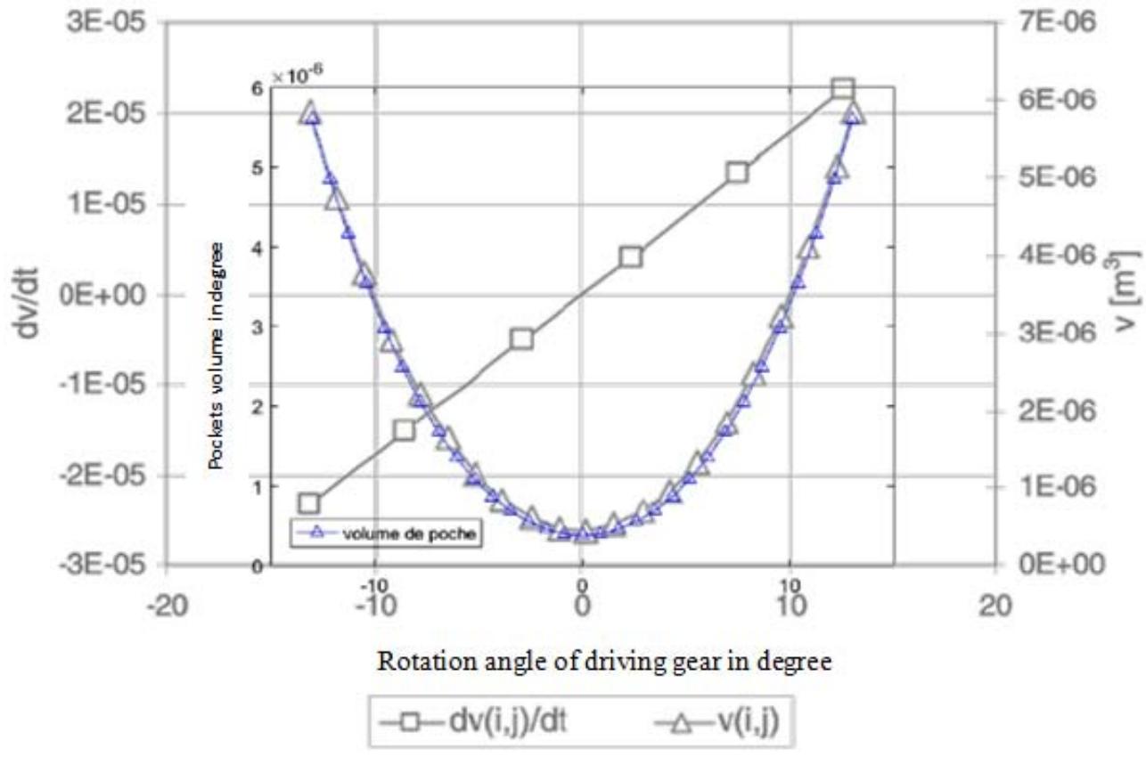 Figure 14: Superposition of pocket volumes from our model (in blue) and those from Y. Diab's[10] model (in black) On figure 14, the two curves are almost merged. In the neighbourhood of the initial position, there is a minimal difference between the 02 curves. Outside the interval $[-10^{\circ}; -10^{\circ}]$ the two curves are identical. The relative deviations between the values from the 02 curves, is at the order of $10^{-2}$. The curves of the figures 13 and 14 and the relative deviations between the results from our model and the reference models allow us to state with certainty that the model developed in this work is valid and meets our set objectives. The model developed in this work allows us to calculate the exact values of the axial and radial leakage surfaces of the lubricant in a gear. ## VI. CONCLUSION A better optimization of the power losses by the lubricant trapping in the inter-tooth space requires a preliminary work of total lifting of the veil on the gear inter-tooth space during the movement. In this perspective, we have established a purely analytical model allowing to accurately evaluating the radial and axial leakage surfaces of the lubricant in the inter-tooth space of external spur gears. This model was developed based on the parametric equations of a tooth profile and the exploitation of the involute properties, followed by the surface integrations delimited by the contour representing their exact boundary. The results are presented as curves of the evolution of the leakage surfaces (radial and axial) as a function of the driving gear's rotation angle. The curve of the evolution of the axial leakage surfaces as a function of the rotation angle is a symmetrical parabola, and the two curves of the evolution of the radial leakage surfaces are symmetrical (relative to each other). These results agree with the observation of the lubricant behavior in the inter-tooth space during gear movement. Far from numerical approximations, this model is an analytical formula allowing us to evaluate the exact leakage surfaces directly, according to the geometrical parameters of the gears.

Generating HTML Viewer...

References

22 Cites in Article
Devin Hilty,B (2010). An experimental investigation of spin power losses of planetary gear sets.
N Anderson,S Loewenthal,J Black (1984). NASA Technical Reports Server (NTRS).
T Krantz (1990). NTRS: NASA Technical Reports Server.
D Rohn,R Handschuch (1988). Efficiency testing of a helicopter transmission planetary reduction stage.
A Terekhov (1975). Hydraulic losses in gearboxes with oil immersion.
W Mauz (1987). Hydraulische Verluste von Stirnradgetriebebei Umfangsgeschwindigkeitbis 60m/s.
M Butsch (1989). Hydraulischeverlusteschnell-laufenderstirnradgetriebe.
Lukas Fuchs,Marcel Racs,Thomas Maier (1994). Multifunktionaler Joystick für einen Radlader.
M Pechersky,M Wittbrodt (1989). An Analysis of Fluid Flow Between Meshing Spur Gear Teeth.
Y Diab,F Ville,H Houjoh,P Sainsot,P Velex (2005). Experimental and Numerical Investigations on the Air-Pumping Phenomenon in High-Speed Spur and Helical Gears.
Y Diab,F Ville,P Velex (2006). Investigations on power losses in high-speed gears.
Abdelilah Lasri,Lahcen Belfals,Brahim Najji,Bernard Mushirabwoba (2014). Pressure Estimation of the Trapped and Squeezed Oil between Teeth Spaces of Spur Gears.
F Abdelilah Lasri,Lahcen Ville,Brahim Belfals,Najji (2014). Preliminary modeling of the oil trapping between teeth for spur gears.
A Lasri,F Ville,L Belfals,B Najji (2014). Preliminary modeling of the oil trapping between teeth for spur gears.
David Talbot,Ahmet Kahraman,Avinash Singh (2012). An Experimental Investigation of the Efficiency of Planetary Gear Sets.
S Seetharaman,A Kahraman (2009). Load-Independent Spin Power Losses of a Spur Gear Pair: Model Formulation.
Massimo Rundo (2017). Theoretical flow rate in crescent pumps.
L Faydor,Alfonso Litvin,Fuentes (2004). Gear Geometry and Applied Theory.
J Colbourne (1987). The Geometry of Involute Gears.
Vasilis Spitas,G Papadopoulos,T Costopoulos,Christos Spitas (2006). Experimental Evaluation of Stress Intensity Factors in Spur Gear Teeth.
Guodong Zhai,Zhihao Liang,Zihao Fu (2020). A Mathematical Model for Parametric Tooth Profile of Spur Gears.
Marco Ceccarelli,Editor (2009). Proceedings of EUCOMES 08.
No ethics committee approval was required for this article type.
Data Availability
Not applicable for this article.
How to Cite This Article
Choupo Wankam Gervé. 2026. \u201cEstablishment of an Analytical Model for Determining Leakage Surfaces in an External Tooth Spur Gear\u201d. Global Journal of Research in Engineering - A : Mechanical & Mechanics GJRE-A Volume 22 (GJRE Volume 22 Issue A2).
Explore published articles in an immersive Augmented Reality environment. Our platform converts research papers into interactive 3D books, allowing readers to view and interact with content using AR and VR compatible devices.
Your published article is automatically converted into a realistic 3D book. Flip through pages and read research papers in a more engaging and interactive format.
Our website is actively being updated, and changes may occur frequently. Please clear your browser cache if needed. For feedback or error reporting, please email [email protected]
Thank you for connecting with us. We will respond to you shortly.