## I. INTRODUCTION Performance optimization of systems involving heat transfer through channels has always been the area of focus in the past decades. Numerous systems which employ heat transfer through channels like automotive, refrigeration and air-conditioning, electrical and electronic system are becoming compact gradually and with it, the demand for effective and efficient heat transfer is increasing. Correlations presented by Dittus and Boelter well relate the Nusselt number inside the channel with the Reynolds number and the Prandtl number of the fluid [1]. Modification of the Nusselt number is generally attained by altering the Reynolds number as varying the Prandtl number is rather challenging. Alteration of the Reynolds number is accomplished by introducing additional turbines in the flow. One of the methods employed for introducing additional turbines in the flow is the utilization of vortex generators. Ralph Kristoffer B. Gallegos and Rajnish N Sharma [2] outlined the categories as well as the advantages and disadvantages of each category of vortex generators and presented a brief review on flags as vortex generators. The two categories of vortex generators are active and passive. Many reviews and studies on passive vortex generators like swirl flow devices and other approaches including bubble fin assistance, surface modifications, reduced weight fin configuration, etc. have been extensively reported [3-10]. The use of active vortex generators like piezo fans and magnetic fans for improvement of heat transfer is studied by Gilson GM et al. [11] and Ma HK et al. [12,13]. Jae Bok Lee et al. [14,15] explored the dynamics of the flag in symmetric as well as asymmetric configuration and the effects of various parameters such as bending rigidity, channel height, and Reynolds number on the overall thermal efficiency of the system. Zheng Li et al. [16] studied the effects of Young's modulus of the flapping vortex generator on its vorticity fields and heat transfer performances. Atul Kumar Soti et al. [17] used a fluid-structure interaction solver to show the flow-induced deformation as an effective heat transfer technique and examined the role of the Reynolds number, Prandtl number, and the material properties of the plate in the thermal improvement. Jaeha Ryu et al. [18] examined the flapping dynamics of the flag in terms of bending rigidity and Reynold number employing the immersed boundary method. Sung Goon Park et. al [19] with the help of immersed boundary method studied the various dynamic modes of the flag and the vortical structures produced in the wake region of the flag. F. Herrault et al. [20] and Hidalgo and Glezer [21,22] utilized oscillating reeds in the high aspect ratio rectangular microchannels and manifested significant improvements in the thermal performance of the system. Shoele and Mittal [23] studied the material properties of flexible reed on vibratory dynamics, and heat transfer, establishing that thermal performance depends more strongly on the reed inertia than its bending stiffness. Some recent performance optimization of an engineering system is also based on constructural theory. According to the constructural theory by A. Bejan: "For a finite-size flow system to persist in time (to live) its configuration must change in time so that it provides greater and greater access to its currents" [24]. A review of constructural theory and the ongoing research trends in this domain is presented by A. Bejan and S. Lorente in [25,26]. Chen LinGen [27,28] focuses on the emergence and expansion of constructural theory and its application in China over the past decade to solve engineering problems. Adrian Bejan [29] solved the fundamental problem of collection and channeling the heat generated volumetrically in a low conductivity volume of a given size to one point. Huijun Feng et al. [30] emphasized enhancing the heat transfer rates by just making a few design changes based on an optimized process of heat and mass transfer between the fluids and used constructural optimization for heat dissipation in "+" shaped high conductivity channels to increase the global heat conductivity performance of electronic device [31] and to reduce entrancy dissipation rate of X-shaped vascular networks (XSNV) [32]. Chen LinGen et al. [33] have accomplished optimal constructs of the eight types of heat sinks with different constraints and carried out a comparison between them based on the different optimization objectives. Huijun Feng et al. [34] executed a triple optimization on an irreversible Kalina cycle system 34 (KCS-34) model with variable temperature heat reservoirs using finite-time-thermodynamics. H. J. Feng et al. [35] have adopted a Global optimization method to study the tree-shaped hot network over a rectangular area. Huijun Feng et al. [36] carried out the constructual design of a supercharged boiler (SB) superheater with optimization objectives as heat transfer rate and power consumption factors of SB superheater. This work builds on the earlier work of Swadesh Suman et al. [37]. According to Swadesh suman et al. [37], the shape exhibiting the highest heat transfer is the combination of rectangular and two triangular shapes (RTTF). This work utilizes RTTF for the further optimization process. The channel geometry, velocity conditions, boundary conditions, and fluid properties are identical to that used by Swadesh Suman et al. [37]. ANSYS 2014 is used for the numerical work. Geometry is modeled in ANSYS ICEM, analysis, and post-processing is carried out in ANSYS FLUENT and ANSYS CFD-POST, respectively. ## II. PROBLEM DESCRIPTION ### a) Channel Geometry, Fluid Properties and Boundary Condition The channel geometry, fluid properties, and boundary conditions are identical to that employed in the investigation carried out by Swadesh suman et al. [37]. The length, breadth, and height of the channel are $150~\mathrm{mm}$, $150~\mathrm{mm}$, and $110~\mathrm{mm}$ respectively which set forth the hydraulic diameter of the channel as $126.9~\mathrm{mm}$. A heater of $20~\mathrm{W}$ capacity, which provides a constant heat flux of $888.88~\mathrm{W / m}^2$, is installed in the identical fashion as that in the investigation of Swadesh [37]. The existing fluid in the channel is air. The air temperature at the inlet of the channel is between 25 and 30 degrees Celsius so the density, dynamic viscosity, thermal conductivity, and specific heat of air is taken as 1.174 $\mathrm{kg / m}^3$, $18.605~\mu \mathrm{Pa.s}$, 0.0256 w/m-k, 1006.43 j/kg-k respectively. At the channel's inlet velocity inlet boundary condition and at the channel's outlet pressure outlet boundary condition with outlet pressure as 1 atm is applied. No slip boundary condition is employed at the channel's walls and the flag surface. Three different The additional equations of $K - \varepsilon$ model are [32] For turbulent kinetic energy K $$ \frac{\partial}{\partial t}(\rho k) + \frac{\partial}{\partial x_{i}}(\rho k u_{i}) = \frac{\partial}{\partial x_{j}}\left[\frac{\mu_{t}}{\sigma_{k}}\frac{\partial k}{\partial x_{j}}\right] + 2\mu_{t}E_{ij}E_{ij} + \rho\epsilon\tag{3} $$ For dissipation Rate $\varepsilon$ $$ \frac{\partial}{\partial \mathrm{t}} (\rho \epsilon) + \frac{\partial}{\partial \mathrm{x}_{i}} (\rho k u_{i}) = \frac{\partial}{\partial x_{j}} \left[ u \frac{\mu_{t}}{\sigma_{\epsilon}} \frac{\partial \epsilon}{\partial x_{j}} \right] + C_{1\epsilon} \frac{\epsilon}{k} 2 \mu_{t} E_{ij} E_{ij} - C_{2\epsilon} \rho \frac{\epsilon^{2}}{k} $$ $E_{ij}$ represents component of rate of deformation $\mu_t$ represent eddy viscosity $$ \mu_ {t} = \rho C _ {\mu} \frac {k ^ {2}}{\epsilon} $$ The equations also consist of some adjustable constants $\sigma_{k}, \sigma_{\epsilon}, C_{1\epsilon}, C_{\mu}$ and $C_{2\epsilon}$. The values of these constants have been arrived at by numerous iterations of data fitting for a wide range of turbulent flows [39]. These are as follows: $$ \sigma_{k} = 1.00 $$ $$ \sigma_ {\epsilon} = 1. 3 0 $$ $$ C _ {\mu} = 0. 0 9 $$ velocity conditions i.e., $1.1 \, \text{m/s}$, $1.65 \, \text{m/s}$, and $2.45 \, \text{m/s}$ are used for the numerical investigation. ### b) Governing Equations Since the study involves both heat conduction and convection, it is one of the classical problems of conjugate heat transfer. The conduction in the aluminum plate is a three-dimensional steady state without a heat source within the plate. The equation shows 3-D steady state heat conduction equation without a heat source within the volume [1]. $$ \frac {\partial}{\partial x} \left(\frac {\partial T}{\partial x}\right) + \frac {\partial}{\partial y} \left(\frac {\partial T}{\partial y}\right) + \frac {\partial}{\partial z} \left(\frac {\partial T}{\partial z}\right) = 0 \tag {1} $$ Where $T$ is the temperature. Standard K - ε viscous model is used in Ansys Fluent for the analysis as the Reynolds number falls under the turbulent range. The standard K - ε model requires two additional equations to solve the additional unknown given by the Reynolds stress term in the RANS equation (Reynolds Average Navier Stokes) [38]. $$ \rho \bar{u}_{j} \frac{\partial \bar{u}_{i}}{\partial x_{j}} = \rho \bar{f}_{i} + \frac{\partial}{\partial x_{j}} \left[ - \bar{p} \delta_{ij} + \mu \left(\frac{\partial \bar{u}_{i}}{\partial x_{j}} + \frac{\partial \bar{u}_{j}}{\partial x_{i}}\right) - \rho \bar{u}_{i}^\prime \bar{u}_{j}^\prime \right] (2) $$ Here, $u$ represents instantaneous velocity $\bar{u}$ represents mean (time averaged) component of velocity $u'$ represents fluctuating component of velocity $\rho$ represents density $\overline{f}_i$ is a vector representing external forces $\mu$ represents dynamic viscosity of fluid $$ C _ {1 \epsilon} = 1. 4 4 $$ $$ C _ {2 \epsilon} = 1. 9 2 $$ ### c) Selection of Parameters Various parameters related to the flag are the shape of the flag, the position of the flag in the channel, the height of the flag from the surface, the surface area of the flag, and the width of the flag. For the optimization based on the shape of a flag, the shape optimized flag established by Swadesh suman et al. [37] is selected. Two other parameters which can be selected from the shape optimized flag is the number of triangular shape and the relative area of the rectangular shape of the flag. This shape-optimized flag is used for further parametric optimization. Keeping the width of the flag constant, the various parameters to optimize are the height of the flag from the surface, the position of the flag in the channel, the number of triangular shapes, and the relative area of the rectangular shape in the shape-optimized flag. ### d) Grid Independence Study To remove the influence of the grid size on the result, a grid independence study is performed by varying the Grade scale factor (GSF) of the meshing in Ansys ICEM. The geometry selected is the rectangular channel with no flag condition. The initial value of GSF is kept at 1 and was increased by 0.5 until the variation of the $Nu$ is acceptable. The Reynolds number for this study is chosen as 12354 corresponding to the velocity of $1.65 \, \text{m/s}$. Table 1 shows the total number of cells, nodes, and $Nu$ variation at different values of GSF. Table 1: Variation of ${Nu}$ with GSF <table><tr><td>GSF</td><td>Total number of cells</td><td>Total number of nodes</td><td>Nu</td><td>Re</td></tr><tr><td>1</td><td>302502</td><td>54225</td><td>256.7</td><td>12354</td></tr><tr><td>1.5</td><td>1025087</td><td>180077</td><td>247.4</td><td>12354</td></tr><tr><td>2</td><td>2430221</td><td>419890</td><td>249.2</td><td>12354</td></tr><tr><td>2.5</td><td>4709977</td><td>806414</td><td>247.7</td><td>12354</td></tr><tr><td>3</td><td>8193797</td><td>1398852</td><td>240.5</td><td>12354</td></tr></table> The $Nu$ value at GSF 1.5 showed a drop of $3.62\%$ than the $Nu$ value at GSF 1. Although this drop is within the permissible limit, to further reduce the error analysis is carried out at GSF 2. At GSF 2 the variation in the $Nu$ value was just $0.72\%$. Further at GSF 2.5 and 3, it showed the variation of $0.61\%$ and $2.9\%$ respectively. So, based on the variation at different GSF values and time of computation, the ideal value of GSF is chosen 2 and further analysis is carried out at GSF 2. ## III. 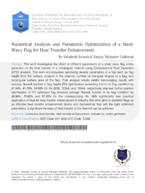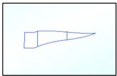FLAG HEIGHT (FH) OPTIMIZATION ### a) Representation of FH and CFD Simulations Figure 1 represents flag height (FH) which is varied to find the optimum height of RTTF from the plate. Shape-optimized RTTF and its arrangement in the channel by Swadesh Suman et al. [37] is used for FH optimization. The initial height of RTTF from the plate is $2.5 \, \text{mm}$. FH is varied from $0.5 \, \text{mm}$ to $5 \, \text{mm}$, increasing it by $0.5 \, \text{mm}$ from $0.5 \, \text{mm}$ to $3 \, \text{mm}$ and by $1 \, \text{mm}$ from $3 \, \text{mm}$ to $5 \, \text{mm}$. 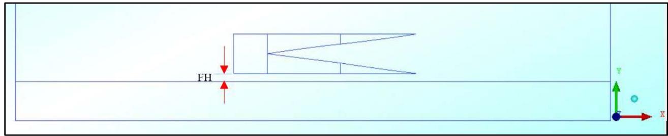 Figure 1: Representation of Flag Height (FH) 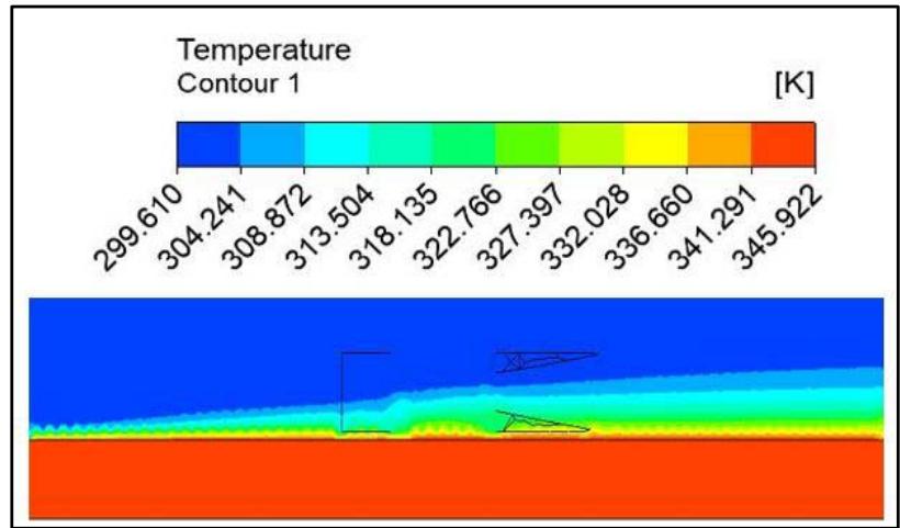 Figure 2a and 2b show the thermal boundary layer formed in the case of FH 1 mm and FH 2 mm. The temperature contour in each case shows the difference in temperature. Figure 2a): FH = 1 mm  Figure 2b): FH = 2 mm Figure 2: Thermal Boundary Layer at Different Flag Height ### b) Procedure followed during Calculations The procedure followed during the calculations is same as that used by Swadesh Suman et al. [37]. Fig 3 shows the lines plotted along the length of the channel and an average temperature is obtained for each line. The well distributed lines along the channel's height gives good idea of the average temperature of air at channel's outlet. 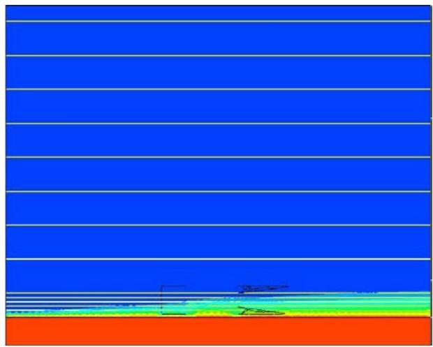 Figure 3: Lines Plotted along the Length of the Channel Following procedure is then followed to find out the average Nusselt number in each case:- Step 1: Mass flow rate $(\dot{M}) = \rho \times A_{c} \times V$ (5) Step 2: Temperature change in fluid $(T_{d}) = T_{o} - T_{i}$ (6) Step 3: Heat carried away by the fluid $(Q) = \dot{M} \times C_p \times T_d$ (7) Step 4: Average temperature difference between surface and fluid $(T_{a}) = T_{w} - T_{f}$ (8) Step 5: Average heat transfer coefficient $(h) = \frac{Q}{A_s \times T_a}$ (9) Step 6: Nusselt no $(Nu) = \frac{h\times D_h}{k}$ (10) Step 7:Reynolds no $(Re) = \frac{\rho\times V\times D_h}{\mu}$ (11) ### c) Results and Discussion Table 2 shows the Nusselt number for each flag height at different velocity conditions. The highest $Nu$ is achieved at a flag height equal to $1\mathrm{\;{mm}}$ for each velocity condition and it increases significantly by ${10.06}\%$, 7.28%, and 7.55% when compared with $Nu$ values for flag height of ${1.5}\mathrm{\;{mm}}$ and exceeds that in no flag condition by 41.84%, 47.79%, 54.68% for Re 8236, 12354 and 18344,respectively. $Nu$ values at each different velocity condition shoot up with the decrease in FH up to 1 mm. At FH $0.5 \mathrm{~mm}, N u$ values diminishes significantly by $11.1\%$, $9.3\%$, and $8.5\%$ than that of FH 1 mm for Re 8236, 12354, and 18344, respectively. The same has been depicted in fig 4 which presents the graph between $Nu$ and $Re$. Table 2: Nusselt Number at Different Flag Heights <table><tr><td>Velocity (m/s)</td><td>Nu</td><td>Re</td></tr><tr><td colspan="3">No flag condition</td></tr><tr><td>1.1</td><td>239</td><td>8236</td></tr><tr><td>1.65</td><td>249</td><td>12354</td></tr><tr><td>2.45</td><td>267</td><td>18344</td></tr><tr><td colspan="3">FH 0.5 mm</td></tr><tr><td>1.1</td><td>301</td><td>8236</td></tr><tr><td>1.65</td><td>334</td><td>12354</td></tr><tr><td>2.45</td><td>380</td><td>18344</td></tr><tr><td colspan="3">FH 1 mm</td></tr><tr><td>1.1</td><td>339</td><td>8236</td></tr><tr><td>1.65</td><td>368</td><td>12354</td></tr><tr><td>2.45</td><td>413</td><td>18344</td></tr><tr><td colspan="3">FH 1.5 mm</td></tr><tr><td>1.1</td><td>308</td><td>8236</td></tr><tr><td>1.65</td><td>343</td><td>12354</td></tr><tr><td>2.45</td><td>384</td><td>18344</td></tr><tr><td colspan="3">FH 2 mm</td></tr><tr><td>1.1</td><td>299</td><td>8236</td></tr><tr><td>1.65</td><td>312</td><td>12354</td></tr><tr><td>2.45</td><td>348</td><td>18344</td></tr><tr><td colspan="3">FH 2.5 mm</td></tr><tr><td>1.1</td><td>288</td><td>8236</td></tr><tr><td>1.65</td><td>301</td><td>12354</td></tr><tr><td>2.45</td><td>324</td><td>18344</td></tr><tr><td colspan="3">FH 3 mm</td></tr><tr><td>1.1</td><td>278</td><td>8236</td></tr><tr><td>1.65</td><td>294</td><td>12354</td></tr><tr><td>2.45</td><td>322</td><td>18344</td></tr><tr><td colspan="3">FH 4 mm</td></tr><tr><td>1.1</td><td>274</td><td>8236</td></tr><tr><td>1.65</td><td>291</td><td>12354</td></tr><tr><td>2.45</td><td>319</td><td>18344</td></tr><tr><td colspan="3">FH 5 mm</td></tr><tr><td>1.1</td><td>272</td><td>8236</td></tr><tr><td>1.65</td><td>287</td><td>12354</td></tr><tr><td>2.45</td><td>314</td><td>18344</td></tr></table> 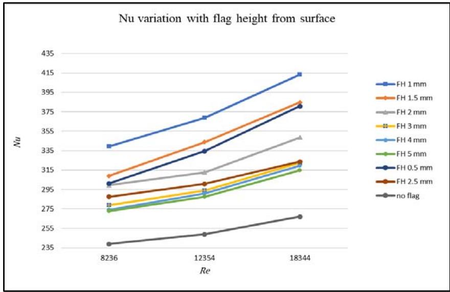 Figure 4: Average Nusselt Number vs Reynolds Number for Different Flag Heights ## IV. OPTIMIZATION OF POSITION OF FLAG IN CHANNEL ### a) Representation of Position of the Flag RTTF with FH 1 mm is used for the optimization of the position of the flag. Figure 5 represents the position of the flag from the inlet which is varied to find the optimum position of RTTF from the inlet. The initial position of RTTF from the inlet is $55 \mathrm{~mm}$. The position from the inlet is varied from $15 \mathrm{~mm}$ to $65 \mathrm{~mm}$, increasing it by $10 \mathrm{~mm}$ in each step. 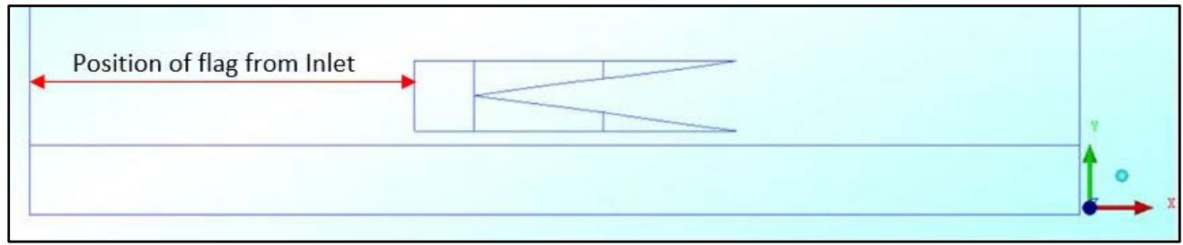 Figure 5: Representation of Position of Flag from inlet ### b) Procedure followed during Calculations The procedure followed for the calculation of $Nu$ is the same as that of Flag height optimization. ### c) Results and Discussion Table 3 shows the Nusselt number for the position of the flag at different velocity conditions. The highest $Nu$ is achieved at a flag position equal to $35\mathrm{mm}$ for each velocity condition. $Nu$ at flag position $35\mathrm{mm}$ is greater than that at flag position $25\mathrm{mm}$ by $2.63\%$, $6.78\%$, $10.13\%$, and by $2.03\%$, $8.97\%$, $12.10\%$ for Re 8236, 12354, 18344 respectively when compared with $N_u$ values for flag position $45 \mathrm{~mm}$. Whereas it exceeds $N_u$ in no flag condition by $46.86\%$, $70.68\%$, and $87.26\%$ for the corresponding Re. In each case, the percentage rise in $N_u$ increases with an increase in the velocity of air in the channel. $N_u$ values at each different velocity condition shoot up with the decrease in flag positions from $65 \mathrm{~mm}$ up to $35 \mathrm{~mm}$ and afterward, it diminishes till the flag position is $15 \mathrm{~mm}$. The same has been depicted in fig 6 which presents the graph between $N_u$ and Re. Table 3: Nusselt number at different flag positions <table><tr><td>Velocity (m/s)</td><td>Nu</td><td>Re</td></tr><tr><td colspan="3">No flag condition</td></tr><tr><td>1.1</td><td>239</td><td>8236</td></tr><tr><td>1.65</td><td>249</td><td>12354</td></tr><tr><td>2.45</td><td>267</td><td>18344</td></tr><tr><td colspan="3">Position of flag = 15 mm</td></tr><tr><td>1.1</td><td>340</td><td>8236</td></tr><tr><td>1.65</td><td>372</td><td>12354</td></tr><tr><td>2.45</td><td>438</td><td>18344</td></tr><tr><td colspan="3">Position of flag = 25 mm</td></tr><tr><td>1.1</td><td>342</td><td>8236</td></tr><tr><td>1.65</td><td>398</td><td>12354</td></tr><tr><td>2.45</td><td>454</td><td>18344</td></tr><tr><td colspan="3">Position of flag = 35 mm</td></tr><tr><td>1.1</td><td>351</td><td>8236</td></tr><tr><td>1.65</td><td>425</td><td>12354</td></tr><tr><td>2.45</td><td>500</td><td>18344</td></tr><tr><td colspan="3">Position of flag = 45 mm</td></tr><tr><td>1.1</td><td>344</td><td>8236</td></tr><tr><td>1.65</td><td>390</td><td>12354</td></tr><tr><td>2.45</td><td>446</td><td>18344</td></tr><tr><td colspan="3">Position of flag = 55 mm</td></tr><tr><td>1.1</td><td>339</td><td>8236</td></tr><tr><td>1.65</td><td>368</td><td>12354</td></tr><tr><td>2.45</td><td>413</td><td>18344</td></tr><tr><td colspan="3">Position of flag = 65 mm</td></tr><tr><td>1.1</td><td>268</td><td>8236</td></tr><tr><td>1.65</td><td>295</td><td>12354</td></tr><tr><td>2.45</td><td>319</td><td>18344</td></tr></table> 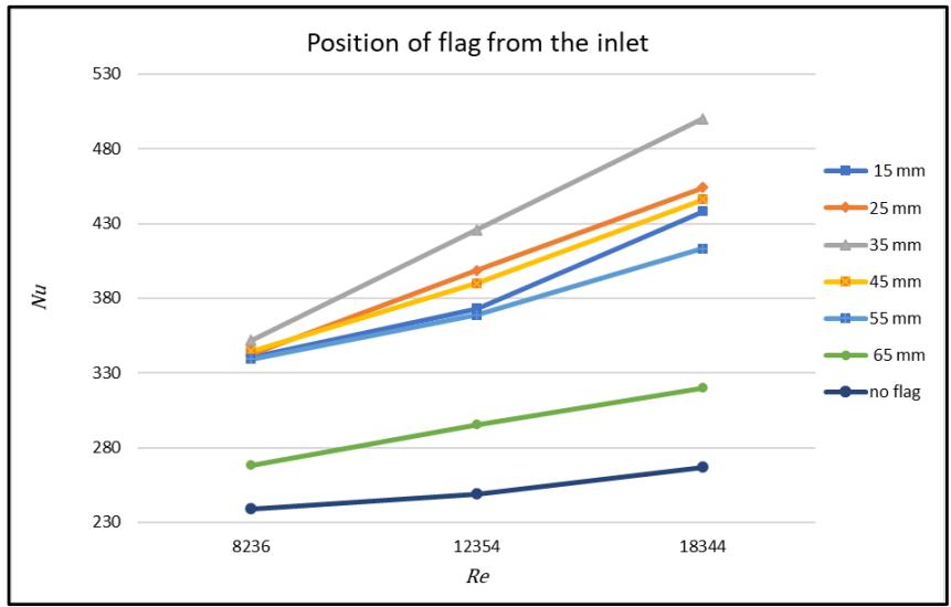 Figure 6: Average Nusselt number vs Reynolds number for different position of flag ## V. OPTIMIZATION OF NUMBER OF TRIANGULAR SHAPE IN RTTF ### a) Flag Geometries RTTF used for this stage has FH as $1\mathrm{mm}$ and position from the inlet as $35\mathrm{mm}$. In the investigation by Swadesh suman et al. [37], RTTF showed higher heat transfer than ROTF. So, to check the dependency of heat transfer on the number of triangular shapes, the number of triangular shapes is varied. Fig. 7 shows all five flag geometries. The total surface area of the triangular part of RTTF is kept constant while varying the number of triangular shapes. Fig 7 also incorporates the symbolic representation allotted to each flag with the different number of triangular shapes.  7a) Rectangular flag combined with one triangular flag (ROTF) 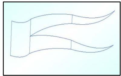 7b) Rectangular flag combined with two triangular flags (RTTF) 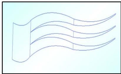 7c) Rectangular flag combined with three triangular flags (RTeTF) 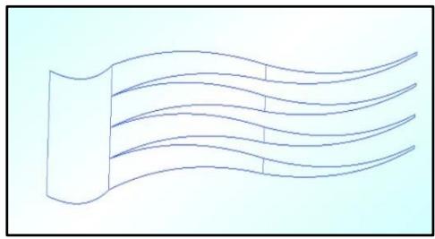 7d) Rectangular flag combined with four triangular flag (RFTF)  7e) Rectangular flag combined with five triangular flag (RFiTF) Figure 7: Flag geometries ### b) Procedure followed during Calculations The procedure followed for the calculation of $Nu$ is the same as that of Flag height optimization. ### c) Results and Discussion Table 4 shows the Nusselt number for flags with different triangular shapes at different velocity conditions. The highest $N_u$ is achieved for RTTF at each velocity condition. $N_u$ for RTTF is greater than RFiTF by 6.04%, 17.40%, 26.58% for Re 8236, 12354, 18344 respectively and by 8.33%, 18.71%, 31.57% for Re 8236, 12354, 18344 respectively when compared with $N_u$ values for RFTF. The percentage rise in $N_u$ of RTTF increases with an increase in velocity when compared to other flags. Fig 8 shows the graph between $N_u$ and $R e$ for each distinct flag. Table 4: Nusselt Number for Flags with Different Number of Triangular shapes <table><tr><td>Velocity (m/s)</td><td>Nu</td><td>Re</td></tr><tr><td colspan="3">No flag condition</td></tr><tr><td>1.1</td><td>239</td><td>8236</td></tr><tr><td>1.65</td><td>249</td><td>12354</td></tr><tr><td>2.45</td><td>267</td><td>18344</td></tr><tr><td colspan="3">ROTF</td></tr><tr><td>1.1</td><td>285</td><td>8236</td></tr><tr><td>1.65</td><td>308</td><td>12354</td></tr><tr><td>2.45</td><td>345</td><td>18344</td></tr><tr><td colspan="3">RTTF</td></tr><tr><td>1.1</td><td>351</td><td>8236</td></tr><tr><td>1.65</td><td>425</td><td>12354</td></tr><tr><td>2.45</td><td>500</td><td>18344</td></tr><tr><td colspan="3">RTeTF</td></tr><tr><td>1.1</td><td>281</td><td>8236</td></tr><tr><td>1.65</td><td>302</td><td>12354</td></tr><tr><td>2.45</td><td>341</td><td>18344</td></tr><tr><td colspan="3">RFTF</td></tr><tr><td>1.1</td><td>324</td><td>8236</td></tr><tr><td>1.65</td><td>358</td><td>12354</td></tr><tr><td>2.45</td><td>380</td><td>18344</td></tr><tr><td colspan="3">RFIETF</td></tr><tr><td>1.1</td><td>331</td><td>8236</td></tr><tr><td>1.65</td><td>362</td><td>12354</td></tr><tr><td>2.45</td><td>395</td><td>18344</td></tr></table> 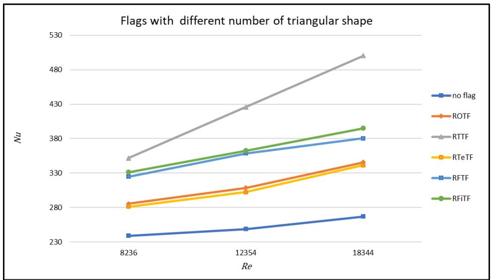 Figure 8: Average Nusselt number vs Reynolds number for different number of triangular shapes ## VI. OPTIMIZATION OF THE RECTANGULAR SURFACE (RS) AREA OF FLAG ### a) Problem Description RTTF has the highest heat transfer during the optimization process based on the number of triangular shapes. So, for the rectangular surface area optimization, RTTF is chosen. The surface area of the rectangular part in RTTF is $100\mathrm{mm}^2$. This area is varied from $50\mathrm{mm}^2$ to $150\mathrm{mm}^2$ with a step of $25\mathrm{mm}^2$. ### b) Procedure followed during Calculations The procedure followed for the calculation of $Nu$ is the same as that of Flag height optimization. ### c) Results and Discussion Table 5 shows the Nusselt number for flags with different RS areas at distinct velocity conditions. The highest $Nu$ is achieved for RTTF with RS area of 100 mm2 at each velocity condition. $Nu$ for RTTF with 100 mm2 is greater than that with 125 mm2 by 5.72%, 5.19%, 5.48% and that with 150 mm2 by 6.04%, 7.86%, 10.86% for Re 8236, 12354, 18344, respectively. Fig 9 shows the graph between $Nu$ and $Re$ for each distinct flag. Following fig 9, there is an increase in the $Nu$ with the increase in RS area from 50 mm2 to 100 mm2. At the RS area of 100 mm2, $Nu$ is the highest and afterward, it diminishes with an increase in RS area from 100 mm2 to 150 mm2. Table 5: Nusselt Number for Flags with Different Rectangular Area <table><tr><td>Velocity (m/s)</td><td>Nu</td><td>Re</td></tr><tr><td colspan="3">No flag condition</td></tr><tr><td>1.1</td><td>239</td><td>8236</td></tr><tr><td>1.65</td><td>249</td><td>12354</td></tr><tr><td>2.45</td><td>267</td><td>18344</td></tr><tr><td colspan="3">RS area = 50 mm2</td></tr><tr><td>1.1</td><td>309</td><td>8236</td></tr><tr><td>1.65</td><td>352</td><td>12354</td></tr><tr><td>2.45</td><td>395</td><td>18344</td></tr><tr><td colspan="3">RS area = 75 mm2</td></tr><tr><td>1.1</td><td>312</td><td>8236</td></tr><tr><td>1.65</td><td>356</td><td>12354</td></tr><tr><td>2.45</td><td>413</td><td>18344</td></tr><tr><td colspan="3">RS area = 100 mm2</td></tr><tr><td>1.1</td><td>351</td><td>8236</td></tr><tr><td>1.65</td><td>425</td><td>12354</td></tr><tr><td>2.45</td><td>500</td><td>18344</td></tr><tr><td colspan="3">RS area = 125 mm2</td></tr><tr><td>1.1</td><td>332</td><td>8236</td></tr><tr><td>1.65</td><td>404</td><td>12354</td></tr><tr><td>2.45</td><td>474</td><td>18344</td></tr><tr><td colspan="3">RS area = 150 mm2</td></tr><tr><td>1.1</td><td>331</td><td>8236</td></tr><tr><td>1.65</td><td>394</td><td>12354</td></tr><tr><td>2.45</td><td>451</td><td>18344</td></tr></table> 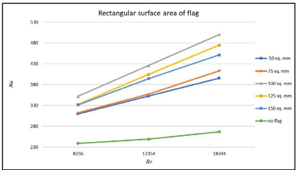 Figure 9: Average Nusselt Number vs Reynolds Number for Different Rectangular Surface Area of Flag ## VII. OPTIMAL PARAMETER SELECTION AND PERFORMANCE OPRIMIZATION This study is the extension of the investigation carried out by Swadesh Suman et al, [37]. RTTF which is the shape optimized flag according to Swadesh [37] is chosen for the optimization based on new parameters. RTTF's position in the channel is $55~\mathrm{mm}$ from the channel inlet and $2.5\mathrm{mm}$ from the surface. The position of the flag in the channel and flag height is chosen as the optimization parameters. Since RTTF is the combination of rectangular and two triangular shapes, therefore two other parameters namely the area of the rectangular part and the number of triangular shapes are also chosen as the optimization parameters. Similar to the method adopted by Swadesh [37], the overall optimization process is divided into four stages. For the first stage, RTTF of the shape optimization by Swadesh is considered and for the next stages, the optimized flag from the previous stage is considered. Table 6 shows the value of $Nu$ after each stage of parametric optimization. The% increase in $Nu$ in each case shoots up with the increase in the velocity of air in the channel. This can be seen in column 4 of Table 6. The highest increase in $Nu$ is observed during the optimization of the position of the flag in the channel. Table 6: Performance Optimization <table><tr><td colspan="4">Performance optimization</td></tr><tr><td>Velocity (m/s)</td><td>Nu</td><td>Re</td><td>% Increase in Nu/wrt no flag</td></tr><tr><td colspan="4">No flag condition</td></tr><tr><td>1.1</td><td>239</td><td>8236</td><td>0</td></tr><tr><td>1.65</td><td>249</td><td>12354</td><td>0</td></tr><tr><td>2.45</td><td>267</td><td>18344</td><td>0</td></tr><tr><td colspan="4">RTTF from Shape optimization (Swadesh [37])</td></tr><tr><td>1.1</td><td>288</td><td>8236</td><td>20.50</td></tr><tr><td>1.65</td><td>301</td><td>12354</td><td>20.88</td></tr><tr><td>2.45</td><td>324</td><td>18344</td><td>21.35</td></tr><tr><td colspan="4">After Flag height optimization</td></tr><tr><td>1.1</td><td>339</td><td>8236</td><td>41.84</td></tr><tr><td>1.65</td><td>368</td><td>12354</td><td>47.79</td></tr><tr><td>2.45</td><td>413</td><td>18344</td><td>54.68</td></tr><tr><td colspan="4">After Optimization of position of flag</td></tr><tr><td>1.1</td><td>351</td><td>8236</td><td>46.86</td></tr><tr><td>1.65</td><td>425</td><td>12354</td><td>70.68</td></tr><tr><td>2.45</td><td>500</td><td>18344</td><td>87.26</td></tr><tr><td colspan="4">After Optimization of number of triangular shapes</td></tr><tr><td>1.1</td><td>351</td><td>8236</td><td>46.86</td></tr><tr><td>1.65</td><td>425</td><td>12354</td><td>70.68</td></tr><tr><td>2.45</td><td>500</td><td>18344</td><td>87.26</td></tr><tr><td colspan="4">After Optimization of RS area</td></tr><tr><td>1.1</td><td>351</td><td>8236</td><td>46.86</td></tr><tr><td>1.65</td><td>425</td><td>12354</td><td>70.68</td></tr><tr><td>2.45</td><td>500</td><td>18344</td><td>87.26</td></tr></table> ## VIII. CONCLUSION This present numerical investigation focuses on the effect of different parameters of a static wavy flag vortex generator on heat transfer. These parameters are flag height from the surface, position in the channel, number of triangular shapes in a flag, and rectangular surface area of the flag. The method adopted for numerical investigation is Computational Fluid Dynamics (CFD) and the software used is ANSYS 2014.The ideal value of GSF for the geometry is selected as 2. The overall optimization process is divided into four stages with the first stage being the flag height optimization, the second stage is the position in the channel, the third stage is the number of triangular shapes and the fourth stage is the rectangular surface area of the flag. For each stage, the optimized flag from the previous stage is considered and for the first stage, shape optimized RTTF by Swadesh suman et al. [37] is considered. For the first stage, the highest $Nu$ is achieved at flag height equal to $1\mathrm{mm}$ for each velocity condition exceeding that in no flag condition by $41.84\%$ $47.79\%$ $54.68\%$ for Re 8236, 12354, and 18344, respectively. For the decrease in FH from $5\mathrm{mm}$ to $1\mathrm{mm}$, $Nu$ values showed an upward trend but with a further decrease in FH to $0.5\mathrm{mm}$ it diminished. For the second stage, the highest $Nu$ is achieved at the flag position equal to $35\mathrm{mm}$ and it exceeds that in no flag condition by $46.86\%$, $70.68\%$, and $87.26\%$ for Re 8236, 12354, 18344, respectively. A similar trend as the first stage in $Nu$ values is seen in the second one as well, it shoots up with the decrease in flag positions from $65\mathrm{mm}$ up to $35\mathrm{mm}$ and then decreases flag position to $15\mathrm{mm}$. In the third stage, RTTF with a flag height of $1\mathrm{mm}$ and flag position of $35\mathrm{mm}$ from the inlet has the highest $Nu$ when compared with flags with a different number of triangular shapes. For the fourth and final stage, RTTF with a rectangular area of $100\mathrm{mm}^2$ has the highest $Nu$ among the flags with the different rectangular areas. The $Nu$ increases with the increase in RS area from $50\mathrm{mm}^2$ to $100\mathrm{mm}^2$ and afterward, it diminishes with an increase in RS area from $100\mathrm{mm}^2$ to $150\mathrm{mm}^2$. Thus, from the results of this investigation, it can be deduced that with the right optimized parameters, a significant increase in heat transfer in the channel can be achieved.

Generating HTML Viewer...

References

39 Cites in Article
T Bergman,W Houf,F Incropera (2011). Effect of single scatter phase function distribution on radiative transfer in absorbing-scattering liquids.
Ralph Kristoffer,B Gallegos,N Rajnish,Sharma (2017). Flags as vortex generators for heat transfer enhancement: Gaps and challenges.
Mohsen Sheikholeslami,Mofid Gorji-Bandpy,Davood Ganji (2015). Review of heat transfer enhancement methods: Focus on passive methods using swirl flow devices.
H Ahmed,H Mohammed,M Yusoff (2012). An overview on heat transfer augmentation using vortex generators and nanofluids: Approaches and applications.
T Alam,R Saini,J Saini (2014). Use of turbulators for heat transfer augmentation in an air duct -A review.
Raj Amar,Anil Suri,Kumar,Maithani (2017). Convective Heat Transfer Enhancement Techniques of Heat Exchanger Tubes: A Review.
M Arulprakasajothi,U Chandrasekhar,K Elangovan,D Yuvarajan (2018). Influence of conical strip inserts in heat transfer enhancement under transition flow.
M Abeens,M Meikandan,Jaffar Sheriff,R Murunganadhan (2018). Experimental analysis of convective heat transfer on tubes using twisted tape inserts, louvered strip inserts and surface treated tube.
K Logesh,R Arunraj,S Govindan,M Thangaraj,G Yuvashree (2018). Numerical investigation on possibility of heat transfer enchancement using reduced weight fin configuration.
K Subramani,K Logesh,S Kolappan,S Karthik (2018). Experimental investigation on heat transfer characteristics of heat exchanger with bubble fin assistance.
Gareth Gilson,Stephen Pickering,David Hann,Chris Gerada (2013). Piezoelectric Fan Cooling: A Novel High Reliability Electric Machine Thermal Management Solution.
H Ma,S Liao,Y Li (2015). Study of multiple magnetic vibrating fins with a piezoelectric actuator.
H Ma,L Tan,Y Li (2014). Investigation of a multiple piezoelectric–magnetic fan system embedded in a heat sink.
Jae Bok,Lee,Sung Park,Boyoung Kim,Jaeha Ryu,Jin Hyung,Sung (2017). Heat transfer enhancement by flexible flags clamped vertically in a Poiseuille channel flow.
Jae Bok,Lee,Sung Park,Hyung Jinsung (2018). Heat transfer enhancement by asymmetrically clamped flexible flags clamped in a channel flow.
Zheng Li,Xianchen Xu,Kuojiang Li,Yangyang Chen,Guoliang Huang,Chung-Lung Chen,Chien-Hua Chen (2018). A flapping vortex generator for heat transfer enhancement in a rectangular airside fin.
Atul Kumar Soti,Rajneesh Bhardwaj,John Sheridan (2015). Flow-induced deformation of a flexible thin structure as manifestation of heat transfer enhancement.
Jaeha Ryu,Sung Park,Boyoung Kim,Hyung Sung (2015). Flapping dynamics of an inverted flag in a uniform flow.
Sung Park,Boyoung Kim,Cheong Chang,Jaeha Ryu,Hyung Sung (2016). Enhancement of heat transfer by a self-oscillating inverted flag in a Poiseuille channel flow.
F Herrault,P Hidalgo,C-H Ji,A Glezer,M Allen (2012). Cooling performance of micromachined self-oscillating reed actuators in heat transfer channels with integrated diagnostics.
Pablo Hidalgo,Ari Glezer (2011). Direct Actuation of Small-Scale Motions for Enhanced Heat Transfer in Heated Channels.
Pablo Hidalgo,Ari Glezer (2015). Small-Scale Vorticity Induced by a Self-Oscillating Fluttering Reed for Heat Transfer Augmentation in Air Cooled Heat Sinks.
Kourosh Shoele,Rajat Mittal (2014). Computational study of flow-induced vibration of a reed in a channel and effect on convective heat transfer.
A Bejan (1997). Advanced Engineering Thermodynamics, 2nd Edn Adrian Bejan, 1997 New York, Chichester, John Wiley & Sons ISBN 0-471-1-4880-6 £65.00.
Adrian Bejan,Sylvie Lorente (2008). Design with Constructal Theory.
Sylvie Lorente,Adrian Bejan (2019). Current trends in constructal law and evolutionary design.
Chen Lingen (2012). Progress in study on constructal theory and its applications.
Lingen Chen,Huijun Feng,Zhihui Xie,Fengrui Sun (2019). Progress of constructal theory in China over the past decade.
Adrian Bejan (1997). Constructal-theory network of conducting paths for cooling a heat generating volume.
Huijun Feng,Lingen Chen,Zhihui Xie (2017). Multi-disciplinary, multi-objective and multi-scale constructal optimizations for heat and mass transfer processes performed in Naval University of Engineering, a review.
Huijun Feng,Lingen Chen,Zhihui Xie (2018). Constructal optimizations for “+” shaped high conductivity channels based on entransy dissipation rate minimization.
Chen Lingen,Yang Aibo,Feng Huijun,Ge Yanlin,Xia Shaojun Constructal design progress for eight types of heat sinks.
Huijun Feng,Wanxu Qin,Lingen Chen,Cunguang Cai,Yanlin Ge,Shaojun Xia (2020). Power output, thermal efficiency and exergy-based ecological performance optimizations of an irreversible KCS-34 coupled to variable temperature heat reservoirs.
H Feng,L Chen,Z Xie,F Sun (2017). Constructal complex-objective optimization for tree-shaped hot water networks over a rectangular area using global optimization method.
Vineeth Swadesh Suman,Swati Uppada,Singh,Mahadev Sanjay,Gaikwad Numerical investigation and experimental validation of Shape amd Position optimization of a static wavy flag for heat transfer enhancement.
J Hinze (1975). Turbulence.
B E Launder,D Spalding (1974). The Numerical Computation of Turbulent Flows.
No ethics committee approval was required for this article type.
Data Availability
Not applicable for this article.
How to Cite This Article
Swadesh Suman. 2026. \u201cNumerical Analysis and Parametric Optimization of a Static Wavy Flag for Heat Transfer Enhancement\u201d. Global Journal of Research in Engineering - A : Mechanical & Mechanics GJRE-A Volume 22 (GJRE Volume 22 Issue A2).
Explore published articles in an immersive Augmented Reality environment. Our platform converts research papers into interactive 3D books, allowing readers to view and interact with content using AR and VR compatible devices.
Your published article is automatically converted into a realistic 3D book. Flip through pages and read research papers in a more engaging and interactive format.
Our website is actively being updated, and changes may occur frequently. Please clear your browser cache if needed. For feedback or error reporting, please email [email protected]
Thank you for connecting with us. We will respond to you shortly.