## I. INTRODUCTION A huge number of investigations have been performed in the last decade regarding the solar tracking systems. Among the aspects generally covered in these previous investigations are: the design model (mechanical structure), technology (sensors, actuators, microprocessors, and microcontrollers) algorithms (control schemes) and comparative efficiency (in what extent solar tracking systems are efficient). Based on experiments and experimentations, most of the previous works and investigations carried out, primarily aimed to determine the level of efficiency that could be expected by using a solar tracking system. Different results were concluded leading to discrepancies in terms of energy gain factor [1]. Based on theoretical geometrical considerations and some assumptions, [1] established the comparative energy efficiency of a dual axis solar tracking system to a static tilted cells array, as a function of latitude, day number and inclination angle (see Eq (19) and (21) as mentioned on page 453 of [1]) when the azimuthal deviation is set to zero. The study carried out by [1] did not take into account single axes solar trackers. Furthermore the main formulas obtained by [1] are valid when azimuthal deviation $(\lambda)$ is set to zero. Therefore extending the analysis on all cases of solar trackers and considering the non-zero azimuthal deviation are the motivations of this paper and define its major goals. For achieving the aforementioned goals, assumptions made by [1] are adopted and a straightforward vector analysis is used to compute ratios of daily solar energy received by systems (trackingers or static tilted photovoltaic cells). ## II. DUAL AXIS VERSUS STATIC TILTED PV CELL ARRAYS WITH A NON-ZERO AZIMUTHAL DEVIATION Let's recall that the vectors $\mathbf{ON}$ (Vector representing Normal irradiance to PV plane) and $\mathbf{OM}$ (Vector representing the incident solar irradiance) are expressed as follows [1]: $$ \boldsymbol {O M} \left( \begin{array}{c} I _ {m a x} \cos (\alpha) \sin (\gamma + \lambda) \\I _ {m a x} \cos (\alpha) \cos (\gamma + \lambda) \\I _ {m a x} \sin (\alpha) \end{array} \right); \boldsymbol {O N} \left( \begin{array}{c} 0 \\- I _ {m a x} \sin (\beta) \\I _ {m a x} \cos (\beta) \end{array} \right) $$ Where: - $\beta$ is the inclination angle of static tilted PV plane. 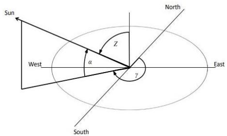- $\alpha$ (sun elevation angle) and $\gamma$ (sun azimuth angle) are as defined in appendix 1. - $\lambda$: azimuthal deviation (see appendix 2). The scalar product computation of $OM$ and $ON$, then leads to define the daily solar radiation captured by static tilted PV cells as: $$ R _ {s} = I _{max} \int_ {T _ {\text{rise}}} ^ {T _ {\text{set}}} | \cos \theta | d t \tag{1} $$ Where: - $T_{\text{rise}}$ and $T_{\text{set}}$ respectively denotes time of sun rise and that of sun set (See appendix1). - $\theta = (\mathbf{OM}, \mathbf{ON})$, i.e the angle between solar incident irradiance and the normal vector $\mathbf{ON}$ to the plane of PV cell arrays. - $R_{s} = R_{s}(\varphi,\beta,n,\lambda)$ The interval of integration $\left([T_{\text{rise}}, T_{\text{set}}]\right)$ is then subdivided in three intervals such that the sign of function $\cos \theta$ remains the same in each of them: $$ R _ {s} = I _ {\text{max}} \left[ \int_ {T _ {\text{rise}}} ^ {T _ {1}} I^c o s \theta | d t + \int_ {T _ {1}} ^ {T _ {2}} I^c o s \theta | d t + \int_ {T _ {2}} ^ {T _ {\text{set}}} I^c o s \theta | d t \right] \tag{2} $$ Where: - $T_{1}$ and $T_{2}$ respectively match the time when $\gamma = \pi - \lambda$; and $\gamma = \pi + \lambda$ (see appendix2). Let's define the (3x3) matrix S as follows: $$ \left( \begin{array}{l l} C _ {1} (g + T _ {0}) & \frac {1 2 C _ {2}}{\pi} \left[ \sin \left(\frac {\pi g}{1 2}\right) + \sin \left(\frac {\pi T _ {0}}{1 2}\right) \right] \\C _ {1} (h - g) & \frac {1 2 C _ {2}}{\pi} \left[ \sin \left(\frac {\pi h}{1 2}\right) - \sin \left(\frac {\pi g}{1 2}\right) \right] \\C _ {1} (T _ {0} - h) & \frac {1 2 C _ {2}}{\pi} \left[ \sin \left(\frac {\pi T _ {0}}{1 2}\right) - \sin \left(\frac {\pi h}{1 2}\right) \right] \end{array} - \frac {1 2 C _ {3}}{\pi} \left[ \cos \left(\frac {\pi g}{1 2}\right) - \cos \left(\frac {\pi T _ {0}}{1 2}\right) \right] \right) \tag {3} $$ Where: $$ C _ {1} = C _ {1} (\varphi , \beta , n, \lambda) = \sin \delta \left(\cos \beta \sin \varphi - \sin \beta \cos \varphi \cos \lambda\right) \tag {4} $$ $$ C _ {2} = C _ {2} (\varphi , \beta , n, \lambda) = \cos \delta \left(\cos \beta \cos \varphi + \sin \beta \sin \varphi \cos \lambda\right) \tag {5} $$ $$ C _ {3} = C _ {3} (\varphi , \beta , n, \lambda) = \sin \beta \cos \delta \sin \lambda $$ $$ T _ {0} = T _ {0} (\varphi , n) = \frac {1 2}{\pi} \cos^ {- 1} (- \tan \varphi \tan \delta) \tag {7} $$ $$ h = h (\varphi , n, \lambda) = \frac {2 4}{\pi} \tan^ {- 1} \left[ \frac {\cot \lambda - \sqrt {\left(\cot \lambda\right) ^ {2} + \left(\sin \varphi\right) ^ {2} - \left(\cos \varphi\right) ^ {2} \left(\tan \delta\right) ^ {2}}}{\sin \varphi + \cos \varphi \tan \delta} \right] \tag {8} $$ $$ g = g (\varphi , n, \lambda) = \frac {2 4}{\pi} t a n ^ {- 1} \left[ \frac {- c o t \lambda + \sqrt {(c o t \lambda) ^ {2} + (s i n \varphi) ^ {2} - (c o s \varphi) ^ {2} (t a n \delta) ^ {2}}}{s i n \varphi + c o s \varphi t a n \delta} \right] \tag {9} $$ Computing (2) and using (3) yield: $$ R _ {m a x} = \left[ \frac {2 * T _ {0}}{\left| \sum_ {j = 1} ^ {3} S _ {1 j} \right| + \left| \sum_ {j = 1} ^ {3} S _ {2 j} \right| + \left| \sum_ {j = 1} ^ {3} S _ {3 j} \right|} \right] * R _ {s} \tag {10} $$ Where: - $R_{\text{max}}$ stands for daily energy captured by a dual axis solar tracker. - $R_{s}$ is the daily energy received by a static tilted PV plane. By setting: $$ K _ {D S} = \frac {2 * T _ {0}}{\left| \sum_ {j = 1} ^ {3} S _ {1 j} \right| + \left| \sum_ {j = 1} ^ {3} S _ {2 j} \right| + \left| \sum_ {j = 1} ^ {3} S _ {3 j} \right|} \tag {11} $$ Energy efficiency (gain factor) of dual axis to static PV cell arrays is then measured by: $$ \eta_ {D S} (\varphi , \beta , n, \lambda) = K _ {D S} (\varphi , \beta , n, \lambda) - 1 \tag {12} $$ In Southern Hemisphere variables $\varphi$ and $\beta$ should be replaced by their opposites i.e. by $-\varphi$ and $-\beta$ in all of the previous and next equations that involve these variables. It is worth noticing that tend $\lambda$ to zero leads to (21) of [1]: $$ \lim _ {\lambda \rightarrow 0} \eta_ {D S} (\varphi , \beta , n, \lambda) = \eta (\varphi , \beta , n) \tag {13} $$ ## III. DUAL AXIS TRACKING VERSUS SINGLE VERTICAL AXIS TRACKING (PERFORMING HORIZONTAL TRACKING) TILTED WITH A CERTAIN INCLINATION ANGLE Let's consider a single axis tracker that performs rotational movement around a vertical axis according the principle that its angular rotation is locked on solar azimuth $(\gamma)$. Furthermore the PV cells array fastened on the vertical axis are assumed to be tilted with a certain inclination angle (Figure1 and FigureA2.1 of appendix2). Let's $\mathbf{OP}$ be the normal vector to the PV plane of the tracker. As the system tracks azimuth angle $(\gamma)$ it is not relevant to consider a certain azimuthal deviation so that $\mathbf{OP}$ and $\mathbf{OM}$ are expressed as: 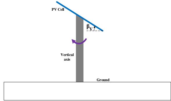 Figure 1: Single vertical axis tracker tilted $$ \boldsymbol {O M} \binom {I _ {\max } \cos (\alpha) \sin (\gamma)} {I _ {\max } \cos (\alpha) \cos (\gamma)}; \boldsymbol {O P} \binom {I _ {\max } \sin \left(\beta_ {V}\right) \sin (\gamma)} {I _ {\max } \sin \left(\beta_ {V}\right) \cos (\gamma)} \tag {14} $$ If $R_{v}$ denotes the total daily energy captured by the single vertical axis tracker, then (14) yields: $$ R _ {v} = \left(\int_ {T _ {\text{rise}}} ^ {T _ {\text{set}}} \sin \left(\beta_ {V}\right) \cos \alpha d t + \int_ {T _ {\text{rise}}} ^ {T _ {\text{set}}} \cos \left(\beta_ {V}\right) \sin \alpha d t\right) * I _{max} \tag{15} $$ To compute (15), power series expansion is used and the end result includes matrix (V) elements which are defined as follows (see appendix 2 for operation details): $$ V _ {1 1} = \left(1 - \frac {a ^ {2}}{2} - \frac {a ^ {4}}{4}\right) \left(1 - \cos \left(\frac {\pi T _ {0}}{1 2}\right)\right) \left(\frac {1 2 \sin \beta_ {V}}{\pi}\right) \tag {16} $$ $$ V _ {1 2} = - \frac{a b}{2} \left(1 + \frac{a ^ {2}}{2}\right) \left(1 - \left(\cos \left(\frac{\pi T _ {0}}{1 2}\right)\right) ^ {2}\right) \left(\frac{1 2 \sin \beta_ {V}}{\pi}\right) \tag{17} $$ $$ V _ {1 3} = - \frac{a ^ {2}}{6} \left(1 + \frac{a ^ {2}}{8} + b ^ {2}\right) \left(1 - \left(\cos \left(\frac{\pi T _ {0}}{1 2}\right)\right) ^ {3}\right) \left(\frac{1 2 \sin \beta_ {V}}{\pi}\right) \tag{18} $$ $$ V _ {2 1} = - \frac{a b}{8} \left(2 + \frac{a ^ {2}}{2}\right) \left(1 - \left(\cos \left(\frac{\pi T _ {0}}{1 2}\right)\right) ^ {4}\right) \left(\frac{1 2 \sin \beta_ {V}}{\pi}\right) \tag{19} $$ $$ V _ {2 2} = a \left(\cos \left(\beta_ {V}\right)\right) T _ {0} $$ $$ V _ {2 3} = \frac {1 2 b}{\pi} \left(\cos \beta_ {V}\right) \left(\sin \left(\frac {\pi T _ {0}}{1 2}\right)\right) \tag {21} $$ Where: $$ a = a (\varphi , n) = \sin \delta \sin \varphi $$ $$ b = b(\varphi , n) = \cos\delta\cos\varphi $$ It comes: $$ R_{max} = \frac{T_0}{\left| \sum_{i=1}^2 \sum_{j=1}^3 V_{ij} \right|} * R_v \tag{24} $$ We define $K_{DV}$ (Dual axis to Vertical axis) factor as: $$ K _ {D V} (\varphi , \beta_ {V}, n) = \frac {T _ {0}}{\left| \sum_ {i = 1} ^ {2} \sum_ {j = 1} ^ {3} V _ {i j} \right|} \tag {25} $$ The energy efficiency of dual axis tracking system to single vertical axis tracking system with a tilt angle $\beta_{V}$ is measured by: $$ \eta_ {D V} (\varphi , \beta_ {V}, n) = K _ {D V} (\varphi , \beta_ {V}, n) - 1 \tag {26} $$ ## IV. DUAL AXIS TRACKING VERSUS SINGLE HORIZONTAL AXIS TRACKING (PERFORMING VERTICAL TRACKING) TILTED WITH A CERTAIN INCLINATION ANGLE The horizontal tracker is assumed to rotate according a certain angle locked with solar elevation angle $(\alpha)$. Accordingly, for the first half of day length, two limit positions are defined: - $\alpha = \alpha_{1} = 0$, at time of sunrise ( $T_{rise}$ ). - $\alpha = \alpha_{2}$ (the highest elevation angle) at local noon. Where: $$ \alpha_ {2} = \sin^ {- 1} (a + b) \tag{27} $$ The general case deals with the single horizontal tracker with azimuthal deviation $(\lambda_{H})$ that might be comprised between $0^{\circ}$ to $90^{\circ}$ (from south to East, counterclockwise, in northern hemisphere; or from North to West, counterclockwise, in southern hemisphere) or between 0 to $-90^{\circ}$ (from south to West, clockwise, in northern hemisphere; or from North to East clockwise in southern hemisphere). Let's $\mathbf{OQ}$ be the normal vector to the PV plane of the tracker (Figure2). Vectors $\mathbf{OQ}$ and $\mathbf{OM}$ (Vector representing the incident solar irradiance) are expressed as follows: $$ \boldsymbol {O M} \binom {I _ {\max } \cos (\alpha) \sin (\gamma + \lambda)} {I _ {\max } \cos (\alpha) \cos (\gamma + \lambda)}; \boldsymbol {O Q} \binom {I _ {\max } \cos \alpha} {- I _ {\max } \sin (\beta_ {H}) \sin \alpha} \tag {28} $$ 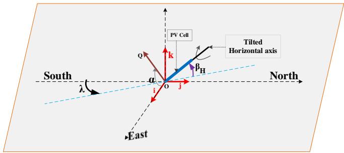 Figure 2: Single horizontal axis tracker tilted The total daily energy $(R_{H})$ captured by the single horizontal axis tracker, is given by: $$ R _ {H} = 2 \int_ {T _ {\text{rise}}} ^ {1 2} \cos (\boldsymbol{O M}, \boldsymbol{O N}) d t \tag{29} $$ The (3x3) matrix $H$ is introduced and defined by: $$ H _ {1 1} (\varphi , \beta_ {H}, n, \lambda) = \frac {- 6 \cos \lambda [ \alpha_ {2} + (a + b) \cos \alpha_ {2} ]}{\pi \cos \varphi} \tag {30} $$ $$ H _ {1 2} (\varphi , \beta_ {H}, n, \lambda) = d \left[ X _ {1} \left(1 - \cos \frac {\pi T _ {0}}{1 2}\right) + \frac {X _ {2}}{2} \left(1 - \cos^ {2} \frac {\pi T _ {0}}{1 2}\right) \right] \tag {31} $$ $$ H _ {1 3} (\varphi , \beta_ {H}, n, \lambda) = d \left[ \frac {X _ {3}}{3} \left(1 - \cos^ {3} \frac {\pi T _ {0}}{1 2}\right) + \frac {X _ {4}}{4} \left(1 - \cos^ {4} \frac {\pi T _ {0}}{1 2}\right) \right] \tag {32} $$ $$ H _ {2 1} \left(\varphi , \beta_ {H}, n, \lambda\right) = e \left[ \frac{X _ {1}}{2} \left(1 - \cos^ {2} \frac{\pi T _ {0}}{1 2}\right) + \frac{X _ {2}}{3} \left(1 - \cos^ {3} \frac{\pi T _ {0}}{1 2}\right) \right] \tag{33} $$ $$ H _ {2 2} \left(\varphi , \beta_ {H}, n, \lambda\right) = e \left[ \frac {X _ {3}}{4} \left(1 - \cos^ {4} \frac {\pi T _ {0}}{1 2}\right) + \frac {X _ {4}}{5} \left(1 - \cos^ {5} \frac {\pi T _ {0}}{1 2}\right) \right] \tag {34} $$ $$ H _ {2 3} \left(\varphi , \beta_ {H}, n, \lambda\right) = \left(p _ {1} + \frac{p _ {3}}{2}\right) T _ {0} + \frac{3 P _ {3}}{\pi} \sin \left(\frac{\pi T _ {0}}{6}\right) + \frac{1 2 P _ {2}}{\pi} \sin \left(\frac{\pi T _ {0}}{1 2}\right) \tag{35} $$ $$ H _ {3 1} \left(\varphi , \beta_ {H}, n, \lambda\right) = \left(- \frac{6}{\pi}\right) \left(2 q _ {1} + q _ {2}\right) + \frac{1 2 q _ {1}}{\pi} \cos \left(\frac{\pi T _ {0}}{1 2}\right) + \frac{6 q _ {2}}{\pi} \cos \left(\frac{\pi T _ {0}}{6}\right) \tag{36} $$ $$ H _ {3 2} (\varphi , \beta_ {H}, n, \lambda) = \cos \beta_ {H} \left[ \left(a ^ {2} + \frac {b ^ {2}}{2}\right) T _ {0} + \frac {2 4 a b}{\pi} \sin \left(\frac {\pi T _ {0}}{1 2}\right) + \frac {3 b ^ {2}}{\pi} \sin \left(\frac {\pi T _ {0}}{6}\right) \right] \tag {37} $$ $$ H _ {3 3} (\varphi , \beta_ {H}, n, \lambda) = d \frac {X _ {5}}{5} \Big (1 - c o s ^ {5} \frac {\pi T _ {0}}{1 2} \Big) + e \frac {X _ {5}}{6} \Big (1 - c o s ^ {6} \frac {\pi T _ {0}}{1 2} \Big) $$ Where: $$ X _ {1} = X _ {1} (\varphi , n) = 1 - \frac {a ^ {2}}{2} - \frac {a ^ {4}}{8} \tag {38} $$ $$ X _ {2} = X _ {2} (\varphi , n) = - a b \left(1 + \frac {a ^ {2}}{2}\right) \tag {39} $$ $$ X _ {3} = X _ {3} (\varphi , n) = - \frac {a ^ {2}}{2} \left(1 + \frac {a ^ {2}}{8} + b ^ {2}\right) \tag {40} $$ $$ X _ {4} = X _ {4} (\varphi , n) = - \frac {a b}{2} \left(2 + \frac {a ^ {2}}{2}\right) \tag {41} $$ $$ X _ {5} = X _ {5} (\varphi , n) = - \frac {a ^ {2}}{4} \left(b ^ {2} + \frac {3 a ^ {2}}{1 6} + \frac {5}{4}\right) \tag {42} $$ $$ p _ {1} = p _ {1} \left(\varphi , \beta_ {H} , n , \lambda\right) = - a \sin \beta_ {H} \cos \lambda \sin \delta \cos \varphi $$ $$ p_{2} = p_{2}(\varphi,\beta_{H},n,\lambda) = - (\sin\beta_{H}\cos\lambda)(b\sin\delta\cos\varphi - a\cos\delta\sin\varphi) $$ $$ p _ {3} = p _ {3} \left(\varphi , \beta_ {H}, n, \lambda\right) = b \sin \beta_ {H} \cos \lambda \cos \delta \sin \varphi $$ $$ d = d(\varphi, n, \lambda) = \frac{12}{\pi} \sin\lambda\sin\delta\cos\varphi $$ $$ e = e(\varphi, n, \lambda) = -\frac{12}{\pi} \sin\lambda\cos\delta\sin\varphi $$ $a = a(\varphi,n)$ and $b = b(\varphi,n)$ are respectively defined by (22) and (23). The total daily energy captured by a dual tracker compared to that of single horizontal axis is then expressed as: $$ R _ {m a x} = \frac {T _ {0}}{\left| \sum_ {i = 1} ^ {3} \sum_ {j = 1} ^ {3} H _ {i j} \right|} * R _ {H} \tag {48} $$ Setting: $$ K _ {D H} (\varphi , \beta_ {H}, n, \lambda) = \frac {T _ {0}}{\left| \sum_ {i = 1} ^ {3} \sum_ {j = 1} ^ {3} H _ {i j} \right|} \tag {49} $$ Allows to define the energy efficiency factor of a dual axis tracker compared to a single horizontal axis as: $$ \eta_ {D H} (\varphi , \beta_ {H}, n, \lambda) = K _ {D H} (\varphi , \beta_ {H}, n, \lambda) - 1 \tag {50} $$ ## V. SINGLE VERTICAL AXIS TRACKING (PERFORMING HORIZONTAL TRACKING) VERSUS STATIC TILTED PV CELL ARRAYS The energy efficiency factor of a single vertical axis tracker compared to static PV arrays is established by inference, using (10), (11), (24) and (25): $$ \eta_ {V S} (\varphi , \beta , \beta_ {V}, n, \lambda) = \frac {K _ {D S} (\varphi , \beta , n , \lambda)}{K _ {D V} (\varphi , \beta_ {V} , n)} - 1 \tag {51} $$ ## VI. SINGLE HORIZONTAL AXIS TRACKING (PERFORMING VERTICAL TRACKING) VERSUS STATIC TILTED PV CELL ARRAYS By inference, using (10), (11), (48) and (49), the energy efficiency factor of a single horizontal axis compared to static PV arrays, is established: $$ \eta_ {H S} (\varphi , \beta , \beta_ {H}, n, \lambda , \lambda_ {H}) = \frac {K _ {D S} (\varphi , \beta , n , \lambda)}{K _ {D H} (\varphi , \beta_ {H} , n , \lambda_ {H})} - 1 \tag {52} $$ Where: $\lambda_{H}$ denotes azimuthal deviation of single horizontal axis tracker; and $\lambda$ that of static PV arrays. ## VII. RESULTS AND DISCUSSION Three Matlab scripts (see appendix 3) were written for performing numerical computations that emphasize minimum efficiency values of dual axis tracking compared to single axes tracking and static (with azimuthal deviation) PV cell arrays. Three major results derived from computations: 1) The numerical results of Script#1 show that a static tilted PV array with a non-zero azimuthal deviation is less efficient than one without azimuthal deviation. In fact, a non-zero azimuthal deviation of static tilted PV array leads to a yearly tilt angle which is not optimal. That confirms the fact that the tilt angle of static PV array should be, rigorously, either due South (in Northern Hemisphere) or due North (in Southern Hemisphere) for an increased energy efficiency. 2) Numerical results of Script#2 and Script#3, clearly show that a single vertical axis tracking (which performs horizontal tracking of sun position) is generally more efficient than a single horizontal axis tracking system (which performs vertical tracking of sun position). That confirms the conclusion of [2] regarding the efficiency comparison of single vertical axis and single horizontal axis tracking systems. 3) Script#3 numerical results show that increasing azimuthal deviation of a single horizontal axis tracking system (that performs vertical tracking of sun position) leads to increase its efficiency. ## VIII. CONCLUSION The study carried out in this paper, formerly, established the general energy efficiency equations of both solar tracking systems (dual and single) and static tilted PV arrays. The equations were expressed as multivariable functions of latitude, inclination angle, day number and azimuthal deviation. The study concluded that single vertical axis tracking, that performs horizontal tracking of sun position, is more efficient than single horizontal axis which performs vertical tracking of sun position. However it remains to decide, according the earth location, which slope angle should be optimal for a single vertical axis solar tracking system. ### ACKNOWLEDGMENTS The author thanks Dr. Maliki Guindo, Power Systems Professor at National School of Engineers and Mr. Abibaye Traoré for their constant advices and support. A special thank to Dr. Hamadoun Touré for his mentorship. #### APPENDIX #### Appendix 1 The earth follows a complex motion that consists of the daily motion and the annual motion. The daily motion causes the sun to appear in the east to west direction over the earth whereas the annual motion causes the sun to tilt at a particular angle while moving along east to west direction. Declination angle $\delta$ (Figure A.1) accounts for annual motion; azimuth angle $\gamma$ (Figure A.2) and elevation (or altitude) angle $\alpha$ (Figure A.2) characterize the daily motion. 1) Sun declination angle$\delta$is defined to be that angle made between a ray of the sun, when extended to the center of the earth, and the equatorial plane. 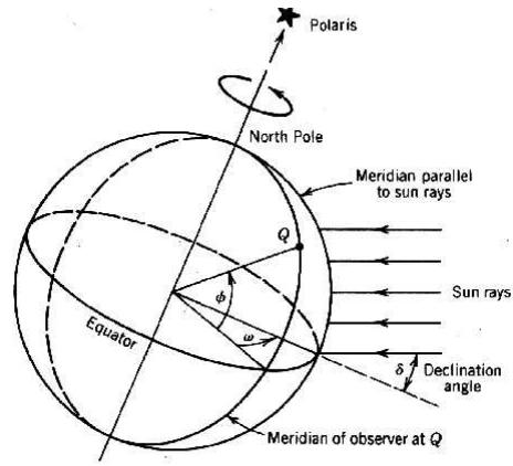$$ \delta = 23.45\sin\left[360\left(\frac{284+n}{365}\right)\right] $$ $\delta$: Declination angle in degrees $n$: day number ( $n = 1$ at the first of January)  Figure A1.1 2) Solar elevation (altitude) angle $\alpha$ (Fig A1.2) is the angle between the projection of the sun's rays on the horizontal plane and the direction on the sun's rays. $$ \alpha = \sin^ {- 1} (\sin \delta \sin \varphi + \cos \delta \cos \varphi \cos \omega) \tag {A1.2} $$ Where: $\delta$: Declination angle $\varphi$: Observer's latitude $\omega$: hour angle  Figure A1.2 3) Hour angle $(\omega)$ is the angular displacement from east to west of the local meridian due to rotation of the earth on its axis at $15^{\circ}$ per hour: $$ \omega = 15(t - 12)\tag{A1.3} $$ 4) Latitude $\varphi$ (Fig A.1) of a location on the earth is the angle between the line joining that location to the center of the earth and the equatorial plane. 5) Zenith angle Z (Fig A.2) is the complement of altitude angle: $$ Z = 9 0 ^ {\circ} - \alpha \tag{A1.4} $$ 6) Azimuth angle$\gamma$is the local angle between the direction of due north and that of the perpendicular projection of the sun down onto the horizon line, measured clockwise. The following relation relates the sun azimuth angle and its elevation angle: $$ \cos \alpha . \cos \gamma = \sin \delta \cos \varphi - \cos \delta \sin \varphi \cos \omega \tag {A1.5} $$ It can also be shown that: $$ \cos\alpha\cdot\sin\gamma=\cos\delta\sin\omega $$ 7) Latitude $\varphi$ (denoted by $\phi$ on Figure A1.1) of a location on the earth is the angle between the line joining that location to the center of the earth and the equatorial plane. $$ T _ {r i s e} = 1 2 - T _ {0} \tag {A1.7} $$ $$ T _ {s e t} = 1 2 + T _ {0} \tag {A1.8} $$ With $$ T _ {0} = \frac {1 2}{\pi} \cos^ {- 1} (- \tan \varphi . \tan \delta) \tag {A1.9} $$ #### Appendix 2 #### 1) Dividing [A1.5] by [A1.6] yields: $$ \cot \gamma = \frac {1}{2} \cos \varphi \tan \delta \frac {1}{\sin \omega} - \sin \varphi \frac {\cos \omega}{\sin \omega} \tag {A2.1} $$ Using trigonometric transformations, [A2.1] gives a second order polynomial equation: $$ \frac {1}{2} \left(\cos \varphi \tan \delta + \sin \varphi\right) X ^ {2} + (- \cot \gamma) X + \frac {1}{2} \left(\cos \varphi \tan \delta - \sin \varphi\right) = 0 \tag {A2.2} $$ With: $$ X = \tan {\frac {\omega}{2}} \qquad [ \mathrm {A 2 . 3} ] $$ The solutions which derive from [A2.2] are defined as: $$ \left\{ \begin{array}{l} X _ {1} = \frac {\cot \gamma - \sqrt {\cot^ {2} \gamma + \sin^ {2} \varphi - \cos^ {2} \varphi \tan^ {2} \delta}}{\cos \varphi \tan \delta + \sin \varphi} \\ X _ {2} = \frac {\cot \gamma + \sqrt {\cot^ {2} \gamma + \sin^ {2} \varphi - \cos^ {2} \varphi \tan^ {2} \delta}}{\cos \varphi \tan \delta + \sin \varphi} \end{array} \right. \tag {A2.4} $$ Assuming that $\gamma = \pi -\lambda$ at time $t = t_1$ and $\gamma = \pi +\lambda$ at time $t = t_2$ involves the following condition: $$ 0 \leq T _ {r} \leq T _ {1} \leq 1 2 \leq T _ {2} \leq T _ {\text {s e t}} \tag {A2.5} $$ [A2.4] and [A2.5] allow to define: $$ \left\{ \begin{array}{l} T _ {1} (\varphi , n, \lambda) = \frac {24}{\pi} \tan^{-1} \left(\frac {\sqrt {\cot^{2} \lambda + \sin^{2} \varphi - \cos^{2} \varphi \tan^{2} \delta} - \cot \lambda}{\cos \varphi \tan \delta + \sin \varphi}\right) + 12 \\ T _ {2} (\varphi , n, \lambda) = \frac {24}{\pi} \tan^{-1} \left(\frac {\cot \lambda - \sqrt {\cot^{2} \lambda + \sin^{2} \varphi - \cos^{2} \varphi \tan^{2} \delta}}{\cos \varphi \tan \delta + \sin \varphi}\right) + 12 \end{array} \right. \tag {A2.6} $$ If we set: $$ \left\{ \begin{array}{l} g (\varphi , n, \lambda) = \frac {24}{\pi} \tan^{-1} \left(\frac {\sqrt {\cot^{2} \lambda + \sin^{2} \varphi - \cos^{2} \varphi \tan^{2} \delta} - \cot \lambda}{\cos \varphi \tan \delta + \sin \varphi}\right) \\ h (\varphi , n, \lambda) = \frac {24}{\pi} \tan^{-1} \left(\frac {\cot \lambda - \sqrt {\cot^{2} \lambda + \sin^{2} \varphi - \cos^{2} \varphi \tan^{2} \delta}}{\cos \varphi \tan \delta + \sin \varphi}\right) \end{array} \right. \tag {A2.7} $$ Then: $$ \left. \int T _ {1} (\varphi , n, \lambda) = g (\varphi , n, \lambda) + 1 2 \right. \tag {A2.8} $$ $$ \left\lfloor T _ {2} (\varphi , n, \lambda) = h (\varphi , n, \lambda) + 1 2 \right. $$ 2) The inclination direction for a static PV array or a single horizontal axis tracking system is assumed to be North-South facing in Northern Hemisphere and South-North facing in Southern Hemisphere, to ensure better energy efficiency. However, the present study assumes some minor or major deviations around the North-South direction or the South-North direction, in order to rigorously determine whether such deviations, called azimuthal, may either decrease or increase the overall energy efficiency of PV systems. In this paper, azimuthal deviation is positively counted when it is South due East, counterclockwise in Northern Hemisphere or North due West, counterclockwise, in Southern Hemisphere; and negatively when it is South due West, clockwise, in Northern Hemisphere, or North due East, clockwise, in Southern hemisphere. The values of azimuthal deviation are considered in the following interval: $$ \left\{ \begin{array}{l} - 9 0 ^ {\circ} \leq \lambda \leq + 9 0 ^ {\circ} \\ - 9 0 ^ {\circ} \leq \lambda_{H} \leq + 9 0 ^ {\circ} \end{array} \right. \tag {A2.9} $$ Where $\lambda$ sets for static PV system azimuthal deviation and $\lambda_{H}$ for that of PV single horizontal axis tracking system (performing vertical tracking of sun position). 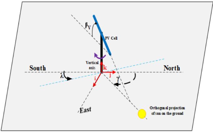3) The principle of horizontal tracking by a single vertical axis tracker is schematized below:  Figure A2.1: Single vertical axis tracking system #### 4) Let's recall (15): $$ R _ {v} = \left(\int_ {T _ {\text {r i s e}}} ^ {T _ {\text {s e t}}} \sin \left(\beta_ {V}\right) \cos \alpha d t + \int_ {T _ {\text {r i s e}}} ^ {T _ {\text {s e t}}} \cos \left(\beta_ {V}\right) \sin \alpha d t\right) * I _ {\max } \tag {A2.10} $$ That can be rewritten as: $$ \frac {R _ {v}}{2 * I _ {\text {m a x}}} = \sin \left(\beta_ {V}\right) \int_ {T _ {\text {r i s e}}} ^ {1 2} \cos \alpha d t + \cos \left(\beta_ {V}\right) \int_ {T _ {\text {r i s e}}} ^ {1 2} \sin \alpha d t \tag {A2.11} $$ The right hand side of [A2.11] consists of two integral parts: $$ \left\{ \begin{array}{l} I _ {1} = \sin \left(\beta_ {V}\right) \int_ {T _ {\text {r i s e}}} ^ {1 2} \cos \alpha \, dt \\I _ {2} = \cos \left(\beta_ {V}\right) \int_ {T _ {\text {r i s e}}} ^ {1 2} \sin \alpha \, dt \end{array} \right. \tag{A2.12} $$ Otherwise, [A2.12] is equivalent to: $$ \left\{ \begin{array}{c} I _ {1} = \sin \left(\beta_ {V}\right) \int_ {T _ {\text {r i s e}}} ^ {1 2} \sqrt {1 - (a + b \cos \omega) ^ {2}} d t \\ I _ {2} = \cos \left(\beta_ {V}\right) \int_ {T _ {\text {r i s e}}} ^ {1 2} (a + b \cos \omega) d t \end{array} \right. \tag {A2.13} $$ Where $\omega$ is expressed by [A1.3] and rewritten as: $$ \omega = \frac {\pi}{1 2} (t - 1 2) \tag {A2.14} $$ To compute the first integral, $I_{1}$ let's make a change of variable by setting: $$ x = \cos \omega \tag {A2.15} $$ Then it comes: $$ I _ {1} = \frac {1 2}{\pi} \sin \left(\beta_ {V}\right) \int_ {x _ {0}} ^ {x _ {1}} \frac {\sqrt {1 - (a + b x) ^ {2}}}{\sqrt {1 - x ^ {2}}} d t \tag {A2.16} $$ Where $a$ and $b$ are respectively defined by (22) and (23). And as: $$ \left\{ \begin{array}{l} - 1 \leq a \leq 1 \\ - 1 \leq b \leq 1 \\ 0 \leq x \leq 1 \end{array} \right. \tag{A2.17} $$ The following power series expansion: $$ (1 + X) ^ {p} = 1 + p X + \frac {p (p - 1)}{2 !} X ^ {2} + \dots + \frac {p (p - 1) \dots (p - n + 1)}{n !} X ^ {n} + \dots \tag {A2.18} $$ Is used to compute $I_{1}$. Afterward, the second integral, $I_{2}$, is computed and added to the first integral result. A similar method is applied to compute (29). #### Appendix 3 #### Script#1 %Dual _axis to Static tilted PV arrays efficiency analysis% {"code_caption":[],"code_content":[{"type":"text","content":"% Parameter k defines the value of azimuthal deviation; \n%k=1 matches to lamda=0, k=2 to lamda=1, and so on% \nk=6; \nlamda(k)=(k-1); "}],"code_language":"matlab"} {"code_caption":[],"code_content":[{"type":"text","content":"for i=1:66% parameter of latitude%\nphi(i)=(i-1);\nfor j=1:91%parameter of inclination angle beta%\nbeta(j)=(j-1);\nfor n=1:365% parameter of day number n%"}],"code_language":"matlab"} {"code_caption":[],"code_content":[{"type":"text","content":"delta_deg(n) = 23.45 * sind(360 * (284 + n) / 365); "}],"code_language":"txt"} {"code_caption":[],"code_content":[{"type":"text","content":"delta_rad(n) = delta_deg(n) * (pi/180); "}],"code_language":"txt"} {"algorithm_caption":[],"algorithm_content":[{"type":"equation_inline","content":"\\mathrm{Cl}(k,n,i,j) = (\\sin (\\mathrm{delta\\_rad}(n)))^* ((\\cos \\mathrm{d}(\\mathrm{beta}(j)))^* (\\mathrm{sind}(\\mathrm{phi}(i))))-"},{"type":"text","content":" (sind(beta(j)))\\*(cosd(phi(i)))\\*(cosd(lamda(k)))); "}]} {"code_caption":[],"code_content":[{"type":"text","content":"C2(k,n,i,j) = (cos(delta_rad(n))) * ((cosd(beta(j))) * (cosd phi(i)) + (sind(beta(j))) * (sind phi(i))) * (cosd(lamda(k)))) "}],"code_language":"txt"} {"code_caption":[],"code_content":[{"type":"text","content":"C3(k,n,i,j)=(sind(beta(j))\\*(cos(delta_rad(n))\\)*(sind(lamda(k)); "}],"code_language":"javascript"} {"code_caption":[],"code_content":[{"type":"text","content":"T0(n,i)=(12/pi)*(acos(-(tand(phi(i)))*(tan(diffia_rad(n)))); "}],"code_language":"txt"} {"code_caption":[],"code_content":[{"type":"text","content":"a(n,i)=(1/2)*(cosd(phi(i))*tan(delaya_rad(n))+sind phi(i)); "}],"code_language":"txt"} {"code_caption":[],"code_content":[{"type":"text","content":"g(k,n,i,j)=(24/pi)*atan((sqrt((cotd(lamda(k))^2)+(sind(phi(i))^2)-(cosd phi(i))^2)*(tan(diffusion(n))^2))-cotd(lamda(k)))/(2*a(n,i)); "}],"code_language":"javascript"} {"code_caption":[],"code_content":[{"type":"text","content":"h(k,n,i,j)=(24/pi)*atan((-sqrt((cotd(1amda(k))^2)+(sind(phi(i))^2)-(cosd phi(i))^2)*(tan (delta_rad(n))^2))+cotd(1amda(k))))/(2*a(n,i)); "}],"code_language":"javascript"} {"code_caption":[],"code_content":[{"type":"text","content":"S11(k,n,i,j) = C1(k,n,i,j)*(g(k,n,i,j) + T0(n,i)); S12(k,n,i,j) = (12*C2(k,n,i,j)/pi)*(sin(pi*g(k,n,i,j)/12) + sin(pi*T0(n,i)/12)); S13(k,n,i,j) = (-12*C3(k,n,i,j)/pi)*(cos(pi*g(k,n,i,j)/12) - cos(pi*T0(n,i)/12)); "}],"code_language":"txt"} {"code_caption":[],"code_content":[{"type":"text","content":"S21(k,n,i,j) = C1(k,n,i,j) * (h(k,n,i,j) - g(k,n,i,j)); S22(k,n,i,j) = (12*C2(k,n,i,j)/pi) * (sin(pi*h(k,n,i,j)/12) - sin(pi*g(k,n,i,j)/12)); S23(k,n,i,j) = (-12*C3(k,n,i,j)/pi) * (cos(pi*h(k,n,i,j)/12) - cos(pi*g(k,n,i,j)/12)); "}],"code_language":"txt"} {"code_caption":[],"code_content":[{"type":"text","content":"S31(k,n,i,j) = C1(k,n,i,j)*(T0(n,i)- h(k,n,i,j)); S32(k,n,i,j) = (12*C2(k,n,i,j)/pi)*(sin(pi*T0(n,i)/12)- sin(pi*h(k,n,i,j)/12)); S33(k,n,i,j) = (-12*C3(k,n,i,j)/pi)*(cos(pi*T0(n,i)/12)- cos(pi*h(k,n,i,j)/12)); "}],"code_language":"txt"} {"code_caption":[],"code_content":[{"type":"text","content":"S1(k,n,i,j) = abs(S11(k,n,i,j) + S12(k,n,i,j) + S13(k,n,i,j)); "}],"code_language":"txt"} S2(k,n,i,j) = abs(S21(k,n,i,j) + S22(k,n,i,j) + S23(k,n,i,j)); S3(k,n,i,j) = abs(S31(k,n,i,j) + S32(k,n,i,j) + S33(k,n,i,j)); $$ K_Dual_Static(k,n,i,j) = 2 * T0(n,i) / (S1(k,n,i,j) + S2(k,n,i,j) + S3(k,n,i,j)); $$ eta_Dual_Static(k,n,i,j)=(K_Dual_Static(k,n,i,j)-1); min_eta_Dual_Static(i,j)=min(eta_Dual_Static(k,:i,j)); %max_eta(i,j)=max(max(eta(:,:,i,j)))) end end end Script#2 % Dual axis to Single Vertical Axis Analysis% ```c for i = 1:65 % Latitude % phi(i) = (i-1); for j = 1:91 % Tilt angle beta_V % beta(j) = (j-1); for n = 1:365 % Day number % $$ delta_deg(n) = 23.45 * sind(360 * (284 + n) / 365); $$ $$ delta_rad(n) = delta_deg(n) * (pi/180); $$ T0(n,i)=(12/pi)*acos(-(tand(phi(i)))*(tan(delta_rad(n))))); a(n,i) $=$ sind(delta_deg(n))\*sind(phi(i));b(n,i) $\equiv$ cosd(delta_deg(n))\*cosd phi(i)); c(n,i) $=$ cos(pi\*T0(n,i)/12); % Power Series expansion coefficients% $\mathrm{X1(n,i) = 1 - ((1 / 2)*(a(n,i)^{\wedge}2)) - ((1 / 8)*(a(n,i)^{\wedge}4));}$ $\mathrm{X2(n,i) = (-}$ a(n,i)\*b(n,i)) $(1 + ((1 / 2)*(a(n,i)^{\wedge}2)))$ $\mathrm{X3(n,i) = -((a(n,i)^{\wedge}2) / 2)*(1 + ((a(n,i)^{\wedge}2) / 8) + (b(n,i)^{\wedge}2))};}$ $\mathrm{X4(n,i) = -}$ $(a(n,i)*b(n,i) / 2)*(2 + ((a(n,i)^{\wedge}2) / 2));$ % Matrix V Elements% $\mathrm{V11(n,i,j) = (12*sind(beta(j)) / pi)*X1(n,i)*(1 - }$ $\mathbf{c}(\mathbf{n},\mathbf{i}))$;V12(n,i,j)=(12*sind(beta(j))/pi)*(X2(n,i)/2)*(1- $(c(n,i)^{\wedge}2))$ ）; $\mathrm{V13(n,i,j) = (12 / pi)^{*}\mathrm{sind}(\beta e t a(j))^{\ast}(X3(n,i) / 3)^{\ast}(1 - }$ $(c(n,i)^{\wedge}3))$;V21(n,i,j)=(12\*sind(beta(j))/pi)*(X4(n,i)/4)*(1- $(c(n,i)^{\wedge}4))$ ）; $\mathrm{V22(n,i,j) = a(n,i)*cosd(beta(j))*T0(n,i)}$ $\mathrm{V23(n,i,j) = (12*b(n,i)*cosd(beta(j))/pi)*sin(pi*T0(n,i)/12)}$ $$ % Factor K_DV, % Efficiency % $$ K_DV(n,i,j) = T0(n,i)/abs(V11(n,i,j) + V12(n,i,j) + V13(n,i,j) + V21(n,i,j) + V22(n,i,j) + V23(n,i,j)); eta_DV(n,i,j) = (K_DV(n,i,j)-1); min eta_DV(i,j) = min(eta_DV(:,i,j)); end end end Script#3 $\%$ Dual axis to single horizontal axis Analysis $\%$ $\mathbf{k} = 5$ lamda $(\mathrm{k}) = \mathrm{k} - 1$ ```c fori = 1:66% Latitude% phi(i) = (i-1); for j = 1:91% Tilt angle beta_H% {"code_caption":[],"code_content":[{"type":"text","content":"beta(j)=(j-1); \nfor n=1:365% Day Number \ndelta_deg(n)=23.45*sind(360*(284+n)/365); \ndelta_rad(n)=delta_deg(n)*(pi/180); \nalpha_2(n,i)=asin(sin(theta_rad(n))*sind phi(i))+cosd(theta_deg(n))*cosd phi(i)); \na(n,i)=sind(theta_deg(n))*sind phi(i); b(n,i)=cosd(theta_deg(n))*cosd phi(i)); \nT0(n,i)=(12/pi)*(acos(-tand phi(i)))*(tan(theta_rad(n)))); \nc(n,i)=cos(pi*T0(n,i)/12); \nd(n,k,i)=(12/pi)*sind(lamda(k))*sin(theta_rad(n))*cosd phi(i); e(n,k,i)=- 12/pi)*sind(lamda(k))*cos(theta_rad(n))*sind phi(i)); \nX1(n,i)=1-((1/2)*(a(n,i)^2)-(1/4)*(a(n,i)^4); X2(n,i)=- a(n,i)*b(n,i)*(1+((1/2)*(a(n,i)^2)); \nX3(n,i)=-((a(n,i)^2)/2)*(1+((a(n,i)^2)/8)+(b(n,i)^2)); X4(n,i)=- (a(n,i)*b(n,i)/2)*(2+((a(n,i)^2)/2)); \nX5(n,i)=-((a(n,i)^2)/4)*(1+(b(n,i)^2)+(3*(a(n,i)^2)/16)+(5/4)); \np1(n,k,i,j)=-a(n,i)*sind(beta(j))*cosd(lamda(k))*sin(theta_rad(n))*cosd phi(i)); \np2(n,k,i,j)=-sind(beta(j))*cosd(lamda(k))*b(n,i)*sin(theta_rad(n))*cosd phi(i)- a(n,i)*cos(theta_rad(n))*sind phi(i)); \np3(n,k,i,j)=b(n,i)*sind(beta(j))*cosd(lamda(k))*cos(theta_rad(n))*sind phi(i); \nq1(n,k,i,j)=a(n,i)*sind(beta(j))*sind(lamda(k))*cos(theta_rad(n)); \nq2(n,k,i,j)=(b(n,i)/2)*sind(beta(j))*sind(lamda(k))*cos(theta_rad(n)); \n% Matrix H \n% First line elements% \nH11(n,k,i,j)=- cosd(lamda(k))\\*((6\\*alpha_2(n,i)/(pi\\*cosd(phi(i))))+(6\\*(a(n,i)+b(n,i))*cos(alpha_2(n,i)/(pi\\* cosd phi(i))))); \nH12(n,k,i,j)=d(n,k,i)\\* (X1(n,i)\\* (1-c(n,i))+ (X2n,i)/2)\\* (1-(c(n,i)^2)); \nH13(n,k,i,j)=d(n,k,i)\\* ((X3n,i)/3)\\* (1-(c(n,i)^3))+ (X4n,i)/4)\\* (1-(c(n,i)^4)); \n% Second line elements% \nH21(n,k,i,j)=e(n,k,i)\\* ((X1n,i)/2)\\* (1-(c(n,i)^2))+ ((X2n,i)/3)\\* (1-(c(n,i)^3)); \nH22(n,k,i,j)=e(n,k,i)\\* ((X3n,i)/4)\\* (1-(c(n,i)^4))+ ((X4n,i)/5)\\* (1-(c(n,i)^5)); \nH23(n,k,i,j)=(pl(n,k,i,j)+(p3(n,k, i,j)/2))\\*T0(n,i)+((3\\*p3(n,k, i,j)/pi)\\*sin(pi*T0(n, i)/6))+((12\\*p2(n,k, i,j)/pi)\\*sin(pi*T0(n, i)/12)); \n% Third line elements% \nH31(n,k,i,j)=- ((6\\*q2(n,k, i,j)+12\\*q1n(k, i, j))/pi)+((12\\*q1n(k, i, j)/pi)\\*cos(pi*T0(n, i)/12))+((6\\*q2n, k, i, j)/pi)\\*cos(pi*T0n, i)/6)); \nH32(n,k, i,j)=cosd(lamda(k))\\*((a(n, i)^2)+(b(n, i)^2)/2))\\*T0(n, i)+((24\\*a(n, i)\\*b(n, i)/pi)\\*sin(pi*T0n, i)/12))+((3\\*b(n, i)^2)/pi)\\*sin(pi*T0n, i)/6)); \nH33(n,k, i, j) = d (n, k, i) \\* (X5 (n, i)/5) \\* (1-(c (n, i)^5)) + e (n, k, i) \\* (X5 (n, i)/6) \\* (1-(c (n, i)^6)); \n% Factor K_DH,% Efficiency% "}],"code_language":"matlab"} {"code_caption":[],"code_content":[{"type":"text","content":"K_DH(n,k,i,j) = T0(n,i) / (abs(H11(n,k,i,j) + H12(n,k,i,j) + H13(n,k,i,j) + H21(n,k,i,j) + H22(n,k,i,j) + H23(n,k,i,j) + H31(n,k,i,j) + H32(n,k,i,j) + H33(n,k,i,j))); \neta_Dual_Hor(n,k,i,j) = (K_DH(n,k,i,j) - 1); \nmin_eta_Dual_Hor(i,j) = min(eta_Dual_Hor(:,k,i,j)); \nend \nend \nend "}],"code_language":"matlab"} 

Generating HTML Viewer...

References

22 Cites in Article
Aboubacarine Maiga (2021). Theoretical Comparative Energy Efficiency Analysis of Dual Axis Solar Tracking Systems.
Z Marc,Jacobson World estimates of PV Optimal Tilt Angles and Ratios of Sunlight Incident Upon Tilted and Tracked PV Panels Relative to Horizontal Panels.
Naoya Matsumoto (2022). Last Year, This Year and Next Year.
Oscar Brenifier (2019). Day after Day = Jour après Jour = Día tras día = Giorno dopo giorno = День за Днем : 365 aphorisms = 365 aphorismes =365 aforismos = 365 aforismi =365 aфоризмов.
I Moura,W Molina,F Macedo (2014). Sistema de Cromossomos Sexuais Múltiplos X1 X1 X2 X2 /X1 X2 Y na Mosca-das-Frutas Anastrepha sororcula (Diptera: Tephritidae).
H Unknown Title.
Unknown Title.
Keiichi Hayashi (1930). Tafel der Kreisfunktionen $$\sin {\frac{x\pi}{2}}, \cos {\frac{x\pi}{2}}$$.
J Wise (2015). Intensive treatment for type 1 diabetes is associated with lower risk of death.
(null). Geographical Names (lamda).
H (2014). Anxiety in Children With Attention-Deficit/Hyperactivity Disorder.
No ethics committee approval was required for this article type.
Data Availability
Not applicable for this article.
How to Cite This Article
Aboubacarine Maïga. 2026. \u201cTheoretical Energy Efficiency Analysis of Solar Tracking Systems\u201d. Global Journal of Research in Engineering - F: Electrical & Electronic GJRE-F Volume 22 (GJRE Volume 22 Issue F3).
Explore published articles in an immersive Augmented Reality environment. Our platform converts research papers into interactive 3D books, allowing readers to view and interact with content using AR and VR compatible devices.
Your published article is automatically converted into a realistic 3D book. Flip through pages and read research papers in a more engaging and interactive format.
Our website is actively being updated, and changes may occur frequently. Please clear your browser cache if needed. For feedback or error reporting, please email [email protected]
Thank you for connecting with us. We will respond to you shortly.