## I. INTRODUCTION A low probability of intercept (LPI) radar that uses frequency hopping techniques changes the transmitting frequency in time over a wide bandwidth to prevent an intercept receiver from intercepting the waveform. The frequency slots are chosen from a frequency hopping sequence, which is unknown to the intercept receiver, thereby giving the radar the advantage in processing gain over the intercept receiver. The frequency sequence appears random to the intercept receiver, thereby making it nearly impossible for the intercept receiver to follow the changes in frequency [PAC09]. This, in turn, prevents a jammer from jamming the transmitted frequency [ADA04]. Frequency hopping radar performance depends only slightly on the code used, given that certain properties are met. This allows for a larger assortment of codes, making it even more difficult to intercept. Time-frequency signal analysis includes the analysis and processing of signals which have time-varying frequency content. These signals are best represented by a time-frequency distribution [PAP94], [HAN00], which displays how the energy of the signal is distributed over the two-dimensional time-frequency plane [WEI03], [LIX08], [OZD03]. The processing of the signal may then exploit the features produced by the concentration of the signal energy in two dimensions (time and frequency), as opposed to one dimension (either time or frequency) [BOA03], [LIY03]. Since noise has a tendency to spread out uniformly over the time-frequency domain, whereas signals tend to concentrate their energies within limited time intervals and limited frequency bands; the local SNR of a noisy signal can be improved simply by using time-frequency analysis [XIA99]. Also, an intercept receiver can increase its processing gain through the implementation of time-frequency signal analysis [GUL08]. Time-frequency distributions can be extremely beneficial for the visual interpretation of signal dynamics [RAN01]. An experienced operator will be better able to detect a signal and extract its parameters by examining the time-frequency distribution [ANJ09]. ### a) Wigner-Ville Distribution (WVD) One of the most prominent time-frequency distribution members is the WVD. The WVD satisfies a great number of desirable mathematical properties. It is always real-valued, it preserves time and frequency shifts, and it satisfies marginal properties [AUG96], [QIA02]. The WVD is a transformation of a continuous time signal into the time-frequency domain, and is computed by correlating the signal with a time and frequency translated version of itself, making the WVD bilinear. In addition, the WVD exhibits the highest signal energy concentration in the time-frequency plane [WIL06]. By using the WVD, an intercept receiver can come close to having a processing gain near the LPI radar's matched filter processing gain [PAC09]. The WVD also contains cross term interference between every pair of signal components, which may limit its applications [GUL07], [STE96], and which can make the WVD time-frequency representation hard to interpret, especially if the components are numerous or close to each other, and the more so in the presence of noise [BOA03]. This lack of readability can in turn translate into decreased signal detection and parameter extraction metrics, potentially placing the intercept receiver signal analyst in harm's way. The WVD of a signal $x(t)$ is given in equation (1) as: $$ W _ {x} (t, f) = \int_ {- \infty} ^ {+ \infty} x \left(t + \frac {\tau}{2}\right) x ^ {*} \left(t - \frac {\tau}{2}\right) e ^ {- j 2 \pi f \tau} d \tau \tag {1} $$ or equivalently in equation (2) as: $$ W _ {x} (t, f) = \int_ {- \infty} ^ {+ \infty} X \left(f + \frac {\xi}{2}\right) X ^ {*} \left(f - \frac {\xi}{2}\right) e ^ {j 2 \pi \xi t} d \xi \tag {2} $$ ### b) Reassigned Smooth Pseudo Wigner-Ville Distribution (RSPWVD) The original idea of reassignment was introduced in an attempt to improve the Spectrogram [OZD03]. As with any other bilinear energy distribution, the Spectrogram is faced with the trade-off between the reducing the misleading interference terms and sharpening the localization of the signal components. We can define the Spectrogram as a two-dimensional convolution of the WVD of the signal by the WVD of the analysis window, as in equation (3): $$ S _ {x} (t, f; h) = \iint_ {- \infty} ^ {+ \infty} W _ {x} (s, \xi) W _ {h} (t - s, f - \xi) d s d \xi \tag {3} $$ Therefore, the distribution reduces the interference terms of the signal's WVD, but at the expense of time and frequency localization. But a closer look at equation (3) shows that $W_{h}(t - s,f - \xi)$ delimits $$ S_{x}^{(r)}(t^{ ext{'}},f^{ ext{'}};h) = \iint_{-\infty}^{+\infty} S_{x}(t,f;h)\delta(t^{ ext{'}} - \hat{t}(x;t,f))\delta(f^{ ext{'}} - \hat{f}(x;t,f))\,dt\,df $$ An interesting property of this new distribution is that it also uses the phase information of the STFT, and not just its squared modulus, as in the Spectrogram. It uses this information from the phase spectrum in order to sharpen the amplitude estimates in both time and frequency. This can be seen from the following expressions of the reassignment operators: $$ \hat {t} (x; t, f) = - \frac {d \Phi_ {x} (t , f ; h)}{d f} \tag {7} $$ a time-frequency domain at the vicinity of the $(t,f)$ point, inside which a weighted average of the signal's WVD values is performed. The key point of the reassignment principle is that these values really have no reason to be symmetrically distributed around $(t,f)$, the geometrical center of this domain. Their average should not be assigned at this point, but rather at the center of gravity of this domain, which is more representative of the local energy distribution of the signal [AUG94]. Using a mechanical analogy, the local energy distribution $W_{h}(t - s,f - \xi)W_{x}(s,\xi)$ (as a function of $s$ and $\xi$ ) can be considered as a mass distribution, and it is much more accurate to assign the total mass (i.e. the Spectrogram value) to the center of gravity of the domain rather than to its geometrical center. Another way to look at it is this: the total mass of an object is assigned to its geometrical center, an arbitrary point which, except in the very specific case of a homogeneous distribution, has no reason to suit the actual distribution. A more meaningful choice is to assign the total mass of an object, as well as the Spectrogram value, to the center of gravity of their respective distribution [BOA03]. This is exactly how the reassignment method proceeds: it moves each value of the Spectrogram computed at any point $(t,f)$ to another point $(\hat{t},\hat{f})$ which is the center of gravity of the signal energy distribution around $(t,f)$ (see equations (4) and (5)) [LIX08]: $$ \hat{t}(x; t, f) = \frac{\iint_{-\infty}^{+\infty} s W_{h}(t - s, f - \xi) W_{x}(s, \xi) \, ds \, d\xi}{\iint_{-\infty}^{+\infty} W_{h}(t - s, f - \xi) W_{x}(s, \xi) \, ds \, d\xi} \tag{4} $$ $$ \hat{f}(x; t, f) = \frac{\iint_{-\infty}^{+\infty} \xi W_{h}(t - s, f - \xi) W_{x}(s, \xi) \, ds \, d\xi}{\iint_{-\infty}^{+\infty} W_{h}(t - s, f - \xi) W_{x}(s, \xi) \, ds \, d\xi} \tag{5} $$ leading to a reassigned Spectrogram (equation (6)), whose value at any point $(t', f')$ is the sum of all the Spectrogram values reassigned to this point: $$ \hat {f} (x; t, f) = f + \frac {d \Phi_ {x} (t , f ; h)}{d t} \tag {8} $$ where $\Phi_x(t, f; h)$ is the phase of the STFT of $x$: $\Phi_x(t, f; h) = \arg F_x(t, f; h)$. But these expressions (equations (7) and (8)) do not lead to an efficient implementation, and have to be replaced by equations (9) (local group delay) and (10) (local instantaneous frequency): $$ \hat{t}(x; t, f) = t - \Re\left\{\frac{F_x(t, f; T_h)F_x^*(t, f; h)}{|F_x(t, f; h)|^2}\right\} $$ $$ \hat{f}(x; t, f) = f - \Im \left\{ \frac{F_{x}(t, f; D_{h}) F_{x}^{*}(t, f; h)}{\left| F_{x}(t, f; h) \right|^{2}} \right\} \tag{10} $$ where $T_{h}(t) = t \times h(t)$ and $D_{h}(t) = \frac{dh}{dt}(t)$. This leads to an efficient implementation for the Reassigned Spectrogram without explicitly computing the partial derivatives of phase. The Reassigned Spectrogram may thus be computed by using 3 STFTs, each having a different window (the window function $h$; the same window with a weighted time ramp $t^{*}h$; and, the derivative of the window function $h$ with respect to time $(dh/dt)$ ). Reassigned Spectrograms are therefore very computationally efficient to implement. Since time-frequency reassignment is not a bilinear operation, it does not permit a stable reconstruction of the signal. In addition, once the phase information has been used to reassign the amplitude coefficients, it is no longer available for use in reconstruction. For this reason, the reassignment method has received limited attention from engineers, and its greatest potential seems to be where reconstruction is not necessary, that is, where signal analysis is an end unto itself. One of the most important properties of the reassignment method is that the application of the reassignment process to any distribution of Cohen's class, theoretically yields perfectly localized distributions for chirp signals, frequency tones, and impulses. This is one of the reasons that the reassignment method was chosen for this paper as a signal processing technique for analyzing LPI radar waveforms such as the frequency hopping waveforms (which can be viewed as multiple tones). In order to resolve the classical time-frequency analysis deficiency of cross-term interference, a method needs to be used which reduces cross-terms, which the reassignment method does. The reassignment principle for the Spectrogram allows for a straight-forward extension of its use for other distributions as well [HIP00], including the WVD. If we consider the general expression of a distribution of the Cohen's class as a two-dimensional convolution of the WVD, as in equation (11): $$ C _ {x} (t, f; \Pi) = \iint_ {- \infty} ^ {+ \infty} \Pi (t - s, f - \xi) W _ {x} (s, \xi) d s d \xi \tag {11} $$ replacing the particular smoothing kernel $W_{h}(u,\xi)$ by an arbitrary kernel $\Pi (s,\xi)$ simply defines the reassignment of any member of Cohen's class (equations (12) through (14)): $$ \hat {t} (x; t, f) = \frac {\iint_ {- \infty} ^ {+ \infty} s \Pi (t - s , f - \xi) W _ {x} (s , \xi) d s d \xi}{\iint_ {- \infty} ^ {+ \infty} \Pi (t - s , f - \xi) W _ {x} (s , \xi) d s d \xi} \tag {12} $$ $$ \hat{f}(x; t, f) = \frac{\iint_{-\infty}^{+\infty} \xi \, \Pi(t - s, f - \xi) \, W_{x}(s, \xi) \, ds \, d\xi}{\iint_{-\infty}^{+\infty} \Pi(t - s, f - \xi) \, W_{x}(s, \xi) \, ds \, d\xi} \tag{13} $$ $$ C _ {x} ^ {(r)} \left(t ^ {\prime}, f ^ {\prime}; \Pi\right) = \iint_ { - \infty} ^ { + \infty} C _ {x} \left(t, f; \Pi\right) \delta \left(t ^ {\prime} - \hat{t} \left(x; t, f\right)\right) \delta \left(f ^ {\prime} - \hat{f} \left(x; t, f\right)\right) d t \, d f $$ The resulting reassigned distributions (which include the RSPWVD) efficiently produce a reduction of the interference terms provided by a well adapted smoothing kernel. In addition, the reassignment operators $\hat{t}(x; t, f)$ and $\hat{f}(x; t, f)$ are very computationally efficient [AUG95]. ## II. METHODOLOGY The methodologies detailed in this section describe the processes involved in obtaining and comparing metrics between the classical time-frequency analysis techniques of the Wigner-Ville Distribution and the Reassigned Smoothed Pseudo Wigner-Ville Distribution for the detection and characterization of low probability of intercept frequency hopping radar signals. The tools used for this testing were: MATLAB (version 8.3), Signal Processing Toolbox (version 6.21), and Time-Frequency Toolbox (version 1.0). All testing was accomplished on a desktop computer. Testing was performed for the 4-component frequency hopping waveform. Waveform parameters were chosen for academic validation of signal processing techniques. Due to computer processing resources they were not meant to represent real-world values. The number of samples for each test was chosen to be 512, which seemed to be the optimum size for the desktop computer. Testing was performed at three different SNR levels: 10dB, 0dB, and the lowest SNR at which the signal could be detected. The noise added was white Gaussian noise, which best reflects the thermal noise present in the IF section of an intercept receiver [PAC09]. Kaiser windowing was used, when windowing was applicable. 100 runs were performed for each test, for statistical purposes. The plots included in this paper were done at a threshold of 5% of the maximum intensity and were linear scale (not dB) of analytic (complex) signals; the color bar represents intensity. The signal processing tools used for each task were the Wigner-Ville Distribution and the Reassigned Smoothed Pseudo Wigner-Ville Distribution. The frequency hopping (prevalent in the LPI arena [AMS09]) 4-component signal had parameters of: sampling frequency $= 5\mathrm{KHz}$; carrier frequencies $= 1\mathrm{KHz}$, $1.75\mathrm{KHz}$, $0.75\mathrm{KHz}$, $1.25\mathrm{KHz}$; modulation bandwidth $= 1\mathrm{KHz}$; modulation period $=.025\mathrm{sec}$. After each particular run of each test, metrics were extracted from the time-frequency representation. The different metrics extracted were as follows: 1) Relative Processing Time: The relative processing time for each time-frequency representation. 2) Percent Detection: Percent of time signal was detected. Signal was declared a detection if any portion of each of the 4 signal components exceeded a set threshold (a certain percentage of the maximum intensity of the time-frequency representation). Threshold percentages were determined based on visual detections of low SNR signals (lowest SNR at which the signal could be visually detected in the time-frequency representation). Based on the above methodology, thresholds were assigned as follows for the signal processing techniques used for this paper: WVD (50%); RSPWVD (50%). For percent detection determination, these threshold values were included in the time-frequency plot algorithms so that the thresholds could be applied automatically during the plotting process. From the threshold plot, the signal was declared a detection if any portion of each of the signal components was visible (see Figure 1).  Figure 1: Percent detection (time-frequency). Time-frequency distribution for a 4-component frequency hopping signal (512 samples, $\mathrm{SNR} = 10\mathrm{dB}$ ). From this threshold plot, the signal was declared a (visual) detection because at least a portion of each of the 4 FSK signal components was visible 3) Carrier Frequency: The frequency corresponding to the maximum intensity of the time-frequency representation for the frequency hopping waveforms.  Figure 2: Determination of carrier frequency for a 4-component frequency hopping signal (512 samples, SNR=10dB). From the frequency-intensity (y-z) view of the time-frequency distribution, the 4 maximum intensity values (1 for each carrier frequency) are manually determined. The frequencies corresponding to those 4 max intensity values are the 4 carrier frequencies (for this plot fc1=1003 Hz, fc2=1748Hz, fc3=743Hz, fc4=1253Hz) 4) Modulation Bandwidth: Distance from highest frequency value of signal (at a threshold of $20\%$ maximum intensity) to lowest frequency value of signal (at same threshold) in Y-direction (frequency). The threshold percentage was determined based on manual measurement of the modulation bandwidth of the signal in the time-frequency representation. This was accomplished for ten test runs of each time-frequency analysis tool (WVD and RSPWVD). During each manual measurement, the max intensity of the high and low measuring points was recorded. The average of the max intensity values for these test runs was $20\%$. This was adopted as the threshold value, and is representative of what is obtained when performing manual measurements. This $20\%$ threshold was also adapted for determining the modulation period and the time-frequency localization (both are described below). For modulation bandwidth determination, the $20\%$ threshold value was included in the time-frequency plot algorithms so that the threshold could be applied automatically during the plotting process. From the threshold plot, the modulation bandwidth was manually measured (see Figure 3). 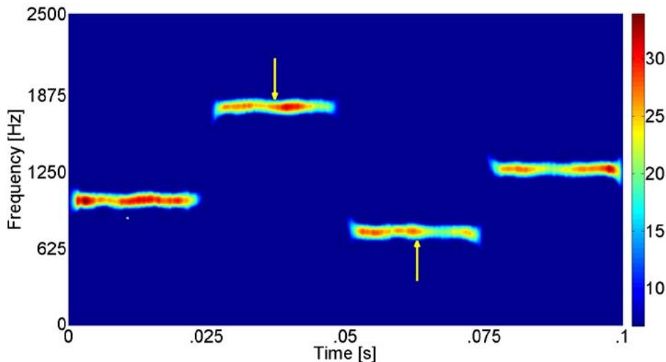 Figure 3: Modulation bandwidth determination for a 4-component frequency hopping signal (512 samples, $\mathrm{SNR} = 10\mathrm{dB}$ ) with threshold value automatically set to $20\%$. From this threshold plot, the modulation bandwidth was measured manually from the highest frequency value of the signal (top yellow arrow) to the lowest frequency value of the signal (bottom yellow arrow) in the y-direction (frequency) 5) Modulation Period: From Figure 4 (which is at a threshold of $20\%$ maximum intensity), the modulation period is the manual measurement of the width of each of the 4 frequency hopping signals in the x-direction (time), and then the average of the 4 signals is calculated. 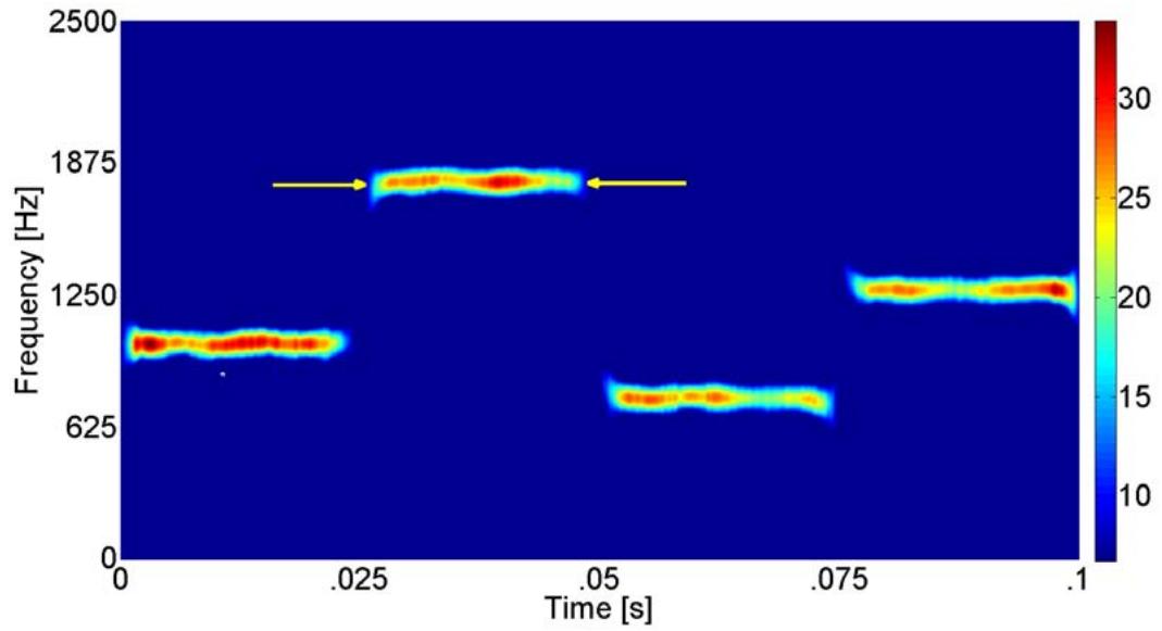 Figure 4: Modulation period determination for a 4-component frequency hopping signal (512 samples, $\mathrm{SNR} = 10\mathrm{dB}$ ) with threshold value automatically set to $20\%$. From this threshold plot, the modulation period was measured manually from the left side of the signal (left yellow arrow) to the right side of the signal (right yellow arrow) in the x-direction (time). This was done for all 4 signal components, and the average value was determined 6) Time-Frequency Localization: From Figure 5, the time-frequency localization is a manual measurement (at a threshold of $20\%$ maximum intensity) of the 'thickness' (in the y-direction) of the center of each of the 4 frequency hopping signal components, and then the average of the 4 values are determined. The average frequency 'thickness' is then converted to: percent of the entire y-axis. 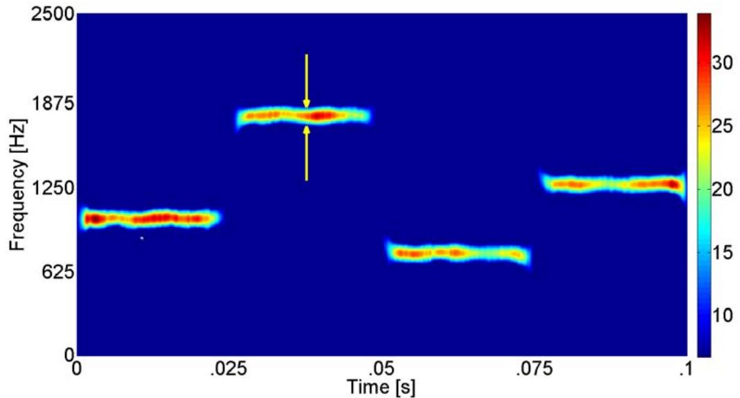 Figure 5: Time-frequency localization determination for a 4-component frequency hopping signal (512 samples, $\mathrm{SNR} = 10\mathrm{dB}$ ) with threshold value automatically set to $20\%$. From this threshold plot, the time-frequency localization was measured manually from the top of the signal (top yellow arrow) to the bottom of the signal (bottom yellow arrow) in the y-direction (frequency). This frequency 'thickness' value was then converted to: $\%$ of entire y-axis 7) Lowest Detectable SNR: The lowest SNR level at which at least a portion of each of the signal components exceeded the set threshold listed in the percent detection section above. For lowest detectable SNR determination, these threshold values (WVD (50%); RSPWVD (50%)) were included in the time-frequency plot algorithms so that the thresholds could be applied automatically during the plotting process. From the threshold plot, the signal was declared a detection if any portion of each of the 4 signal components was visible. The lowest SNR level for which the signal was declared a detection is the lowest detectable SNR. The data from all 100 runs for each test was used to produce the actual, error, and percent error for each of these metrics listed above. The metrics from the WVD were then compared to the metrics from the RSPWVD. By and large, the RSPWVD outperformed the WVD, as will be shown in the results section. ## III. RESULTS Table 1 presents the overall test metrics for the two classical time-frequency analysis techniques used in this testing (WVD versus RSPWVD). Table 1: Overall test metrics (average percent error: carrier frequency, modulation bandwidth, modulation period; average: time-frequency localization-y (as percent of y-axis), percent detection, lowest detectable snr, relative processing time) for the two classical time-frequency analysis techniques (WVD versus RSPWVD) <table><tr><td>Parameters</td><td>WVD</td><td>RSPWVD</td></tr><tr><td>Carrier Frequency</td><td>0.21%</td><td>0.12%</td></tr><tr><td>Modulation Bandwidth</td><td>6.07%</td><td>4.72%</td></tr><tr><td>Modulation Period</td><td>16.51%</td><td>6.05%</td></tr><tr><td>Time-Frequency Localization-Y</td><td>2.14%</td><td>1.28%</td></tr><tr><td>Percent Detection</td><td>90.2%</td><td>94.1%</td></tr><tr><td>Lowest Detectable SNR</td><td>-2.0dB</td><td>-3.0dB</td></tr><tr><td>Relative Processing Time</td><td>0.682s</td><td>0.023s</td></tr></table> From Table 1, the RSPWVD outperformed the WVD in average percent error: carrier frequency (0.12% vs. 0.21%), modulation bandwidth (4.72% vs. 6.07%), modulation period (6.05% vs. 16.51%), and time-frequency localization (y-direction) (1.28% vs. 2.14%); and in average: percent detection (94.1% vs. 90.2%), lowest detectable SNR (-3.0dB vs. -2.0dB) and average relative processing time (0.023s vs. 0.682s). Figure 6 shows comparative plots of the WVD vs. the RSPWVD (4-component frequency hopping) at SNRs of 10dB (top), 0dB (middle), and lowest detectable SNR (-2.0dB for WVD and -3.0dB for RSPWVD) (bottom).       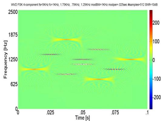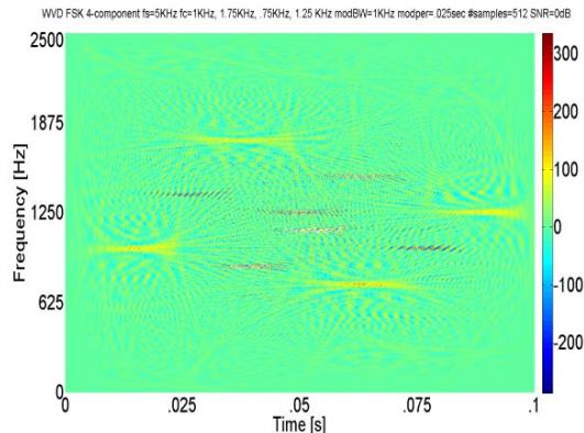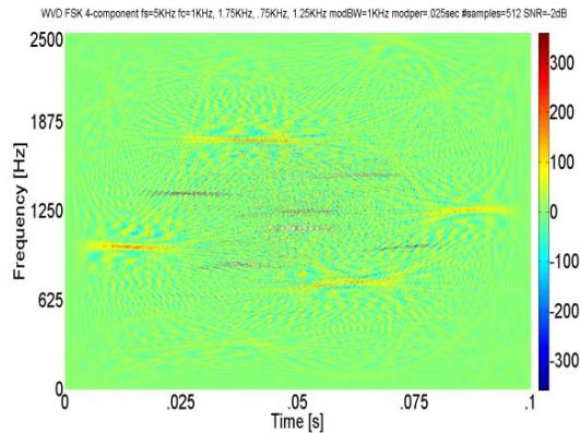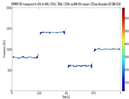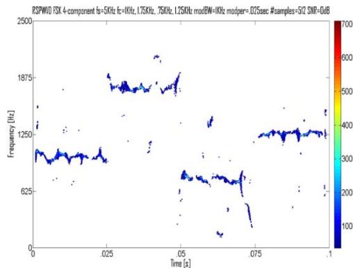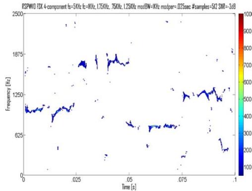Figure 6: Comparative plots for a4-component frequency hopping low probability of intercept radar signals (WVD (left-hand side) vs. RSPWVD (right-hand side)). The SNR for the top row is 10dB, for the middle row is 0dB, and for the bottom row is the lowest detectable SNR(-2dB for WVD and -3dB for RSPWVD). The RSPWVD signals are more localized than the WVD signals. In addition, the WVD does have a cross-term half-way between each signal, which, to the untrained eye, could be misinterpreted as a 'cross-term false positive' (the 6 blue 'false signals') – the more so as the SNR gets lower ## IV. DISCUSSION This section will elaborate on the results from the previous section. relative processing time (0.023s vs. 0.682s). These results are the result of the RSPWVD signal being a more localized signal than the WVD signal, along with the fact that the WVD signal has cross-term interference, which the RSPWVD doesn't have. The RSPWVD might be used in a scenario where you need good signal localization in a fairly low SNR environment, in a short amount of time. The RSPWVD would be preferred over the WVD in virtually every scenario, based on the metrics obtained. ## V. CONCLUSIONS Digital intercept receivers, whose main job is to detect and extract parameters from low probability of intercept radar signals, are currently moving away from Fourier-based analysis and moving towards classical time-frequency analysis techniques, such as the WVD and the RSPWVD, for the purpose of analyzing low probability of intercept radar signals. Based on the research performed for this paper (the novel direct comparison of the WVD versus the RSPWVD for the signal analysis of low probability of intercept frequency hopping radar signals) it was shown that the RSPWVD by and large outperformed the WVD for analyzing these low probability of intercept radar signals - for reasons brought out in the discussion section above. More accurate characterization metrics may well equate to saved equipment and lives. Future plans include analysis of an additional low probability of intercept radar waveform 8-component frequency Hopper, again using the WVD and the RSPWVD as time-frequency analysis techniques. [^1]: Approved for Public Release; Distribution Unlimited: Case Number: AFRL-2022-4315 20220912. _(p.1)_

Generating HTML Viewer...

References

8 Cites in Article
D Adamy (2004). EW 102: A Second Course in Electronic Warfare.
L Anjaneyulu,N Sarma,N Murthy (2009). Identification of LPI radar signals by higher order spectra and neural network techniques.
L Anjaneyulu,N Murthy,N Sarma (2009). Identification of LPI Radar signals by higher order spectra and neural network techniques.
F Auger,P Flandrin,P Goncalves,O Lemoine (1996). Time-Frequency Toolbox Users Manual.
Boualem Boashash,Braham Barkat (2001). Introduction to Time-Frequency Signal Analysis.
R Wiley (2006). ELINT: The Interception and Analysis of Radar Signals.
William Williams,J Jeong (1992). Discrete Reduced Interference Distributions.
Xiang-Gen Xia,V Chen (1999). A quantitative SNR analysis for the pseudo Wigner-Ville distribution.
No ethics committee approval was required for this article type.
Data Availability
Not applicable for this article.
How to Cite This Article
Dr. Daniel L. Stevens. 2026. \u201cA Unique Method for Detecting and Characterizing Low Probability of Intercept Frequency Hopping Radar Signals by means of the Wigner-Ville Distribution and the Reassigned Smoothed Pseudo Wigner-Ville Distribution\u201d. Global Journal of Research in Engineering - F: Electrical & Electronic GJRE-F Volume 22 (GJRE Volume 22 Issue F3).
Explore published articles in an immersive Augmented Reality environment. Our platform converts research papers into interactive 3D books, allowing readers to view and interact with content using AR and VR compatible devices.
Your published article is automatically converted into a realistic 3D book. Flip through pages and read research papers in a more engaging and interactive format.
Our website is actively being updated, and changes may occur frequently. Please clear your browser cache if needed. For feedback or error reporting, please email [email protected]
Thank you for connecting with us. We will respond to you shortly.
Lorem ipsum dolor sit amet, consectetur adipiscing elit. Ut elit tellus, luctus nec ullamcorper mattis, pulvinar dapibus leo.
A Unique Method for Detecting and Characterizing Low Probability of Intercept Frequency Hopping Radar Signals by means of the Wigner-Ville Distribution and the Reassigned Smoothed Pseudo Wigner-Ville Distribution