## I. INTRODUCTION In modern sciences, such as mathematics, physics, astronomy, economics and other sciences, there is little use of differential functions in calculations, because with the help of fractional derivatives and integrals, very few physical, natural, social and other processes are described that use not only the first and second derivatives, single and double integrals, but fractional derivatives and fractional integrals. So in classical mechanics, the first derivative is used as velocity, the second as acceleration, and the third as a jerk. A one-time integral is used to calculate the area under the curve, the mass of an inhomogeneous body, a two-time integral is used to calculate the volume of a cylindrical beam, a three-time integral is used to calculate the volume of the body. They can be found in the equations of mathematical physics, where, in particular, generalized functions and convolutional operations on them are used, and in spectral analysis, and in operational calculus based on integral Fourier and Laplace transformations, and in many other methods where differentiation and integration of functions are used. The basis of all these concepts is the derivative and integral[^1]. Two mathematical operations that are "opposite" to each other, like addition and subtraction, multiplication and division. Two "reciprocal" functions like $\sin(x)$ and $\arcsin(x)$, $x^2$ and $\sqrt{x}$, $e^x$ and $\ln(x)$. Two mathematical operations that logically complement each other, the derivative of the integral does not change the integrable function, as does the integral of the derivative, leaves it unchanged. Let us recall the symbols on graphs and in computer programs. Like any mathematical operation, they have their symbols (designations) on a piece of paper, like ordinary symbols on a computer screen. So, differentiation is denoted as $y'$ or $d/dx$, and integration is $\int y(x) dx$. In this case, a one- time integral is denoted as $\int y(x) dx$, and a two- time integral is $\iint y(x) z(t) dx dt$. With the derivative, the situation is more complicated, it has two designations: $y^\prime$ and $d / dx$. Figure 1 shows (as one of the options) the currently existing designations of differentials and integrals, widely used in the literature.  Figure 1: Notation of integrals and derivatives As can be seen from Figure 1, all the variety of these notations has one property common to all: they try to reflect in various ways, either with the help of numbers or graphically, the order of derivatives or the multiplicity of the integral. In order to unify the record of derivatives and integrals, consider them relative to a certain numerical axis "K" (Figure 2), where the value of the parameter $k$ corresponds to the multiplicity of the integral or the order of the derivative. So, in this scenario of notation, $k = -1$ corresponds to the designation of a single integral $\int y(x) dx$ from the 2nd line and the designation of the same integral $f_{1} * y$ from the 3rd row, and for $k = 1$ - we have the designation of the first derivative $y'$ from the 1st row and the designation of the same first derivative $d / dx$ from the 2nd row. The third line contains the notation of differentials and integrals based on convolutional operations of generalized functions: $y^{(k)} = f_{-k} \star y$, where $k > 0$, a value unequal to an integer is called a fractional derivative of order $k$. An expression of the form: $y_{(k)} = f_{k} \star y$ is called a primitive of order $k$, i.e. an integral of multiplicity $k$ [^1].  Figure 2: Notation of derivatives and integrals for a parabolay(x) = x2 At the same time, all derivatives, including fractional ones, having a negative index, are located on the numerical axis on the right, and all integrals with a positive index - on the contrary, on the left. It was possible to arrange the designations differently, change the plus to minus, but the essence would not change at the same time. There are many types of symbols, binding to the numeric axis requires clarification. To bring these notations in line with the numerical axis$K$, the 4th line contains universal notations for derivatives of any order and integrals of any multiplicity, using angle brackets. The angle brackets denote the order of the derivative or the multiplicity of the integral, for example, $y^{<0>} = y(x)$ is the function under study, and $y^{<1>} = \int y(x) dx$ is its integral, multiplicity 1. So $y^{<2>} = d^2 / dx^2 = y''$ is the second derivative, and $y^{<0,46>}$ is the integral, multiplicity 0,46. For example, a certain derivative of the order of 1,35 is denoted as $y^{<1,35>}$. In other words, if there is a positive number in the angle brackets, it means it is some kind of derivative, and if it is negative, it means it is an integral. And it is easy to read, and it is located correctly on the numeric axis: negative values of the $k$ index are on the left, and positive values are on the right. This form of writing integrals and derivatives is very convenient, for example, for their designation on graphs or diagrams. Figure 2 shows an example of the notation of derivatives and integrals for the parabola $y(x) = x^2$. In addition to notation on graphs, this method can be used for programmers writing programs in various programming languages, for example, {"code_caption":[],"code_content":[{"type":"text","content":"int main() {float y, u, z; int n3; "}],"code_language":"txt"} {"algorithm_caption":[],"algorithm_content":[{"type":"equation_inline","content":"\\begin{array}{l}\\dots \\\\ z = y(4) < 1.5 >;\\\\ u = n3 < - 0,25 >; \\end{array}"}]} where $y^{<1,5>}$ is the derivative of the function $y(4)$ of order 1,5 and $n3^{<0.25>}$ is the integral of multiplicity 0,25 of the function $n3$. In Figure 2, the integral of multiplicity $-0.46$ and the derivative of the order of 1,35 are shown for $x > 0$. It should be borne in mind that when calculating a derivative of a "high" order, say, 123 orders $-y^{<123>}$, previously it was necessary to perform 122 differentiation operations beforehand. This is due to the fact that the definition of the derivative/integral implies an increase in the order of the derivative/integral by only 1. It is impossible, using the existing definition of the derivative, to immediately calculate a high-order derivative from it. Only with the help of sequential multiple calculations can the order of the derivative be increased to the desired value. The same applies to integration. ## II. MATERIALS AND METHODS This method of calculating derivatives reduces the efficiency of using the differentiation operation, for example, in series expansions, because it requires calculating derivatives of a "high" order, and this is time-consuming and involves calculation errors. Therefore, in such calculations, only the first few terms of the decomposition are taken, and the rest are discarded, which increases the calculation error. As for calculating integrals, especially multiplicities greater than 2, this is an even more difficult task. Thus, the lack of a simple, reliable and accurate method of differentiation and/or integration significantly hinders computational progress in mathematics. The same problem is observed in physics. Many laws of mathematical physics, most often appearing in simple, accessible calculations, are based on the use, mainly, of the 1st, maximum 2nd derivative (for example, current $i = dq / dt$, force $F = m \cdot d^2 x / dt^2$ ) and a single integral, for example, voltage across the capacitor $u(t) = 1 / C \cdot \int i(t)dt$. It is very rare in everyday physics or mathematics to find a 3rd derivative or a 3-fold integral. This does not happen often. One of the ways to use a 3-fold integral is the Ostrogradsky-Gauss integral to calculate the volume of a body if the surface bounding this body is known. And if you look more broadly, then neither in physics nor in mathematics have the everyday laws of the universe using fractional derivatives and integrals been discovered so far, because their calculation is fraught with great difficulties [^1]. At the same time, it is possible that all the diversity of the world exists exactly there, in a fractional dimension, which can be described and studied, precisely with the help of fractional (analog), and not integer (discrete) integrals and differentials. Take, for example, the mechanism of describing multidimensional structures, for example, multidimensional space. Our 3-dimensional space and one-dimensional time are described by discrete (integer) coordinate values, in this case one and three. At the same time, the question of the existence of a space having, not 3, but, say, 2,345 coordinates is of great scientific and practical interest. In other words, the structure of a special "fractional" space, no longer two-dimensional, is a plane (because to describe the plane, you need 2 coordinates, and we have more - 2,345), but also not a three-dimensional volume (where 3 coordinates are needed), i.e. something average between the plane and the volume. It is very difficult to imagine such a structure. In nature, such a space does not seem to exist. It is even more difficult to determine the velocity or acceleration in such a space, i.e. to describe the kinematics of the motion of bodies. If it is possible to define the force in such a space (or to use the already existing classical method of specifying forces), then we can count on success in creating the dynamics of such structures, i.e., in other words, to create the mechanics of multidimensional space. At the same time, our classical 3-dimensional mechanics will turn out to be a special case of a more general mechanics - the mechanics of multidimensional spaces. This can be said about other physical laws of the universe. And whether our idea of the world will change with the emergence of a new, more general, idea of space. So far we don't know much about this, because our concepts are tied to a three-dimensional dimensional space, and all the diversity of the world "lies" in a multidimensional "fractional" world that has not been studied at all. A number of legitimate questions arise: - What kind of space is "located", say, between a plane (2-dimensional space) and a volume (3-dimensional), i.e. a substance with the dimension of space $R$, where $2 < R < 3$? - What kind of physical quantity, which is between speed and acceleration between $y^{<1>}$ and $y^{<2>}$ from the move, i.e. a physical quantity, defined, for example, the fractional derivative of $y^{<1,23>}$, the order of 1,23 (not 1 or 2)? - Whether Newton's laws are applicable to the so-called fractional space? - How will the definition of force in fractional space change (if it changes)? - Will it be possible to apply the classical laws of mechanics to fractional space, or will it be necessary to create a new, more general, mechanics of the macro and microcosm? - Will the interaction between space and time change if we "replace" the classical concept of space with a fractional one? - Will there be changes in Einstein's theory of relativity and will the concepts of "gravitational, electromagnetic and other interactions" and much, much more remain the same? Answers to these and other questions can be obtained if you have a convenient apparatus for calculating derivatives/integrals of any order/multiplicity, including fractional ones. In other words, it is necessary to create such a calculation algorithm, simple and convenient, especially for novice researchers, where instead of calculating integrals/differentials, it would be possible to use the usual substitution of numbers, in which the desired order or multiplicity could be set without performing calculations, but simply substitute the desired parameter into the desired formula and get a ready derivative/integral without their calculations, i.e. immediately. Such a tool, which could be called, for example, functions - $SL(x,k)$, would greatly simplify the process of calculating derivatives and integrals and significantly expand the boundaries of our knowledge. First, we introduce the concepts of a differential integral function based on the definition of a differential integral. The differential integral function $SL(x,k)$ is an ordinary function of several arguments, where, separated by commas, its arguments (in this case one - $x$ ) and the parameter $k$, the order of future derivatives and/or the multiplicity of integrals are indicated[^2]. For example, for a parabola $y(x) = x^2$, such a differential integral function $SL(x,k)$ will have the form[^3]. $$ S L (x, k) := 2 \cdot \frac {x ^ {2 - k}}{\Gamma (3 - k)} \tag {1} $$ where, $x$ is the argument of the function, $k$ is a parameter that specifies the order of the derivative or the multiplicity of the integral. This is the differential integral function of a parabola, the usual function of 2 arguments, argument $x$ and parameter $k$. It represents a whole set of integrals and derivatives of any order and multiplicity[^4](the main, mother function). How to use it? You need to set the parameter $k$ and get the desired derivative or integral. For example, for a parabola, we substitute $k = 0$ into it. Then, for $k = 0y(x,k) = x^2$, $(\Gamma (3 - k) = 2)^5$ the function (parabola) does not change. When $k = 1y(x,k) = 2x$ and the parabola is transformed into its 1st derivative $y^{<1>}$. When $k = -1y(x,k) = x^3 / 3$ and the function becomes its one-time integral $-y^{<-1>}$, and for $k = -2y(x,k) = x^4 / 12$ double $-y^{<-2>}$. No calculations, just substitution. Fractional derivatives and integrals are of particular interest, because there is no simple and reliable way to calculate them, except for the method indicated above [^2]. In this case, the method of obtaining is the same. To calculate them, it is enough to substitute the necessary value of the derivative instead of the parameter $k$, for example, $k = 0.123$ and the parabola becomes its derivative of the order $0.123 - y < 0.123 >$: $$ S L (x, k) := 2 \cdot \frac {x ^ {2 - 0 , 1 2 3}}{\Gamma (3 - 0 , 1 2 3)} f l o a t, 3 \rightarrow 1, 1 2 \tag {2} $$ If it is necessary to obtain an integral of multiplicity $3,45 - y^{<-3,45>}$, it is enough to substitute $k = -3,45$ into the differential function (1) and the parabola becomes its integral of multiplicity $3,45 - y^{<-3,45>}$: $$ S L (x, k) := 2 \cdot \frac {x ^ {2 + 3 , 4 5}}{\Gamma (3 + 3 , 4 5)} f l o a t, 3 \rightarrow 7, 6 0 6 0 ^ {- 3} x ^ {5, 4} \tag {3} $$ This method of calculating fractional derivatives is no different from the method of obtaining integer (discrete) derivatives - the same substitution. There is no difference between an integer or fractional derivative/integral. Simple substitution to get a given result. Consider another example: $y(x) = \sin (x)$. For a sine wave, the differential integral function $SL(x,k)$ will have the following form: $$ S L (x, k) := \sin \left(x + k \cdot \frac {\pi}{2}\right) \tag {4} $$ This is a sine wave whose phase shift depends on the order of its derivative/multiplicity of its integral. At $k = 0$, the sine wave does not change, at $k = 1$, and becomes $\cos(x)$, i.e., its first derivative is $y^{<1>}$, and at $k = -1$ it becomes $-\cos(x)$, i.e., its integral is $y^{<1>}$. At $-1 < k < 1$, the function occupies an intermediate position between $-\cos(x)$ and $\cos(x)$, including $\sin(x)$ at $k = 0$. The differential integral function for the sine wave (4) is a graphical representation of the differential integral function, namely, the parameter $k$ represents a part of the right angle for unit orts. At $k = 1$, the function $SL(x,1)$ becomes the 1st derivative, such a unit ort is perpendicular to the abscissa axis, and at $k = \text{var}$ it is a fractional derivative of $k$ order and the angle $k$ (in values from 0 to 1 or in% of 90 degrees) it is only a part of the right angle. For the exponent $y(x) = e^{x}$, the differential integral function $SL(x, k)$ does not depend on $k$ and all its derivatives and integrals are equal to each other and equal to the exponent itself. These examples can be summarized in Table 1, where its derivatives and integrals are given for some elementary functions. Table 1: Examples of calculation of derivatives and integrals <table><tr><td>y&lt;sup&lt;-1&gt;</td><td>y&lt;sup&lt;-0.5&gt;</td><td>y&lt;sup&gt;0&gt;</td><td>y&lt;sup&gt;0.5&gt;</td><td>y&lt;sup&gt;1.5&gt;</td><td>SL (x, k)</td></tr><tr><td>Γ (n+1)xn+1/Γ (n+2)</td><td>Γ (n+1)xn+0.5/Γ (n+1,5)</td><td>xn</td><td>Γ (n+1)xn-0.5/Γ (n+0,5)</td><td>Γ (n+1)xn-1.5/Γ (n-0,5)</td><td>Γ (n+1)xn-k/Γ (n+1-k)</td></tr><tr><td>x3/3</td><td>0,601x2.5</td><td>x2</td><td>1,504x1.5</td><td>2,256x0.5</td><td>2 x2-k/Γ (3-k)</td></tr><tr><td>ex</td><td>ex</td><td>ex</td><td>ex</td><td>ex</td><td>ex</td></tr><tr><td>sin(x-π/2)</td><td>sin(x-0,5:π/2)</td><td>sin(x)</td><td>sin(x+0,5:π/2)</td><td>sin(x+1,5:π/2)</td><td>sin (x+k:π/2)</td></tr></table> Differential functions can be a function of 2 or more arguments, for example, $SL(x,y,k)$, where $(x)$ and $(y)$ are two arguments of the same function: $SL(x,y,k_x,k_y) = 2\cdot k_y + (x - y)\cdot k_x$, and $k_{x}$ and $k_{y}$ are still a parameter. In addition, any continuous elementary function can be used as a parameter, including the same differential integral function, for example: $$ (x,y,k1,k2) := x^{\sin\left(y\cdot k1+\frac{\pi}{2}k2\right)} $$ Of particular interest is the differential integral function, in which the parameter $k$ is a complex number $s$, $s = a + i \cdot b$, although in general, the parameter $k$ can be any function of a real or complex argument. ## III. RESEARCH RESULTS To obtain the differential integral function, we recall the Laplace integral transformation and Borel's theorem. The integral Laplace transform has the form $$ L[f(t)] = F(s) = \int_0^\infty f(t)e^{-st} dt \equiv [f(t)\cdot e^{-st} dt]^{<-1>_{0<t<\infty}} $$ where $s = a + i^* b$ is a complex quantity. Here $f(t)$ is the original function, and $F(s)$ is its Laplace image. This is a direct conversion of the original into an image. The inverse Laplace transform $$ f (t) := \frac {1}{2 \pi i} \cdot \int_ {\sigma - i \cdot \infty} ^ {\sigma + i \cdot \infty} e ^ {s t} F (s) d s \equiv \left[ e ^ {s t} \cdot F (s) \cdot d s \right] ^ {< - 1 > _ {\sigma - i \infty < \sigma + i \infty}} \tag {7} $$ it is necessary to find the original of the function by its image. Let's consider one of the main properties of this transformation – the differentiation of the original function. Let $L[f(t)] = F(s)$. Let's find $L[f(t)^{<1>}$, where $f(t)^{<1>}$ is the 1st derivative, and $L[f(t)^{<1>}]$ its image. $$ L[f(t)^{<1>}] = [f(t)^{<1>}\cdot e^{-st}dt]^{<-1>_{0<t<\infty}} = e^{-st}\cdot f(t)_{0<t<\infty} + s\cdot [f(t)\cdot e^{st}dt]^{<-1>_{0<t<\infty}} $$ If for $t \to \infty$ the function $f(t)$ increases no faster than $M^* e^{at}$, then $\mathrm{e}^{-st}\star f(t)\rightarrow 0$ for $t\to \infty$ and is equal to $f(0)$,and $$ L [ f (t) ^ {< 1 >} ] = s ^ {*} F (s) - f (0) \tag {9} $$ For $f(0) = 0$ $$ L [ f (t) ^ {< 1 >} ] = s * F (s) \tag {10} $$ and the differentiation of the original function corresponds to the multiplication of the image of the function by $s$. Let's consider another important property – the integration of the original. If $g(t) = [f(\tau)d\tau]^{<t>}$ then under zero initial conditions $g(t)^{<t>} = f(t)$ and $$ L[g(t)^{<1>}] = L[f(t)] = s * L[g(t)] = s * L[\int_0^t f(\tau) d\tau]^{<-1>} $$ Since $L[f(t)] = F(s)$, then $$ L \left[ \left[ f (\tau) ^ {*} d \tau \right] _ {0 < \tau < t} ^ {- t >} = F (s) / s \right. \tag {12} $$ that is, the integration of the function corresponds to the division of the image $F(s)$ by $s$. Taking into account expressions (14) and (16), we can conclude that the operations of differentiation/integration of the original can be replaced by algebraic actions (multiplication/division by $s$ ) on their images [^3]. Thanks to this replacement, this method has found the widest application in integral and differential calculus [4]. However, the case is of particular interest when the function is represented as $$ L [ f (t) ] = F (s) / \left( s ^ { - k } \right) $$ that is, the image is divided by $(s - k)$. In this case, depending on $k$, we get fractional derivatives/integrals. For $k > 0$, fractional derivatives of the order $k$ are formed, and for $k < 0$, fractional integrals of the same multiplicity are formed. $$ L [ f (t) ] = \frac{\mathrm{F} (s)}{s ^ {- k}} = 1 / (\Gamma (- k)) $$ $$ SL\left(x,k\right) = L\left[f\left(t\right)\right] $$ These expressions (18) and (19) define fractional derivatives/integrals of order $k$, and are the differential functions of the desired function $f(t)$. Examples of these functions are shown in Table 1. Let's consider some examples of the use of differential integral functions in solving approximation problems. Suppose must be approximated by a power series $p \overline{a} \cos(x)$ in a neighborhood of the point $x0$, the function $\cos(x)$, and choose the polynomial coefficients $a_0 \ldots a_5$ so as to minimize the mean square error of approximation of this polynomial are: $$ _\cos(x) = a_0 + a_1 x + a_2 x^2 + a_3 x^3 + a_4 x^4 + a_5 x^5 $$ and at the selected point is known for its derivatives and differentials, as an integer and the fraction. To do this, we fulfill the approximation conditions according to which the value of the polynomial $\cos(x)$ and its fractional derivatives (for simplicity of calculation, only six (5) derivatives are used[^6]. To increase the accuracy, you can use more, for example, several dozen derivatives, the computer allows it. Instead of derivatives, its integrals can also be used in the same way) in the vicinity of a given point $x_0$, from the domain of the polynomial definition, should equal the corresponding values of the desired function $\cos(x)$ and its fractional derivatives (and integrals). 2 points are selected as points $-x = 3$ and $x = 15$. The fractional derivatives/integrals for the elements of the polynomial are defined as $$ S L (x, n, k) := \frac {\Gamma (n + 1) \cdot x ^ {n - k}}{\Gamma (n + 1 - k)} \tag {17} $$ where $x$ -is the matrix of diagnostic information; $n$ - is the exponent of the polynomial; $k$ - is a parameter that sets the multiplicity of the integral or the order of derivatives. Further, solving a linear algebraic equation of the form: $$ a = A 1 ^ {- 1} \cdot B 1 \tag {18} $$ we obtain the solution of this equation in the form of the desired coefficients $a_0\ldots a_5$ (Application A Figure A.1). The solution was made in the MathCad program, the calculation listing is given for the point $x = 3$ and additionally for $x = 15$. Another example. In addition to the approximation at a point, using the differential integral functions, it is possible to approximate on a given segment. Examples of this approximation are given below. Let it be necessary to approximate, for simplicity, the known functions $\cos (x)$ and the exponent $\exp (x)$, as well as $\cos (x)$ on the plot $4 < x < 6$, as well as volume curves, according to the type of Fleicher-Manson or Robinson-Dadson curves. For ease of calculation, we approximate 6 points for 2 cos $(x)$ functions, 4 (four) points for the exponent $\exp (x)$ and 23 for volume curves. For a sine wave, the desired points will be of two types. In the first case, these are the points -5, -4, -2, 1, 3, 5. In the second case, this is -5, -3, -1, 1, 3, 5. We will approximate the sinusoid with a polynomial (17). Exponent - exponent. For the first case, for points -5, -4, -2, 1, 3, 5 the initial data obtained by formula (17) will have the following form. $$ \mathrm {A} 2 := \left( \begin{array}{r r r r r r} 1 & - 5 & 2 5 & - 1 2 5 & 6 2 5 & - 3 1 2 5 \\1 & - 4 & 1 6 & - 6 4 & 2 5 6 & - 1 0 2 4 \\1 & - 2 & 4 & - 8 & 1 6 & - 3 2 \\1 & 1 & 1 & 1 & 1 & 1 \\1 & 3 & 9 & 2 7 & 8 1 & 2 4 3 \\1 & 5 & 2 5 & 1 2 5 & 6 2 5 & 3 1 2 5 \end{array} \right) \qquad \mathrm {B} 2 := \left( \begin{array}{l} \cos (- 5) \\\cos (- 4) \\\cos (- 2) \\\cos (1) \\\cos (3) \\\cos (5) \end{array} \right) \qquad \mathrm {b} 2 := \mathrm {A} 2 ^ {-} \mathbf {\Phi} ^ {-} \cdot \mathrm {B} 2 \quad \mathrm {b} 2 = \left( \begin{array}{l} 0. 6 1 5 \\0. 2 0 7 \\- 0. 2 5 7 \\- 0. 0 3 6 \\9. 7 3 1 \times 1 0 ^ {- 3} \\1. 1 1 7 \times 1 0 ^ {- 3} \end{array} \right) $$ As a result of calculating the series $rjad\_cos(x)$, we get the values of $\cos(x)$. $$ rjad_1_cos(x) := b2_0 + b2_1 + b2_2 \cdot x^2 + b2_3 \cdot x^3 + b2_4 \cdot x^4 + b2_5 \cdot x^5 $$ The graphs of these two functions $\cos(x)$ and $rjad_1\cos(x)$ and some values of these graphs are shown in Figure 3. 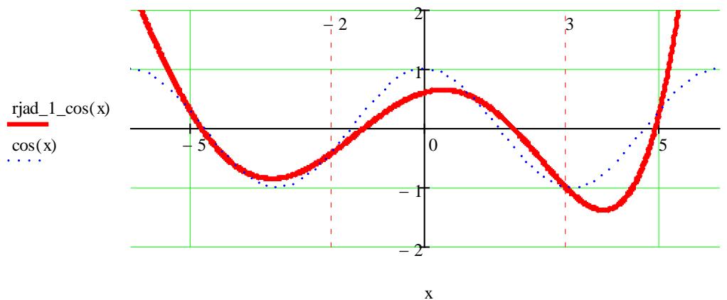 Figure 3: Values of the functions $rjad_1\cos (x)$ and $\cos (x)$ $$ r j a d _ {1} \text{cos} (- 5) = 0.2 8 4 $$ $$ \cos (- 5) = 0. 2 8 4 $$ $$ rjad_1_cos(-2) = -0.416 $$ $$ \cos (- 2) = - 0. 4 1 6 $$ $$ rjad_1_cos(3) = -0.99 $$ $$ \cos (3) = - 0. 9 9 $$ $$ rjad_1_cos(-4) = -0.654 $$ $$ \cos(-4) = -0.284 $$ $$ rjad_1_cos(-1) = 0.54 $$ $$ \cos (- 1) = 0. 5 4 $$ $$ r j a d _ {1} \text{cos} (5) = 0.2 8 4 $$ $$ \cos (5) = 0. 2 8 4 $$ For another cosine, for the values -5, -3, -1, 1, 3, 5 the initial data obtained by the formula (17) will have the following form: $$ \mathrm {A 3} := \left( \begin{array}{l l l l l l} \mathrm {S L} \bigl (- x _ {0}, - n _ {0}, 0 \bigr) & \mathrm {S L} \bigl (- x _ {0}, - n _ {1}, 0 \bigr) & \mathrm {S L} \bigl (- x _ {0}, - n _ {2}, 0 \bigr) & \mathrm {S L} \bigl (- x _ {0}, - n _ {3}, 0 \bigr) & \mathrm {S L} \bigl (- x _ {0}, - n _ {4}, 0 \bigr) & \mathrm {S L} \bigl (- x _ {0}, - n _ {5}, 0 \bigr) \\\mathrm {S L} \bigl (- x _ {1}, - n _ {0}, 0 \bigr) & \mathrm {S L} \bigl (- x _ {1}, - n _ {1}, 0 \bigr) & \mathrm {S L} \bigl (- x _ {1}, - n _ {2}, 0 \bigr) & \mathrm {S L} \bigl (- x _ {1}, - n _ {3}, 0 \bigr) & \mathrm {S L} \bigl (- x _ {1}, - n _ {4}, 0 \bigr) & \mathrm {S L} \bigl (- x _ {1}, - n _ {5}, 0 \bigr) \\\mathrm {S L} \bigl (- x _ {2}, - n _ {0}, 0 \bigr) & \mathrm {S L} \bigl (- x _ {2}, - n _ {1}, 0 \bigr) & \mathrm {S L} \bigl (- x _ {2}, - n _ {2}, 0 \bigr) & \mathrm {S L} \bigl (- x _ {2}, - n _ {3}, 0 \bigr) & \mathrm {S L} \bigl (- x _ {2}, - n _ {4}, 0 \bigr) & \mathrm {S L} \bigl (- x _ {2}, - n _ {5}, 0 \bigr) \\\mathrm {S L} \bigl (- x _ {3}, - n _ {0}, 0 \bigr) & \mathrm {S L} \bigl (- x _ {3}, - n _ {1}, 0 \bigr) & \mathrm {S L} \bigl (- x _ {3}, - n _ {2}, 0 \bigr) & \mathrm {S L} \bigl (- x _ {3}, - n _ {3}, 0 \bigr) & \mathrm {S L} \bigl (- x _ {3}, - n _ {4}, 0 \bigr) & \mathrm {S L} \bigl (- x _ {3}, - n _ {5}, 0 \bigr) \\\mathrm {S L} \bigl (- x _ {4}, - n _ {0}, 0 \bigr) & \mathrm {S L} \bigl (- x _ {4}, - n _ {1}, 0 \bigr) & \mathrm {S L} \bigl (- x _ {4}, - n _ {2}, 0 \bigr) & \mathrm {S L} \bigl (- x _ {4}, - n _ {3}, 0 \bigr) & \mathrm {S L} \bigl (- x _ {4}, - n _ {4}, 0 \bigr) & \mathrm {S L} \bigl (- x _ {4}, - n _ {5}, 0 \bigr) \\\mathrm {S L} \bigl (- x _ {5}, - n _ {0}, 0 \bigr) & \mathrm {S L} \bigl (- x _ {5}, - n _ {1}, 0 \bigr) & \mathrm {S L} \bigl (- x _ {5}, - n _ {2}, 0 \bigr) & \mathrm {S L} \bigl (- x _ {5}, - n _ {3}, 0 \bigr) & \mathrm {S L} \bigl (- x _ {5}, - n _ {4}, 0 \bigr) & \mathrm {S L} \bigl (- x _ {5}, - n _ {5}, 0 \bigr) \end{array} \right) $$ $$ \mathrm{B}3 := \left( \begin{array}{l} \cos (- 5) \\\cos (- 3) \\\cos (- 1) \\\cos (1) \\\cos (3) \\\cos (5) \end{array} \right) \quad - x := \left( \begin{array}{l} - 5 \\- 3 \\- 1 \\1 \\3 \\5 \end{array} \right) \quad d = A3^{-1} B3 $$ $$ rjad_2_cos(x) := d_0 + d_1 x + d_2 x^2 + d_3 x^3 + d_4 x^4 + d_5 x^5 $$ The graphs of these two functions $\cos(x)$ and $rjad_2\cos(x)$ and some values of these graphs are shown in Figure 4. 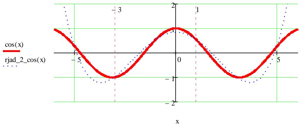 Figure 4: Values of the functions - rjad_2_cos (x) and cos (x) $$ \begin{array}{c} r j a d \_ 2 \_ c o s (- 5) = 0. 2 8 4 \\\cos (- 5) = 0. 2 8 4 \end{array} $$ $$ rjad_2_cos(1) = 0.54\cos(1) = 0.54 $$ $$ \begin{array}{c} r j a d \_ 2 \_ c o s (- 3) = - 0. 9 9 \\\cos (- 3) = - 0. 9 9 \end{array} $$ $$ rjad_2_cos(-3) = -0.99\cos(3) = -0.99 $$ $$ \begin{array}{c} r j a d \_ 2 \_ c o s (- 1) = 0. 5 4 \\\cos (- 1) = 0. 5 4 \end{array} $$ $$ rjad_2_cos(5) = 0.284\cos(5) = 0.284 $$ If we look at the same graphs in other coordinates, we can say that at these points the graphs coincide with their values, and at other points they do not, and they differ significantly. 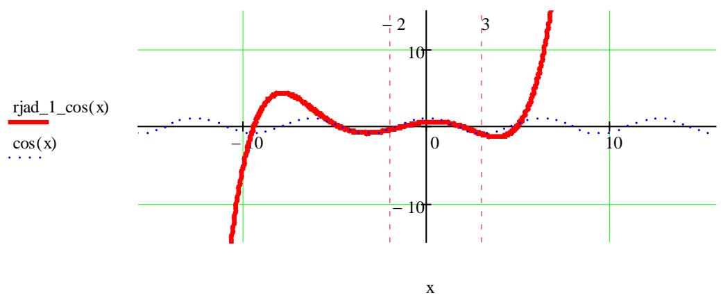 Figure 5: Values of the functions $rjad\_1\_cos(x)$ and $\cos(x)$ The values of these two functions $r \text{rad}_1 \cos(x)$ and $\cos(x)$ in other coordinate systems coincide only in this section in $\pm 2\pi$, and for other values of the argument they differ greatly. Figure 6 shows the values of these two functions $rjad\_2\_cos(x)$ and $\cos (x)$. In the given figure shows that the values of these two functions $rjad\_2\_cos(x)$ and $\cos (x)$ in different coordinate systems coincide only in this region of $\pm 6$, and for other values of the argument vary greatly. This suggests that approximation by differential integral functions is possible both at a point and at a certain area. The approximation error is minimal and can be reduced by increasing the number of terms of the polynomial. 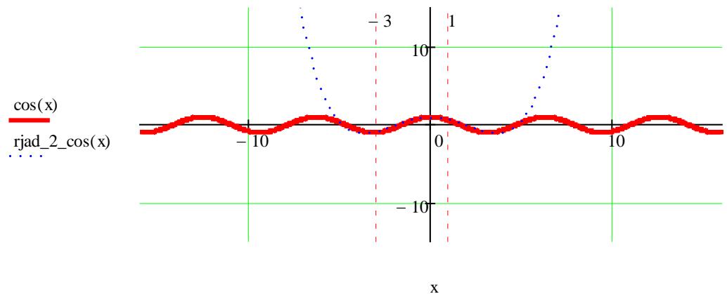 Figure 6: Values of the functions $\text{rjad\_2\_cos}(\mathbf{x})$ and $\cos(\mathbf{x})$ The exponent can be approximated by the exponent itself. An example is shown below in Figure 7. $$ \begin{array}{c c c c c} \text {n} & 0 & 1 & 2 & 3 \end{array} $$ $$ \mathrm{A}1 := \left( \begin{array}{c c c c} 1^{0} & 1^{1} & 1^{2} & 1^{3} \\2^{0} & 2^{1} & 2^{2} & 2^{3} \\7^{0} & 7^{1} & 7^{2} & 7^{3} \\10^{0} & 10^{1} & 10^{2} & 10^{3} \end{array} \right) $$ $$ \mathrm{B}1 := \left( \begin{array}{l} \mathrm{e}^{1} \\\mathrm{e}^{2} \\\mathrm{e}^{7} \\\mathrm{e}^{10} \end{array} \right) \quad \quad \quad \mathrm{a} := \mathrm{A}1^{-1} \cdot \mathrm{B}1 \quad \quad \mathrm{a} = \left( \begin{array}{l} -1.19 \times 10^{3} \\1.966 \times 10^{3} \\-863.71 \\89.924 \end{array} \right) $$ $$ \mathrm{k} := (1 2 7 1 0)^{\mathrm{T}} $$ $$ e ^ {k} = \left( \begin{array}{c} 2. 7 1 8 \\7. 3 8 9 \\1. 0 9 7 \times 1 0 ^ {3} \\2. 2 0 3 \times 1 0 ^ {4} \end{array} \right) $$ $$ r j a d _ {-} \exp (x) := a _ {0} + a _ {1} x + a _ {2} x ^ {2} + a _ {3} x ^ {3} \tag {21} $$ $$ rjad_exp(1) = 2.718\quad e^{1} = 2.718 $$ $$ rjad_exp(2) = 7.389\quad e^{2} = 7.389 $$ $$ rjad_exp(7) = 1.097 \times 10^{3} $$ $$ rjad_exp(10) = 2.203 \times 10^{4} $$ Figure 7 shows the values of these two functions - $r\text{jad\_exp}(x)$ and $\exp(x)$. 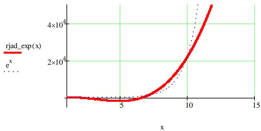 Figure 7: Values of the functions - rjad_exp (x) and exp (x) The graph of the $\cos(x)$ function on the section from $x = 4$ to $x = 6$ and the initial data are shown below in Figure 8. $$ k_{-1} := 1 + 1 \cdot 10^{-6} $$ $$ \operatorname {S L} (\mathrm {x}, \mathrm {k}, \mathrm {n}) := \frac {\mathrm {x} ^ {\mathrm {n} - \mathrm {k}} \cdot \Gamma (\mathrm {n} + 1)}{\Gamma (\mathrm {n} - \mathrm {k} + 1)} $$ The set point - $\mu$ $$ \mu := 5 $$ $$ A1 := \left( \begin{array}{c c c c c c} 1 & \mu & \mu^ {2} & \mu^ {3} & \mu^ {4} & \mu^ {5} \\\frac{\mu^ {- 0 . 2 5} \cdot \Gamma (1)}{\Gamma (1 - 0 . 2 5)} & \frac{\mu^ {1 - 0 . 2 5}}{\Gamma (2 - 0 . 2 5)} & \frac{2 \cdot \mu^ {2 - 0 . 2 5}}{\Gamma (3 - 0 . 2 5)} & \frac{6 \cdot \mu^ {3 - 0 . 2 5}}{\Gamma (4 - 0 . 2 5)} & \frac{2 4 \cdot \mu^ {4 - 0 . 2 5}}{\Gamma (5 - 0 . 2 5)} & \frac{1 2 0 \cdot \mu^ {5 - 0 . 2 5}}{\Gamma (6 - 0 . 2 5)} \\\frac{\mu^ {- 0 . 5} \cdot \Gamma (1)}{\Gamma (1 - 0 . 5)} & \frac{\mu^ {1 - 0 . 5}}{\Gamma (2 - 0 . 5)} & \frac{2 \cdot \mu^ {2 - 0 . 5}}{\Gamma (3 - 0 . 5)} & \frac{6 \cdot \mu^ {3 - 0 . 5}}{\Gamma (4 - 0 . 5)} & \frac{2 4 \cdot \mu^ {4 - 0 . 5}}{\Gamma (5 - 0 . 5)} & \frac{1 2 0 \cdot \mu^ {5 - 0 . 5}}{\Gamma (6 - 0 . 5)} \\\frac{\mu^ {- 0 . 7 5} \cdot \Gamma (1)}{\Gamma (1 - 0 . 7 5)} & \frac{\mu^ {1 - 0 . 7 5}}{\Gamma (2 - 0 . 7 5)} & \frac{2 \cdot \mu^ {2 - 0 . 7 5}}{\Gamma (3 - 0 . 7 5)} & \frac{6 \cdot \mu^ {3 - 0 . 7 5}}{\Gamma (4 - 0 . 7 5)} & \frac{2 4 \cdot \mu^ {4 - 0 . 7 5}}{\Gamma (5 - 0 . 7 5)} & \frac{1 2 0 \cdot \mu^ {5 - 0 . 7 5}}{\Gamma (6 - 0 . 7 5)} \\\frac{\mu^ {- k _ {-} 1} \cdot \Gamma (1)}{\Gamma (1 - k _ {-} 1)} & \frac{\mu^ {1 - 1}}{\Gamma (2 - 1)} & \frac{2 \cdot \mu^ {2 - 1}}{\Gamma (3 - 1)} & \frac{6 \cdot \mu^ {3 - 1}}{\Gamma (4 - 1)} & \frac{2 4 \cdot \mu^ {4 - 1}}{\Gamma (5 - 1)} & \frac{1 2 0 \cdot \mu^ {5 - 1}}{\Gamma (6 - 1)} \\\frac{\mu^ {- 1 . 2 5} \cdot \Gamma (1)}{\Gamma (1 - 1 . 2 5)} & \frac{\mu^ {1 - 1 . 2 5}}{\Gamma (2 - 1 . 2 5)} & \frac{2 \cdot \mu^ {2 - 1 . 2 5}}{\Gamma (3 - 1 . 2 5)} & \frac{6 \cdot \mu^ {3 - 1 . 2 5}}{\Gamma (4 - 1 . 2 5)} & \frac{2 4 \cdot \mu^ {4 - 1 . 2 5}}{\Gamma (5 - 1 . 2 5)} & \frac{1 2 0 \cdot \mu^ {5 - 1 . 2 5}}{\Gamma (6 - 1 . 2 5)} \end{array} \right) $$ $$ \mathrm{B}1 := \left( \begin{array}{l} \cos \left(\mu + 0.00\cdot\frac{\pi}{2}\right) \\\cos \left(\mu + 0.25\cdot\frac{\pi}{2}\right) \\\cos \left(\mu + 0.50\cdot\frac{\pi}{2}\right) \\\cos \left(\mu + 0.75\cdot\frac{\pi}{2}\right) \\\cos \left(\mu + 1.00\cdot\frac{\pi}{2}\right) \\\cos \left(\mu + 1.25\cdot\frac{\pi}{2}\right) \end{array} \right) $$ $$ \mathbf{a} = \mathrm{A1}^{-1} \mathrm{B1} $$ $$ -\cos (x) := a_{0} + a_{1}\cdot x + a_{2}\cdot x^{2} + a_{3}\cdot x^{3} + a_{ 4}\cdot x^{4} + a_{5}\cdot x^{5} $$ $$ \cos (5) = 2,836622\cdot 10^{-1} $$ $$ \cos (5) = 2, 8 3 6 6 2 2 \cdot 1 0 ^ {- 1} $$  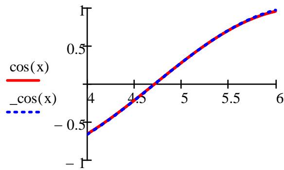X Figure 8: Values of the functions - $\cos (x)$ and $-\cos (x)$ Additionally, the application of differential integration functions in music, curves of equal loudness, for example, Fletcher-Manson curves or Robinson-Dudson curves, Figure 9, is presented. <table><tr><td rowspan="4">KRG=</td><td>0</td><td>1</td><td>2</td><td>3</td><td>4</td><td>5</td><td>6</td><td>7</td><td>8</td><td>9</td><td>10</td><td>11</td><td>12</td><td>13</td><td>14</td><td>15</td><td>16</td><td>17</td><td>18</td><td>19</td><td>20</td><td>21</td><td>22</td><td>23</td><td></td></tr><tr><td>0</td><td>20</td><td>40</td><td>63</td><td>100</td><td>160</td><td>200</td><td>250</td><td>315</td><td>400</td><td>500</td><td>630</td><td>800</td><td>1·103</td><td>1.25·103</td><td>1.6·103</td><td>2·103</td><td>2.5·103</td><td>3.15·103</td><td>4·103</td><td>5·103</td><td>6.3·103</td><td>8·103</td><td>1·104</td><td>1.25·10</td></tr><tr><td>1</td><td>2.996</td><td>3.689</td><td>4.143</td><td>4.605</td><td>5.075</td><td>5.298</td><td>5.521</td><td>5.753</td><td>5.991</td><td>6.215</td><td>6.446</td><td>6.685</td><td>6.908</td><td>7.131</td><td>7.378</td><td>7.601</td><td>7.824</td><td>8.055</td><td>8.294</td><td>8.517</td><td>8.748</td><td>8.987</td><td>9.21</td><td>9.43</td></tr><tr><td>2</td><td>119</td><td>105.3</td><td>98.4</td><td>92.5</td><td>87.8</td><td>85.9</td><td>84.3</td><td>82.9</td><td>81.7</td><td>80.9</td><td>80.2</td><td>79.7</td><td>80</td><td>82.5</td><td>83.7</td><td>80.6</td><td>77.9</td><td>77.1</td><td>78.3</td><td>81.6</td><td>86.8</td><td>91.4</td><td>91.7</td><td>85</td></tr></table> $$ \operatorname {S L} (x, n, k) := \frac {x ^ {n - k} \cdot \Gamma (n + 1)}{\Gamma (n - k + 1)} \qquad \begin{array}{l} i := 0.. 2 3 \\j := 0.. 2 3 \end{array} $$ $$ 0, 2, 7, 1 1, 1 2, 1 4, 1 6, 1 7, 1 9, 2 1, 2 2, 2 3 $$ $$ \mathrm {k} := 0 $$ $$ \mathrm {n} := \left( \begin{array}{l} 0 \\1 \\2 \\3 \\4 \\5 \\6 \\7 \\8 \\9 \\1 0 \\1 1 \end{array} \right) \quad \mathrm {x} := \left( \begin{array}{l} 2. 9 9 6 \\4. 1 4 3 \\5. 7 5 3 \\6. 6 8 5 \\6. 9 0 8 \\7. 3 7 8 \\7. 8 2 4 \\8. 0 5 5 \\8. 5 1 7 \\8. 9 8 7 \\9. 2 1 \\9. 4 3 3 \end{array} \right) \quad \mathrm {y} := \left( \begin{array}{l} 1 1 9 \\9 8. 4 \\8 2. 9 \\7 9. 7 \\8 0 \\8 3. 7 \\7 7. 9 \\7 7. 1 \\8 1. 6 \\9 1. 4 \\9 1. 7 \\8 5. 4 \end{array} \right) $$ $$ \mathrm {A} := \text {f o r} j \in 0.. 1 1 $$ $$ for i\in 0.. 11 $$ $$ \_ \operatorname {S L} (i, j) \leftarrow \operatorname {S L} \left(x _ {i}, n _ {j}, 0\right) $$ $$ a = \_ A ^ {- 1} \cdot B $$ <table><tr><td>SL x0,n0,k</td><td>SL x0,n1,k</td><td>SL x0,n2,k</td><td>SL x0,n3,k</td><td>SL x0,n4,k</td><td>SL x0,n5,k</td><td>SL x0,n6,k</td><td>SL x0,n7,k</td><td>SL x0,n8,k</td><td>SL x0,n9,k</td><td>SL x0,n10,k</td></tr><tr><td>SL(x1,n0,k)</td><td>SL(x1,n1,k)</td><td>SL(x1,n2,k)</td><td>SL(x1,n3,k)</td><td>SL(x1,n4,k)</td><td>SL(x1,n5,k)</td><td>SL(x1,n6,k)</td><td>SL(x1,n8,k)</td><td>SL(x1,n9,k)</td><td>SL(x1,n10,k)</td><td>SL(x1,n11,k)</td></tr><tr><td>SL(x2,n0,k)</td><td>SL(x2,n1,k)</td><td>SL(x2,n2,k)</td><td>SL(x2,n3,k)</td><td>SL(x2,n4,k)</td><td>SL(x2,n5,k)</td><td>SL(x2,n6,k)</td><td>SL(x2,n7,k)</td><td>SL(x2,n8,k)</td><td>SL(x2,n10,k)</td><td>SL(x2,n11,k)</td></tr><tr><td>SL(x3,n0,k)</td><td>SL(x3,n1,k)</td><td>SL(x3,n2,k)</td><td>SL(x3,n3,k)</td><td>SL(x3,n4,k)</td><td>SL(x3,n5,k)</td><td>SL(x3,n6,k)</td><td>SL(x3,n7,k)</td><td>SL(x3,n8,k)</td><td>SL(x3,n9,k)</td><td>SL(x3,n10,k)</td></tr><tr><td>SL(x4,n0,k)</td><td>SL(x4,n1,k)</td><td>SL(x4,n2,k)</td><td>SL(x4,n3,k)</td><td>SL(x4,n4,k)</td><td>SL(x4,n5,k)</td><td>SL(x4,n6,k)</td><td>SL(x4,n7,k)</td><td>SL(x4,n8,k)</td><td>SL(x4,n9,k)</td><td>SL(x4,n11,k)</td></tr><tr><td>SL(x5,n0,k)</td><td>SL(x5,n1,k)</td><td>SL(x5,n2,k)</td><td>SL(x5,n3,k)</td><td>SL(x5,n4,k)</td><td>SL(x5,n5,k)</td><td>SL(x5,n6,k)</td><td>SL(x5,n7,k)</td><td>SL(x5,n8,k)</td><td>SL(x5,n9,k)</td><td>SL(x5,n11,k)</td></tr><tr><td>SL(x6,n0,k)</td><td>SL(x6,n1,k)</td><td>SL(x6,n2,k)</td><td>SL(x6,n3,k)</td><td>SL(x6,n4,k)</td><td>SL(x6,n5,k)</td><td>SL(x6,n6,k)</td><td>SL(x6,n7,k)</td><td>SL(x6,n8,k)</td><td>SL(x6,n9,k)</td><td>SL(x6,n11,k)</td></tr><tr><td>SL(x7,n0,k)</td><td>SL(x7,n1,k)</td><td>SL(x7,n2,k)</td><td>SL(x7,n3,k)</td><td>SL(x7,n4,k)</td><td>SL(x7,n5,k)</td><td>SL(x7,n6,k)</td><td>SL(x7,n7,k)</td><td>SL(x7,n8,k)</td><td>SL(x7,n9,k)</td><td>SL(x7,n11,k)</td></tr><tr><td>SL(x8,n0,k)</td><td>SL(x8,n1,k)</td><td>SL(x8,n2,k)</td><td>SL(x8,n3,k)</td><td>SL(x8,n4,k)</td><td>SL(x8,n5,k)</td><td>SL(x8,n6,k)</td><td>SL(x8,n7,k)</td><td>SL(x8,n8,k)</td><td>SL(x8,n9,k)</td><td>SL(x8,n11,k)</td></tr><tr><td>SL(x9,n0,k)</td><td>SL(x9,n1,k)</td><td>SL(x9,n2,k)</td><td>SL(x9,n3,k)</td><td>SL(x9,n4,k)</td><td>SL(x9,n5,k)</td><td>SL(x9,n6,k)</td><td>SL(x9,n7,k)</td><td>SL(x9,n8,k)</td><td>SL(x9,n9,k)</td><td>SL(x9,n11,k)</td></tr><tr><td>SL(x10,n0,k)</td><td>SL(x10,n1,k)</td><td>SL(x10,n2,k)</td><td>SL(x10,n3,k)</td><td>SL(x10,n4,k)</td><td>SL(x10,n5,k)</td><td>SL(x10,n6,k)</td><td>SL(x10,n7,k)</td><td>SL(x10,n8,k)</td><td>SL(x10,n9,k)</td><td>SL(x10,n11,k)</td></tr><tr><td>SL(x11,n0,k)</td><td>SL(x11,n1,k)</td><td>SL(x11,n2,k)</td><td>SL(x11,n3,k)</td><td>SL(x11,n4,k)</td><td>SL(x11,n5,k)</td><td>SL(x11,n6,k)</td><td>SL(x11,n7,k)</td><td>SL(x11,n8,k)</td><td>SL(x11,n9,k)</td><td>SL(x11,n11,k)</td></tr></table> <table><tr><td>B=</td><td>119</td></tr><tr><td>98.4</td><td>82.9</td></tr><tr><td>82.9</td><td>79.7</td></tr><tr><td>80</td><td>83.7</td></tr><tr><td>77.9</td><td>77.1</td></tr><tr><td>81.6</td><td>81.4</td></tr><tr><td>91.4</td><td>91.7</td></tr><tr><td>85.4</td><td></td></tr></table> $$ \operatorname {r j a d} (x) := a _ {0} + a _ {1} \cdot x + a _ {2} \cdot x ^ {2} + a _ {3} \cdot x ^ {3} + a _ {4} \cdot x ^ {4} + a _ {5} \cdot x ^ {5} + a _ {6} \cdot x ^ {6} + a _ {7} \cdot x ^ {7} + a _ {8} \cdot x ^ {8} + a _ {9} \cdot x ^ {9} + a _ {1 0} \cdot x ^ {1 0} + a _ {1 1} \cdot x ^ {1 1} \tag {23} $$ 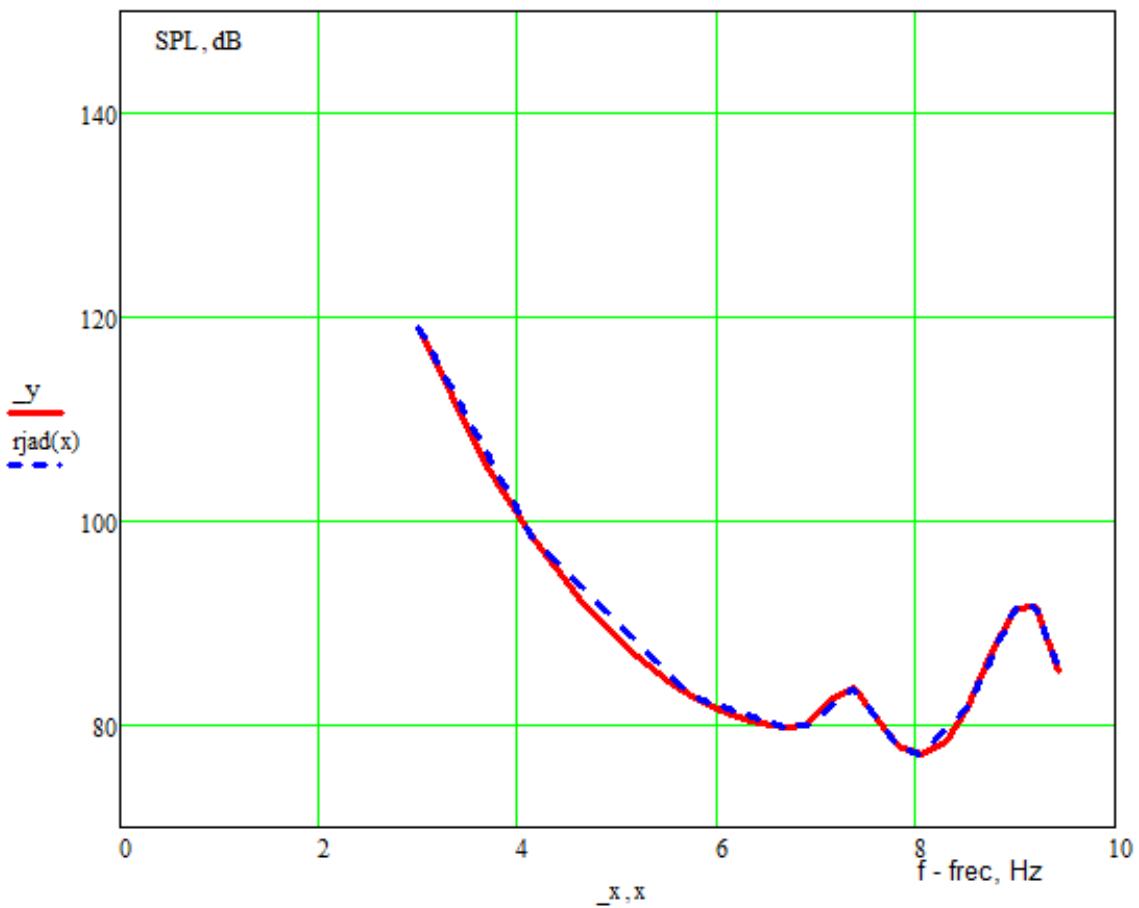 Figure 9: Curves of equal loudness $y$, $dB$ and a curve approximating them $rjad(x)$, Hertz From the materials presented in the figures, it can be seen that for a given number of points, the approximation is satisfactory. ## IV. CONCLUSIONS Differential integral functions, this is the Riemann-Liouville differential integral, written in a convenient form, as a function of two variables[^7]: the usual argument $x$ and the parameter $k$, which sets the multiplicity of the integral or the order of the derivative. These functions allow you to calculate the desired integral or derivative by substituting the parameter $k$ into the established formula. The formula does not change, only one parameter changes. Classical tables of integrals and differentials are not required. Only tables of pre-prepared formulas of differential functions are used, which can be represented in simple calculations in the form of icons, and in the form of SL ( $x$, $k$ ) functions in computer programs written in programming languages such as VBasic, C++, Excel, MathCad, Python, etc. These differential integral functions are of great practical importance, for example, they allow us to approximate a certain given function in the vicinity of the desired point (by the type of decomposition into a Taylor, Maclaurin, Fourier series or $Z$ transformation) or on a segment. At the same time, the conditions of equality of not only the function itself, but also the selected derivatives and differentials, integer and fractional, are observed at the desired approximation points themselves. Examples of approximation of some elementary functions are shown, for example, using a standard polynomial. It is also possible to approximate trigonometric, power functions and their combinations. To simplify working with differential integral functions, they can be represented in two forms: for a graphic image-as a function with angle brackets, and for writing in the program text-as a function $SL(x, k)$ of two or more arguments (Application B). ### APPLICATION A $$ k _ {-} 1 := 1 + 1 \cdot 1 0 ^ {- 6} \quad \mathrm {S L} (\mathrm {x}, \mathrm {k}, \mathrm {n}) := \frac {\mathrm {x} ^ {\mathrm {n} - \mathrm {k}} \cdot \Gamma (\mathrm {n} + 1)}{\Gamma (\mathrm {n} - \mathrm {k} + 1)} \quad \begin{array}{c} \text {T h e s e t p o i n t -} \mu \\\mu := 3 \end{array} $$ $$ \begin{array}{l l}k = 0&\dashrightarrow\\k = 0, 2 5&\dashrightarrow\\k = 0, 5 0&\dashrightarrow\\k = 0, 7 5&\dashrightarrow\\k = 1, 0 0&\dashrightarrow\\k = 1, 2 5&\dashrightarrow\end{array}\quad A 1 := \left( \right.\begin{array}{c c c c c c}1&\mu&\mu^ {2}&\mu^ {3}&\mu^ {4}&\mu^ {5}\\\frac {\mu^ {- 0 . 2 5} \cdot \Gamma (1)}{\Gamma (1 - 0 . 2 5)}&\frac {\mu^ {1 - 0 . 2 5}}{\Gamma (2 - 0 . 2 5)}&\frac {2 \cdot \mu^ {2 - 0 . 2 5}}{\Gamma (3 - 0 . 2 5)}&\frac {6 \cdot \mu^ {3 - 0 . 2 5}}{\Gamma (4 - 0 . 2 5)}&\frac {2 4 \cdot \mu^ {4 - 0 . 2 5}}{\Gamma (5 - 0 . 2 5)}&\frac {1 2 0 \cdot \mu^ {5 - 0 . 2 5}}{\Gamma (6 - 0 . 2 5)}\\\frac {\mu^ {- 0 . 5} \cdot \Gamma (1)}{\Gamma (1 - 0 . 5)}&\frac {\mu^ {1 - 0 . 5}}{\Gamma (2 - 0 . 5)}&\frac {2 \cdot \mu^ {2 - 0 . 5}}{\Gamma (3 - 0 . 5)}&\frac {6 \cdot \mu^ {3 - 0 . 5}}{\Gamma (4 - 0 . 5)}&\frac {2 4 \cdot \mu^ {4 - 0 . 5}}{\Gamma (5 - 0 . 5)}&\frac {1 2 0 \cdot \mu^ {5 - 0 . 5}}{\Gamma (6 - 0 . 5)}\\\frac {\mu^ {- 0 . 7 5} \cdot \Gamma (1)}{\Gamma (1 - 0 . 7 5)}&\frac {\mu^ {1 - 0 . 7 5}}{\Gamma (2 - 0 . 7 5)}&\frac {2 \cdot \mu^ {2 - 0 . 7 5}}{\Gamma (3 - 0 . 7 5)}&\frac {6 \cdot \mu^ {3 - 0 . 7 5}}{\Gamma (4 - 0 . 7 5)}&\frac {2 4 \cdot \mu^ {4 - 0 . 7 5}}{\Gamma (5 - 0 . 7 5)}&\frac {1 2 0 \cdot \mu^ {5 - 0 . 7 5}}{\Gamma (6 - 0 . 7 5)}\\\frac {\mu^ {- k _ {-} , 1} \cdot \Gamma (1)}{\Gamma (1 - k _ {-} , 1)}&\frac {\mu^ {1 - 1}}{\Gamma (2 - 1)}&\frac {2 \cdot \mu^ {2 - 1}}{\Gamma (3 - 1)}&\frac {6 \cdot \mu^ {3 - 1}}{\Gamma (4 - 1)}&\frac {2 4 \cdot \mu^ {4 - 1}}{\Gamma (5 - 1)}&\frac {1 2 0 \cdot \mu^ {5 - 1}}{\Gamma (6 - 1)}\\\frac {\mu^ {- 1 . 2 5} \cdot \Gamma (1)}{\Gamma (1 - 1 . 2 5)}&\frac {\mu^ {1 - 1 . 2 5}}{\Gamma (2 - 1 . 2 5)}&\frac {2 \cdot \mu^ {2 - 1 . 2 5}}{\Gamma (3 - 1 . 2 5)}&\frac {6 \cdot \mu^ {3 - 1 . 2 5}}{\Gamma (4 - 1 . 2 5)}&\frac {2 4 \cdot \mu^ {4 - 1 . 2 5}}{\Gamma (5 - 1 . 2 5)}&\frac {1 2 0 \cdot \mu^ {5 - 1 . 2 5}}{\Gamma (6 - 1 . 2 5)}\end{array} $$ $$ \mathrm {B} 1 := \left( \begin{array}{l l} \cos \left(\mu + 0.00 \cdot \frac {\pi}{2}\right) & \mathrm {a} := \mathrm {A} 1 ^ {-1} \cdot \mathrm {B} 1 \\ \cos \left(\mu + 0.25 \cdot \frac {\pi}{2}\right) & \underline {{\cos (\mathrm {x})}} := \mathrm {a} _ {0} + \mathrm {a} _ {1} \cdot \mathrm {x} + \mathrm {a} _ {2} \cdot \mathrm {x} ^ {2} + \mathrm {a} _ {3} \cdot \mathrm {x} ^ {3} + \mathrm {a} _ {4} \cdot \mathrm {x} ^ {4} + \mathrm {a} _ {5} \cdot \mathrm {x} ^ {5} \\ \cos \left(\mu + 0.50 \cdot \frac {\pi}{2}\right) & -0.5 \\ \cos \left(\mu + 0.75 \cdot \frac {\pi}{2}\right) & -1 \\ \cos \left(\mu + 1.00 \cdot \frac {\pi}{2}\right) & -1.5 \\ \cos \left(\mu + 1.25 \cdot \frac {\pi}{2}\right) & -2 \\ & x \\ & -9.899925 \times 10^{-1} \\ & -9.899925 \times 10^{-1} \\ & -9.899925 \times 10^{-1} \\ & -9.899925 \times 10^{-1} \\ & -9.899925 \times 10^{-1} \\ & -9.899925 \times 10^{-1} \\ & -9.899925 \times 10^{-1} \\ & -9.899925 \times 10^{-1} \\ & -9.899925 \times 10^{-1} \\ & -9.899925 \times 10^{-1} \\ & -9.899925 \times 10^{-1} \\ & -9.899925 \times 10^{-1} \\ & -9.899925 \times 10^{-1} \\ & -9.899925 \times 10^{-1} \\ & -9.899925 \times 10^{-1} \\ & -9.899925 \times 10^{-1} \\ & -9.899925 \times 10^{-1} \\ & -9.899925 \times 10^{-1} \\ & -9.899925 \times 10^{-1} \\ & -9.899925 \times 10^{-1} \\ & -9.899925 \times 10^{-1} \\ & -9.899925 \times 10^{-1} \\ & -9.899925 \times 10^{-1} \\ & -9.899925 \times 10^{-1} \\ & -9.899925 \times 10^{-1} \\ & -9.899925 \times 10^{-1} \\ & -9.899925 \times 10^{-1} \\ & -9.899925 \times 10^{-1} \\ & -9.899925 \times 10^{-1} \\ & -9.899925 \times 10^{-1} \\ & -9.899925 \times 10^{-1} \\ & -9.899925 \times 10^{-1} \\ & -9.899925 \times 10^{-1} \\ & -9.899925 \times 10^{-1} \\ & -9.899925 \times 10^{-1} \\ & -9.899925 \times 10^{-1} \\ & -9.899925 \times 10^{-1} \\ & -9.899925 \times 10^{-1} \\ & -9.899925 \times 10^{-1} \\ & -9.899925 \times 10^{-1} \\ & -9.899925 \times 10^{-1} \\ & -9.899925 \times 10^{-1} \\ & -9.899925 \times 10^{-1} \\ & -9.899925 \times 10^{-1} \\ & -9.899925 \times 10^{-1} \\ & -9.899925 \times 10^{-1} \\ & -9.899925 \times 10^{-1} \\ & -9.899925 \times 10^{-1} \\ & -9.899925 \times 10^{-1} \\ & -9.899925 \times 10^{-1} \\ & -9.899925 \times 10^{-1} \\ & -9.899925 \times 10^{-1} \\ & -9.899925 \times 10^{-1} \\ & -9.899925 \times 10^{-1} \\ & -9.899925 \times 10^{-1} \\ & -9.899925 \times 10^{-1} \\ & -9.899925 \times 10^{-1} \\ & -9.899925 \times 10^{-1} \\ & -9.899925 \times 10^{-1} \\ & -9.899925 \times 10^{-1} \\ & -9.899925 \times 10^{-1} \\ & -9.899925 \times 10^{-1} \\ & -9.899925 \times 10^{-1} \\ & -9.899925 \times 10^{-1} \\ & -9.899925 \times 10^{-1} \\ & -9.899925 \times 10^{-1} \\ & -9.899925 \times 10^{-1} \\ & -9.899925 \times 10^{-1} \\ & -9.899925 \times 10^{-1} \\ & -9.899925 \times 10^{-1} \\ & -9.899925 \times 10^{-1} \\ & -9.899925 \times 10^{-1} \\ & -9.899925 \times 10^{-1} \\ & -9.899925 \times 10^{-1} \\ & -9.899925 \times 10^{-1} \\ & -9.899925 \times 10^{-1} \\ & -9.899925 \times 10^{-1} \\ & -9.899925 \times 10^{-1} \\ & -9.899925 \times 10^{-1} \\ & -9.899925 \times 10^{-1} \\ & -9.899925 \times 10^{-1} \\ & -9.899925 \times 10^{-1} \\ & -9.899925 \times 10^{-1} \\ & -9.899925 \times 10^{-1} \\ & -9.899925 \times 10^{-1} \\ & -9.899925 \times 10^{-1} \\ & -9.899925 \times 10^{-1} \\ & -9.899925 \times 10^{-1} \\ & -9.899925 \times 10^{-1} \\ & -9.899925 \times 10^{-1} \\ & -9.899925 \times 10^{-1} \\ & -9.899925 \times 10^{-1} \\ & -9.899925 \times 10^{-1} \\ & -9.899925 \times 10^{-1} \\ & -9.899925 \times 10^{-1} \\ & -9.899925 \times 10^{-1} \\ & -9.899925 \times 10^{-1} \\ & -9.899925 \times 10^{-1} \\ & -9.899925 \times 10^{-1} \\ & -9.899925 \times 10^{-1} \\ & -9.899925 \times 10^{-1} \\ & -9.899925 \times 10^{-1} \\ & -9.899925 \times 10^{-1} \\ & -9.899925 \times 10^{-1} \\ & -9.899925 \times 10^{-1} \\ & -9.899925 \times 10^{-1} \\ & -9.899925 \times 10^{-1} \\ & -9.899925 \times 10^{-1} \\ & -9.899925 \times 10^{-1} \\ & -9.899925 \times 10^{-1} \\ & -9.899925 \times 10^{-1} \\ & -9.899925 \times 10^{-1} \\ & -9.899925 \times 10^{-1} \\ & -9.899925 \times 10^{-1} \\ & -9.899925 \times 10^{-1} \\ & -9.899925 \times 10^{-1} \\ & -9.899925 \times 10^{-1} \\ & -9.899925 \times 10^{-1} \\ & -9.899925 \times 10^{-1} \\ & -9.899925 \times 10^{-1} \\ & -9.899925 \times 10^{-1} \\ & -9.899925 \times 10^{-1} \\ & -9.899925 \times 10^{-1} \\ & -9.899925 \times 10^{-1} \\ & -9.899925 \times 10^{-1} \\ & -9.899925 \times 10^{-1} \\ & -9.899925 \times 10^{-1} \\ & -9.899925 \times 10^{-1} \\ & -9.899925 \times 10^{-1} \\ & -9.899925 \times 10^{-1} \\ & -9.899925 \times 10^{-1} \\ & -9.899925 \times 10^{-1} \\ & -9.899925 \times 10^{-1} \\ & -9.899925 \times 10^{-1} \\ & -9.899925 \times 10^{-1} \\ & -9.899925 \times 10^{-1} \\ & -9.899925 \times 10^{-1} \\ & -9.899925 \times 10^{-1} \\ & -9.899925 \times 10^{-1} \\ & -9.899925 \times 10^{-1} \\ & -9.899925 \times 10^{-1} \\ & -9.899925 \times 10^{-1} \\ & -9.899925 \times 10^{-1} \\ & -9.899925 \times 10^{-1} \\ & - Figure A.1: Decomposition of the function $\cos(x)$ into a series $\cos(x)$ in the vicinity of two different points $\mu = 3$ and $\mu = 15$ The system consists of the polynomial $\cos(x)$ and its six fractional derivatives $k_i$, with a maximum multiplicity of 1.25. The order of the derivatives of $k$ changes after 0.25. ## APPLICATION B Differential integral functions of $\mathsf{SL}(.)$ The text of the VBasic program for calculating the differential functions of SL() is given below. The text of the program in VBasic for calculating the differential functions of SL(). Option Explicit Dim n, k As Double $$ Dim in_n, in_k As Double $$ ## Dim Message1, Title1, Default, MyValue ## Dim Message2, Title2 ## Dim MathcadObj ## Dim MCWSheet $$ Private Sub Form_Load() $$ Form1.Enabled = True Form1.Cls Form1.Visible = False Form1 Appearance = 0 Form1.WhenState $= 2$ Callnk End Sub Private Sub nk() Message1 = "Enter the degree <n> for the power function y = x^n" $$ Title1 = "Default n = 2" $$ Default $=$ "2" MyValue = InputBox (Message1, Title1, Default) n = CDbl (MyValue) Message2 = ""Enter K. If K < 0, then it is an integral of multiplicity K, and if K > 0, then it is a derivative of order K". k = InputBox (Message2, Title1, Default) Call Gam End Sub Private Sub Gam() Setting a custom function Set MathcadObj = OLE1(object Set MCWSheet = MathcadObj.Worksheet in $n = n$ in $k = k$ $$ Call MathcadObj.setcomplex("in_n", n, 0) $$ $$ Call MathcadObj.setcomplex("in_K", k, 0) $$ Recalculating results in MathCad and getting a custom SLFunctions function Call MathcadObj.Recalculate 'End of the program DimMsg,Style,Title,Response Msg = "Continue? Yes" Style = vbYesNo + vbCritical + vbDefaultButton2 Title = "The program has finished working. Viewing the result" Response = MsgBox (Msg, Style, Title) If Response = 6 Then Form1.Enabled = False Set MathcadObj = Nothing Set MCWSheet = Nothing End End Sub Below, as an example, is a table (Table 1) with the results of calculating the differential functions on VBasic, where n is the exponent of the power function, and k is the parameter of the differential function. For $k < 0$ it is a fractional integral, $k = 0$ is the parent function, and for $k > 0$ it is a fractional derivative. Table B.1: Values of functions ${x}^{0,{123}},{x}^{2},{x}^{{12},3}$ and $\sin \left(x\right)$ <table><tr><td>PDF File</td><td>n</td><td>k</td><td colspan="2">Figure</td></tr><tr><td rowspan="4">(0,123) &lt;-1,93&gt;Fractionalintegral 1.1SLFunction n=0,123k=-1,93.pdf</td><td rowspan="4">0,123</td><td rowspan="4">-1,93</td><td>n = in_n n = 0.123k:= in_k k = -1.93KG(n,k):= Γ(n+1)/Γ(n+1-k) y(x,n,k):= kG(n,k) x^n(k)</td><td>nk(n,k):= n - ky(x,n,k) float, 3 → 0.448 x2.05</td></tr><tr><td>y(x,n,k)</td><td>60</td></tr><tr><td>-10</td><td>-5</td></tr><tr><td>x</td><td>5</td></tr><tr><td rowspan="4">0,123 &lt;0&gt;Maternalfunction No.1SLFunction n=0,123k=0.pdf</td><td rowspan="4">0,123</td><td rowspan="4">0</td><td>n = in_n n = 0.123k:= in_k k = 0kG(n,k):= Γ(n+1)/Γ(n+1-k) y(x,n,k):= kG(n,k) x^n(k)</td><td>nk(n,k):= n - ky(x,n,k) float, 3 → 1.0 x0.123</td></tr><tr><td>y(x,n,k)</td><td>1.5</td></tr><tr><td>-10</td><td>-5</td></tr><tr><td>x</td><td>5</td></tr><tr><td rowspan="2">(0,123)&lt;0,37&gt;Fractionalderivative1.1SLFunction n=1,234k=0,37.pdf</td><td rowspan="2">0,123</td><td rowspan="2">0,37</td><td>n:=in_n n=1.234k:=in_k k=0.37kG(n,k)= Γ(n+1)/ Γ(n+1-k) y(x,n,k)=kG(n,k)-x nk(n,k)</td><td>nk(n,k):= n - ky(x,n,k) float, 3 → 1.18 · x0.864</td></tr><tr><td>y(x,n,k)</td><td>10/8-10-50-510</td></tr><tr><td rowspan="2">2&lt;-&gt;The two-foldintegral2.1PDFSLFunction n=2k=-2.pdf</td><td rowspan="2">2</td><td rowspan="2">-2</td><td>n:=in_n n=2k:=in_k k=-2kG(n,k)= Γ(n+1)/ Γ(n+1-k) y(x,n,k)=kG(n,k)-x nk(n,k)</td><td>nk(n,k):= n - ky(x,n,k) float, 3 → 0.0833 · x4</td></tr><tr><td>y(x,n,k)</td><td>1×103800600400200x</td></tr><tr><td rowspan="2">2&lt;-1.64&gt;Fractionalintegral 2.2SLFunction n=2k=-1.64.pdf</td><td rowspan="2">2</td><td rowspan="2">-1,64</td><td colspan="2">n:=in_n n=2k:=in_k k=-1.64kG(n,k):=Γ(n+1)/Γ(n+1-k)nk(n,k):=n-ky(x,n,k)=KG(n,k)-xnk(n,k) y(x,n,k) float,3→0.141-x3.64</td></tr><tr><td>y(x,n,k)</td><td>800600400200x</td></tr><tr><td rowspan="2">2&lt;-1&gt;Singleintegral 2.3SLFunction n=2k=-1.pdf</td><td rowspan="2">2</td><td rowspan="2">-1</td><td colspan="2">n:=in_n n=2k:=in_k k=-1kG(n,k):=Γ(n+1)/Γ(n+1-k)nk(n,k):=n-ky(x,n,k)=KG(n,k)-xnk(n,k) y(x,n,k) float,3→0.333-x3</td></tr><tr><td>y(x,n,k)</td><td>400200x</td></tr><tr><td rowspan="5">2&lt;0&gt;Maternal functionNo.2 PDF SLFunction n=2 k=0.pdf</td><td rowspan="5">2</td><td rowspan="5">0</td><td>n:=in_n n=2 k:=in_k k=0 kG(n,k):= Γ(n+1)/ Γ(n+1-k) y(x,n,k):= kG(n,k)-x nk(n,k)</td><td>nk(n,k):= n-k y(x,n,k) float,3→x2</td></tr><tr><td>y(x,n,k)</td><td>100/80/60/40/20/5/10</td></tr><tr><td>-10</td><td>-5</td></tr><tr><td>0</td><td>5</td></tr><tr><td>x</td><td>10</td></tr><tr><td rowspan="6">2&lt;1&gt; The firstderivative 2.1 PDF SLFunction n=2 k=1.pdf</td><td rowspan="6">2</td><td rowspan="6">1</td><td>n:=in_n n=2 k:=in_k k=1 kG(n,k):= Γ(n+1)/ Γ(n+1-k) y(x,n,k):= kG(n,k)-x nk(n,k)</td><td>nk(n,k):= n-k y(x,n,k) float,3→2.0-x</td></tr><tr><td>y(x,n,k)</td><td>20/10/10/5/10</td></tr><tr><td>-10</td><td>-5</td></tr><tr><td>0</td><td>5</td></tr><tr><td>-10</td><td>-20</td></tr><tr><td>x</td><td>10</td></tr><tr><td rowspan="4">2&lt;1,75&gt;Fractionalderivative 2.2SLFunction n=2k=1,75.pdf</td><td rowspan="4">2</td><td rowspan="4">1,75</td><td>n:=in_n n=2k:=in_k k=1.75kG(n,k)= Γ(n+1)/ Γ(n+1-k) y(x,n,k)=kG(n,k)-nk(n,k)</td><td>nk(n,k)=n-ky(x,n,k) float,3→2.21·x0.25</td></tr><tr><td>y(x,n,k)</td><td>y(x,n,k) float,3→2.21·x0.25</td></tr><tr><td>-10</td><td>-5</td></tr><tr><td>x</td><td>10</td></tr><tr><td rowspan="6">2&lt;2&gt; The secondderivative 2.3 PDFSLFunction n=2k=2.pdf</td><td rowspan="6">2</td><td rowspan="6">2</td><td>n:=in_n n=2k:=in_k k=2kG(n,k)= Γ(n+1)/ Γ(n+1-k) y(x,n,k)=kG(n,k)-nk(n,k)</td><td>nk(n,k)=n-ky(x,n,k) float,3→2.0</td></tr><tr><td>y(x,n,k)</td><td>2.002</td></tr><tr><td>2.001</td><td>2.001</td></tr><tr><td>1.999</td><td>1.999</td></tr><tr><td>-10</td><td>-5</td></tr><tr><td>x</td><td>10</td></tr></table> <table><tr><td>(12,34)&lt;-0.45&gt;Fractional integral 3.1SL Fun 12,34-0,45.xmcd</td><td>12,34</td><td>-0,45</td><td>BveiTe nokazatelb stelenhnof yunkuni&lt; n &gt;n:= 12.34BveiTe noprajdoK npoizBODnoi iIinnterpala &lt; k &gt;ДяnpoizBODnoi k &gt; 0 dnia nnterpala k &lt; 0k:= -0.45ДиферитральногФункuniya ravhay(x,n,k):= Γ(n+1)/Γ(n+1-k)x-n-ky(x,n,k) float,3 → 0.315-x12.8Bvnd этой phункuni рedingставен на графпке</td></tr><tr><td>12,34&lt;0-MaternalfunctionNo.3SL Fun 12,34 0.xmcd</td><td>12,34</td><td>0</td><td>BveiTe nokazatelb stelenhnof yunkuni&lt; n &gt;n:= 12.34BveiTe noprajdoK npoizBODnoi iIinnterpala &lt; k &gt;ДяnpoizBODnoi k &gt; 0 dnia nnterpala k &lt; 0k:= 0ДиферитральногФункuniya ravhany(x,n,k):= Γ(n+1)/Γ(n+1-k)x-n-ky(x,n,k) float,3 → 1.0-x12.3Bvnd этой phункuni рedingставen на графпке</td></tr><tr><td>(12,34)&lt;1,75&gt;Fractionalderivative3.1SL Fun 12,341,75.xmcd</td><td>12,34</td><td>1,75</td><td>BveiTe poka3aTeIb cTepeHNo fynKznn &lt; n &gt;n:= 12,34BveiTe nopiaOk npoi3BODnoi iIinnterpana &lt; k &gt;Дяnpoi3BODnoi k &gt; 0 dIyIINTErpana k &lt; 0k:= 1,75ДифериNTerpaIbnaФункшу Y parBa y(x,n,k):= Γ(n+1)/Γ(n+1-k)x-n-ky(x,n,k) float,3→76.9x10.6BvIэTofynKznnпstablenHa rpaФиke</td></tr><tr><td>sin(x)&lt;1,64&gt;Fractionalintegral4.1PDEsin x -1,64.pdf</td><td></td><td>-1,64</td><td>BveiTe nopiaDok npoi3BODnoi iIinnterpana &lt; k &gt;Дяnpoi3BODnoi k &gt; 0 dIyIINTErpana k &lt; 0k:= -1,64ДифериNTerpaIbnaФункшу Y parBa y(x,k):= sin(x+k/2)y(x,k) float,3→sin(x-2.58)BvIэTofynKznnпstablenHa rpaФиke</td></tr><tr><td>sin(x) &lt;0&gt;Maternal function No.4PQFsin x 0.pdf</td><td></td><td>0</td><td>BVeДиTe nopяДоК п ropИЗВODнОй илі міnteграпа &lt; k &gt;Дя п ropИЗВODнОй k &gt; 0 дя міntegerралa k &lt; 0k:0ДиФ�ериNTergральнай Функшу Y parhay(x,k) sin(x+k-π/2)y(x,k) float,3→sin(x)Вid зтой phунцшп рedingставен на графиke</td></tr><tr><td>sin(x) &lt;1.75&gt;Fractionalderivative4.1PQFsin x 1,75.pdf</td><td></td><td>1,75</td><td>ВveДиTe nopяДоК п ropИЗВODнОй илі міnteграпа &lt; k &gt;Дя п ropИЗВODнОй k &gt; 0 дя міntegerралa k &lt; 0k:1,75ДиФ�ериNTergральнай Функшу Y parhay(x,k) sin(x+k-π/2)y(x,k) float,3→sin(x+2.75)Вid зтой phунцшп рedingставен на графиke</td></tr></table> [^1]: And also, definitions of derivatives/integrals based on such concepts as the Riemann-Liouville, Grunwald-Letnikov and Weyl differentialintegrals. _(p.1)_ [^2]: Here $SL(x,k)$ is another form of writing a power differential function, different from writing the formy _(p.5)_ [^3]: Here and further calculations are performed in the MathCad program, so it uses a dot in its formulas instead of a comma. _(p.5)_

Generating HTML Viewer...

References

15 Cites in Article
V Vladimirov (1974). Statement of Boundary Value Problems in Mathematical Physics.
A Tikhonov,A Samarsky (1999). Equations of mathematical physics: Textbook. Manual.
V Vladimirov,A Vasharin,H Karimova,V Mikhailov (1986). A Collection of Problems on the Equations of Mathematical Physics.
V Vladimirov Equations of mathematical physics.
V Vladimirov,E Kutafina (2004). Exact travelling wave solutionsof some nonlinear evolutionary equations.
Mikusinsky Yan (2006). Operational Calculus.
V Martynenko (1990). Operational calculus.
Sidorov Yu,M Fedoryuk,M Shabunin Lectures on the theory of functions of a complex variable: Textbook for universities--3rd.
Gustav Dech Guide to practical application of the Laplace transform and Z-transform.
V Ditkin,A Prudnikov (1959). Operational calculus in two variables and its applications.
A Lykov (2016). Thermal Conductivity: Thermal Conductivity of Nanouids in Stationary and Dynamic Systems.
B Voronenko,A Krysin,V Pelenko,O Tsuranov (2014). Analytical description of the process of non-stationary thermal conductivity.
K Bukhensky,N Maslova (1975). APPLICATION OF OPERATIONAL CALCULUS FOR THE DESCRIPTION OF TRANSIENT PROCESSES IN ELECTRICAL CIRCUITS.
R Shostak,Ya (1972). Operational calculus.
I Zolotarev (2004). Application of the method simplifying the inverse Laplace transform in the study of the dynamics of oscillatory systems.
No ethics committee approval was required for this article type.
Data Availability
Not applicable for this article.
How to Cite This Article
Alexey S. Dorokhov. 2026. \u201cApplication of Differentialintegral Functions\u201d. Global Journal of Research in Engineering - I: Numerical Methods GJRE-I Volume 23 (GJRE Volume 23 Issue I1).
Explore published articles in an immersive Augmented Reality environment. Our platform converts research papers into interactive 3D books, allowing readers to view and interact with content using AR and VR compatible devices.
Your published article is automatically converted into a realistic 3D book. Flip through pages and read research papers in a more engaging and interactive format.
Our website is actively being updated, and changes may occur frequently. Please clear your browser cache if needed. For feedback or error reporting, please email [email protected]
Thank you for connecting with us. We will respond to you shortly.