## I. INTRODUCTION The Pharmaceutical industry in India is the third largest in the world in terms of volume and 14th largest in terms of value. It is one of the top five sectors contributing to foreign exchange earnings and provides employment to over 2.7 million people thus playing a major role in the Indian economy. It contributes around $1.72\%$ of the country's GDP. The size of the industry is USD 50 Bn. (2020-21) and contributes a net annual trade surplus of USD 17 Bn. India's revenue from pharmaceutical exports was $25.3 billion in the 2022-2023 financial year. In terms of the global market, India currently holds a significant share of the world market and is known as the Pharmacy of the World. According to a recent EY FICCI report, that the Indian pharmaceutical market is estimated to reach $ 65 Bn. in 2024 & is estimated to touch US$ 130 billion in value by the end of 2030.To achieve this milestone, the need for funds in the pharmaceutical industry is huge and has to be procured either as owners' equity or borrowed funds. Whether to use owners' equity or resort to debt funds is a very crucial financial decision to be taken by the financial manager of the pharmaceutical company. Generally, companies use both debt capital and equity capital with varying proportions in their debt equity mix. Theoretically it is contented that the companies can use debt equity mix in a manner that enhances returns to its shareholders. There is a conflict as to the relevance of debt in the maximisation of shareholders' value. This controversial situation has given birth to different theories of capital structure but none of them is flawless, as they suffer from various limitations and cannot be viewed as valid proportions applicable in all situations. The relevant school of thought dominated by Prof. Durand (1952), has contended that use of debt with an equity influences cost of capital, thereby there exists an optimum capital structure. Contrary to this, the irrelevant school of thought dominated by Modigliani & Miller (1958) on the basis of their empirical study have hypothesed that within the framework of perfect Capital Markets and in the absence of corporate taxes & bankruptcy costs, there does not exist an Optimum - Capital Structure. These & several other questions related to the Capital Structure decisions remains perplexing because of diverse & conflicting theories & also due to diverse empirical results. [Abdul Aziz et al (2015), Raluca-Georgiana MOSCU (2014)]. These conflicting views overshadow the impact of financial leverage on firm performance. The fact is that no general consensus has yet emerged even after several decades of investigation [Julius Bitok et al (2011)]& scholars can be found often disagreeing even about the same empirical evidence. [Kale, A. A. (2014)]. These& other factors have made the researchers to continuously investigate into this crucial aspect of corporate financial decision making aspect. [Lucy Wamugoet al (2014)]. The capital structure decision is critical decision for any organization. The decision is important not only because of the need to maximize returns to its stockholders, but also because of the impact such a decision has on an organization's survival & growth in today's competitive environment [ Dare Funso David et al (2010)]. Its added importance is, because a faulty capital structure decision can have both micro & macroeconomic implications, as remarked by Julius Bitok (2011), "Throughout the history most of the world's most severe financial crises have had their causes traced to the poor Management of debt". The financial distress in the Real Estate Business commonly known as "Bursting of Housing Bubble", which resulted in the Global recession of 2007-2009 can be cited in support for the same. Financial decision is thus very crucial for the Financial well-being of a firm itself [Catherine Warue Njagi (2013)] as well as general economy. It is therefore, imperative for the financial Manager to have a clear understanding of this financial decision so that they can take right decision at right time, leading thereby to optimal debt-equity mix, which is really a formidable task. For this purpose, one has to go beyond theory [Gowri- M. K. (2013). While some scholars have found positive relation between debt financing and Firm performance, others have revealed an inverse relationship between the two. Some, studies even concluded that the relationship between capital structure & Firm performance is both positive & negative [Tsangaav et al (2009), Oke & Afolabi (2008) - khalaf Tanni (2013)]. Still other researchers established empirically that there isn't any significant relationship between C/S & Firm Performance. [Soni. B, Trividi J. (2014) Ibrahim (2009)]. Though, extensive studies have been made in this regard, still no unified theory has come out, which could have derived the major support, thus leaving the subject open for further research. [Handoo. A & Sharma K. (2014)]. Like other sectors, the Impact of financial leverage on the firm performance in the pharmaceutical sector has also been assessed in various countries including India. However, impact of financial leverage on financial performance of a firm under different economic conditions has not been ascertained. More so, research works have taken the average total debt of low, average & high debt companies of the sector. But this study is restricted to only the high debt companies of the sector so as to determine the impact of high debt on the financial performance of a firm. ## II. LITERATURE REVIEW Capital Structure is most debated topics within the area of corporate finance. It derives its importance from the fact that, an appropriate Capital Structure is not only essential for the firm itself, but it has also micro & macro-economic implications. It is because of this significance, that a large number of theoretical as well as empirical studies in this field have emerged over the last few decades, with shifting paradigm from market economies to transitional economies, from developed economies to developing economies, from country-based studies to regional studies. The literature on capital structure is theoretical as well as empirical. Of the various theories of Capital Structure, "The Traditional Relevance Theory" of Prof. Durand (1952) and the "Modern Irrelevance Theory" of Modigliani & Miller (1958) are the main theories both focussing on the relationship between Capital Structure & the firm performance. Out of the various prepositions on Financial Leverage regarding proportion of debt in the Capital Structure, the two extreme views are Net income approach & Net Operating Income approach [Prof. Durand (1952)], besides an intermediate approach known as the traditional. As per Net income approach, the Weighted Average Cost of Capital (WACC) decreases by including debt funds in the Capital Structure & thus the value of firm increases. However, the Net Operating income approach holds an opposite view of it. As per this approach, the overall cost of capital is independent of the financial leverage. This is based on the assumption that the cost of equity increases linearly with increase in leverage, such that the overall cost of the capital remains the same. In between these two extreme view, is the intermediate or traditional approach of Solomon (1963) Which argues that the cost of capital declines & the value of firm increases with the increase in financial leverage up to a prudent debt level- the optimum point. Thereafter with increase in the debt content in the capital structure, there is an increase in WACC which in turn has a negative impact on value of firm. The irrelevance theory of capital structure is supported by many Scholars Stighitz, (1969), Baron (1974), Stighitz (1974) Schneller (1980) & Taggart (1977). Whereas the traditional approach - which can be described as a modified version of Net income approach, is in line with what is referred to as relevancy theory of Capital Structure and has many empirical backing apart from models & hypothesis in its support. Morten (1954), Lutiner (1956), Kim (1978) Haugen & Senbet (1978) Marsh (1982) & Ozkan (2001) second this view point. A number of studies have been carried out on Capital Structure both in India & abroad. These studies have debated on different aspects of Corporate Capital Structure viz. relationship between Capital Structure decisions and cost of Capital, determinants of Capital Structure, Impact of Financial Leverage on EPS, ROI, ROE & Value of firm. In order to get the right perspective of the different aspects of Capital Structure decision, it is in the fitness of the things to have a brief review of important studies conducted so far. The modern theory of Capital Structure began with the classical paper by Modigliani & Miller (1958) which posit that under perfect Capital Market conditions & in the absence of corporate taxes & bankruptcy costs, financing decision has no bearing on the company's composite cost of Capital and Value of firm. In favour of their thesis, they have held that the Value of firm depends on earning power of a firm which in turn depends upon the Investment decision. A number of studies like Bhandari (1988), Hecht (2000), Lasfer (1995) & Boothetal (2001) held similar views on the relationship between Financing decision & Value of firm. However, there are equally large number of studies which have challenged the relevance of M - M theorem & have suggested that a relationship between Financial Leverage & Corporate performance does exist. For example, Arditi (1967) on the basis of his study has found a negative but statistically insignificant relationship between financial leverage & equity returns. The inverse relationship between financial leverage & equity returns has also been found by Hovakimian et. al (2001), Hamada (1972) & Dimtrov & Jain (2008). Further, Sharma & Roa (1968) on the basis of their study have found that the leverage variable had a coefficient greater than the tax rate, thus falls in line with the traditional view that the cost of capital is affected by debt apart from its tax advantage. The studies of Panday (1981) & Ward & Price (2006) have also supported the traditional view in the sense that there exists a relationship between the levels of financial leverage & cost of capital. Some experts are of the view that Capital Structure & Profitability have strong relationship with each other. According to interest – tax shield hypothesis, which is derived from M – M Hypothesis (1963) firms with high profits would employ high debt to gain tax benefits. On the contrary, Pecking Order of financing or asymmetric information hypothesis of Myres & Majluf (1984) postulates that the companies with higher profitability prefer internal financing. De Angelo & Masulis (1980) findings have been in conformity with the asymmetric information hypothesis & have also found that the interest – tax shield hypothesis may also not work in those firms that have other than interest tax shield avenues like depreciation. No unanimity has been found in the empirical evidences regarding the relationship between the Capital Structure and firm performance. Positive, negative as well as mixed relationship is revealed by the research conducted by various scholars. Sharma (2006) & Kuben Reyan (2008) has found direct relation between leverage and firm value. Similar view has been held by Lasher (2016) when he asserts that increased level of debt finance can result in increased earnings per share and return on equity. Dewet (2006) proved that a significant increase in value of firm can be achieved in moving close to the optimal level of gearing. Fama & French (2010) seconded him, when they concluded that there should be a positive relation between debt ratio and firm profitability. Positive relationship between total debt and return on equity and total assets has also been reported by Larry & Stulz (1995) in firms in Ghana. Nawaz, Javid & Akhtar (2012) have also reported a positive linkage between capital structure and firm performance. Significant positive relationship between Capital Structure and EPS & financial leverage and return on equity has also been observed by Mubeen & Akhtar (2014) in the firms listed in Karachi Stock Exchange and by Abdul Azeez et al (2015) from Nigerian firms respectively. In consistency with the above findings are the empirical evidences of champion (1999), Gosh et al (2000) HadLock and Jame (2002), Frank and Goyal (2009) and Berger and Bonaccors di patti (2006). But at the same time, no less a number of empirical studies bring out negative impact of financial leverage on firm performance measured in terms of profitability by various proxied ratios Titman & Wessels (1988), Wald (1999) Sheel (1994) Eunju and Soocheong (2005) have reported negative relationship between financial leverage and profitability. Negative Association of financial leverage and firm performance has also been observed by Gleanson et al (2000) Upneja & Dalbor (2001), Deesomsik et al (2004) and Heng (2011); Abu- Rub (2011). Return on equity and debt equity ratio has also been found negatively related in companies in Ghana by Abor (2005), Asian Corporations (Krishnan & Moyer, 1977) North American Region (King & Santor-2008). Shub & Alsawalhah (2012) in Jorden, Ebaid (2009) in Egypt. Lucy Wmage (2014) observed a negative but insignificant relationship between financial leverage and firm performance in Kenya. The research works of various scholars in India have also supported the negative impact of financial leverage on firm performance. Suarabh Chadha, and Sharma A K (2016). Significant negative effect of capital structure on accounting performance has also been reported by Krishna Dayal Panday et al (2019) in Indian manufacturing firms traded on BSE. Similar results have been obtained by Ramachandran Azhagariah et al (2011) in Information Technology Industry in India. However, a positive relation between debt- equity and ROE, D/E and ROA has been reported by Muzumdar D J B in infrastructural companies in India. The findings of Muzumdar were confirmed by Kumar MR (2014) in Bata India Ltd. A study on leverage analysis and profitability for selected paint companies in India by Soni B & Trivedi J (2014) could not find any significant relationship between financial leverage and firm performance measured in terms of profitability. Same is in confirmatory with the findings of Ibrahim (2009). Situation is no different in the case of pharmaceuticals companies, where positive, negative as well as no impact of financial leverage/debt on the firm performance/profitability has been empirically established. While as positive relationship of capital structure and firm financial performance has been evidenced by Hung & Pham (2020) in pharma companies of Vietnam, Shilpi & Dinesh (2016), Prakash & Sindhasha (2016), Mathur et al (2021) and Varghese & Sahai (2021) all reported negative effect of financial leverage on firm performance in Indian Pharma companies. Enekwe et al (2014), Afroze & Ahmed (2022) and Chenxin Zhang (2022) too have found negative relationship between financial leverage and firm performance in Nigeria, Bangladesh and Singapore respectively. However, no link between the financial leverage and capital structure has been documented by Tom Jacob (2020) in the pharma companies of India. As stated by him, "the results indicate that financial leverage has no link with capital structure which proves the Modigliani and Miller theory of capital structure" But Chen, Lecheng. (2023), negates this no link, instead empirically establishes the existence of a link between the company's capital structure and its operating performance, while assessing the impact of capital structure on the operating performance of three listed companies in pharmaceutical industry. Further, he remarks that a reasonable capital structure optimisation can improve a company's operating performance & mitigate operating risk. From the above review of literature, it becomes quite clear that there is lack of unanimity so far as the relationship between the capital structure decision (debt equity ratio) & the firm performance (profitability) is concerned. While some studies point out a positive relationship between the debt equity ratio and profitability, (measured in terms of different proxies), others reveal a negative relationship between the two. Mixed results were also reported by the researchers. McConnell and Servaes (1995) and Agarwal and Zhao (2007) found that in firm with high growth, debt has negative effect on profitability, while firms with low growth effect is positive. ### Hypothesis H1: There is no impact of F/L on payoffs to stockholders of the sample companies. H2: There is an impact of financial leverage on the payoffs to the stockholders of the sample companies under the conditions of economic recession and economic boom. H3: There is no impact of financial leverage on the payoffs to the stockholders of the sample companies during the recovery phase of Economy. ## III. METHODOLOGY In the previous section, besides review of related literature rationales of the prevent study along with its objectives have been highlighted. To achieve these specific research objectives, an appropriate research methodology is structured which is a multi-step process entailing sampling design, identification and definition of research variables, selection of statistical tools for data analysis etc. as detailed below. ### a) Sources of Data The study is primarily based on Secondary Data which has been collected from the Official Websites of the Sample Companies. The main source of Data is the Annual Financial Statements of the Sample Companies which are readily available on the Official Websites of the Companies. ### b) Reference Period The study aims to analyze the impact of financial leverage on the Firm performance under different phases of economy/market. 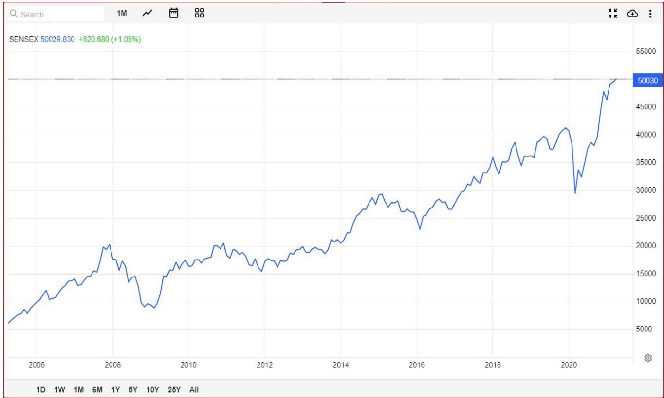Accordingly, the reference period of 13 years is divided as: $$ 2007-08\&2008-09\rightarrow\text{Recession/Bearish Phase} $$ $$ 2 0 0 9 - 1 0 \text{t o} 2 0 1 3 - 1 4 \rightarrow \text{RecoveryPhase} $$ $$ 2014-15 to 2019-20 \rightarrow Normal/Bullish Phase $$  Sensex Graph [2007-2020] ### c) Sampling The Universe for the present study is listed pharmaceutical companies in India. To ensure that a reasonable & true representative Sample is drawn for the study, sampling process used the following filters: 1. Only the Companies which have remained listed during the reference period, were selected. 2. Companies which were actively traded during the reference period have been selected 3. All the companies with complete required data available for the entire reference period were selected 4. Companies with Accounting period of 12 months coinciding with the financial Year for all the years under study were selected. The companies so drawn were arranged in an ascending order as per their TDTA ratio. $25\%$ of the companies, totalling 10 companies, at the top end of the order were selected as sample for the study. Thus, the sample constituted the highest debt companies of the pharmaceutical sector. ### d) Variables ## i. Independent Variables The independent variable for the study is financial leverage. Financial leverage refers to the magnification of risk and return introduced through the use of fixed-cost financing, such as debt and preferred stock. The more fixed-cost debt a firm use, the greater will be its expected risk and return. [L. J. Gitman]. Financial leverage has been Poxied by. Total Debt to Total Assets TD/TA Long Term Debt to Total Assets LTD/TA Short Term Debt to Total Assets STD/TA ## ii. Dependent Variables Since the study aims to assess the impact of financial leverage on firm performance specifically in terms of Shareholders payoffs, therefore, the dependent variables for the present study include Return on Equity (Hasson and Gupta, 2013), and Earning per share (Abar, 2005). #### 1. Return on Equity Return on equity reveals profitability of Owners' investment. Therefore, it indicates how well the company has used Owners' capital. The operational definition of ROE is. $$ \mathrm{ROE} \quad = \quad \frac{\mathrm{Net\,profit\,after\,Tax}}{\mathrm{Average\,Equity}} $$ ### 2. Earnings Per Share (EPS) It refers to net earnings per equity share. Earnings per shares are the portion of a company's profit that is allocated to every individual share of the stock. The operational definition of EPS for this study is: $$ \begin{array}{r l r} {\mathrm{E P S}} & = & \underline{{\text{NetEarningsavailableforEquity}}} \\& & \underline{{\text{Numberofoutst and ingEquityShares}}} \end{array} $$ ## iii. Control Variables In addition to financial leverage, there are other factors which are likely to have an impact on the profitability of a company, [Osuji Casmir (2012)]. Hence to assess the impact of financial leverage on payoffs to stockholders, other factors that are likely to have impact on profitability need to be controlled. It is in view of this fact, that some controlling variables have been added in the study which include tangibility, sales growth & growth opportunities. The operational definition of these control variables is given below:- $$ Tangibility of firm = \frac{fixed assets}{total assets} $$ Sales growth of firm= $\frac{\text{CurrentYearsales} - \text{PreviousYearSales}}{\text{PreviousYearSales}}$ $$ G r o w t h \quad \text{opportunitie} = \frac{\text{TotalAssetsofCurrentYear - TotalAssetsofthePreviousyear}}{\text{TotalAssetsofthePreviousyear}} $$ ## iv. Econometric Model and Penal Data Estimation The study consists of both cross sectional units and time series data. Cross sectional units comprising of 10 companies and Time series covers a period of 13 years, slotted into three phases of an economy, thus paving the way for Penal Data Modeling. "Penal Data Modeling is efficient in comparison to pure cross-sectional or time series as it produces more informative data, uses more Degree of Freedom and observe less Collinearity among the variables" [Yadav. M.P et al (2022)]. First Poolability test was employed to check whether the data is Poolable or not. Then testing of cross-sectional effect was done to decide an application of suitable Model for the Penal Data Regression. [Li M et al (2015)]. If data is poolable, pooled regression is applied otherwise Fixed or Random Effect Models are employed. The Fixed Effect Model Controls for all time - invariant differences between the individuals, so the estimated coefficients of the Fixed Effect Models are unbiased because of omitted time - invariant characteristics as observed by Yadav & Yadav (2021). It is presented as: $$ \gamma_{it} = \alpha_{it} + \beta\chi_{it} + \mu_{it} $$ Where i and t are Cross Sectional Units (Company) and Time Period respectively. $\gamma_{it}$ is dependent variable of Company i at time t $\chi_{it}$ Independent variable $\alpha$ is Fixed over time and remodelling itself in accordance with different cross section units. $\mu_{it}$ is the error term In the aforesaid equation, impact of time – invariant variable cannot be estimated under the Fixed Effect Model because of their Omission. In this Model there exists correlation between Independent variable and unobserved heterogeneity and is fixed and constant across different Cross - Sectional Units. When this assumption is not fulfilled, it paves the way for Random Effect Model [REM] as in REM unobserved Heterogeneity behaves in a random fashion and has no correlation with the independent variables as being treated statistically independent of Explanatory variables. Thus will calculate the impact of variables that are not changing with the time. The representative equation is as under: $$ \gamma_{it} = \alpha_{it} + \beta_{it} \chi_{it} + \mu_{it} $$ Here $\alpha$ is treated as Random Variable as $i$ merges with the Error Term and starts acting like Error Term, hence the name Random Effect. It will follow the properties of Error Term as it is not being incorporated in it. [Dr. Miklesh Yadav (2021)]. Accordingly, the Regression Equation of Penal Data Methodology for this study would be: $$ \begin{array}{l} E P S _ {i t} = \alpha_ {i} + \beta_ {1} T D T A _ {i t} + \beta_ {2} L T D T A _ {i t} + \beta_ {3} S T D T A _ {i t} + \beta_ {4} G r o w t h _ {i t} + \beta_ {5} T a n g _ {i t} + \beta_ {6} S g r o w t h _ {i t} + \mu_ {i t} \\R O E _ {i t} = \alpha_ {i} + \beta_ {1} T D T A _ {i t} + \beta_ {2} L T D T A _ {i t} + \beta_ {3} S T D T A _ {i t} + \beta_ {4} G r o w t h _ {i t} + \beta_ {5} T a n g _ {i t} + \beta_ {6} S g r o w t h _ {i t} + \mu_ {i t} \\\end{array} $$ Where TD/TA, LTD/TA, STD/TA, Growth, Tang, S growth, are Total debt to Total Assets, Long Term Debt to Total Assets, Short Term Debt to Total Assets, Growth opportunities, Tangibility, Sales growth, of the company (i) at time (t) respectively. ## v. Penal Data Estimation Models The study used static penal data estimation models viz. first difference method, ordinary least square method, fixed effect model & random effect model as per the model fitness for different data sets. While applying the different models, model fitness in respect of a particular dependent variable was tested using poolability & Hausman tests. Poolability test determines whether the data set is poolable or not. If the p-value of the test is more than 0.05, the data set is poolable and Ordinary Least Square Method is fit for the analysis of the data set, otherwise fixed or random effects model is applicable which is found out by Housman test. In case of Hausman Test when Null Hypothesis is rejected (p-value $< 0.05$ or $5\%$ ) level of significance, FEM is more suitable otherwise REM is preferable. ## IV. DATA ANALYSIS AND INTERPRETATION The main objective of a firm is maximization of shareholders' wealth which depends on the financial performance of a company which in turn depends upon the efficiency with which decision-making is made whether financial or non-financial. One of such decisions is the capital structure decision. Although there is a difference of opinion with regard to the impact of financing decision on the value of firm. Relevant school of thought is of the opinion that there exists an optimum debt-equity mix at which the cost of capital is minimum and the value of firm is maximum. Contrary to this, the scholars belonging to irrelevant school of thought argue that the value of firm is independent of financing decision. Empirical studies conducted on this subject matter have revealed mixed results. Given the inconclusiveness of the studies conducted so far on this crucial aspect of corporate financial decision-making, the present study has been conducted with the sole purpose to assess the impact of debt on the payoffs to shareholders of the sample companies. However, before presenting the results of the data analysis, the descriptive statistics of the data set has been presented and discussed. ### a) Description Statistics Description statistics of three data sets viz. Independent Variable, Financial leverage, Dependent Variables, namely return on equity (ROE) & earnings per share (EPS) and control variables namely Growth opportunities, Tangibility & Sales growth of firms has been displayed in table 1. The descriptive analysis reveals basic statistical features like, mean, minimum, maximum, standard deviation skewness & kurtosis of various Variables. Table 1: Descriptive Statistics of Variables of Study. <table><tr><td>Variable</td><td>Mean</td><td>Median</td><td>Minimum</td><td>Maximum</td><td>Std. Dev.</td><td>C. V.</td><td>Skewness</td><td>Ex. kurtosis</td><td>J. B Tests</td></tr><tr><td>EPS</td><td>4.5559</td><td>3.475</td><td>-33.92</td><td>30.84</td><td>10.895</td><td>2.3913</td><td>-0.12064</td><td>1.1166</td><td>0</td></tr><tr><td>ROE</td><td>5.8855</td><td>6.335</td><td>-41</td><td>35.24</td><td>14.451</td><td>2.4554</td><td>-0.92593</td><td>1.3003</td><td>0</td></tr><tr><td>TD_TA</td><td>0.66775</td><td>0.67682</td><td>0.21332</td><td>0.838</td><td>0.10043</td><td>0.15039</td><td>-1.3687</td><td>3.5454</td><td>0</td></tr><tr><td>STD_TA</td><td>0.20785</td><td>0.20382</td><td>0.031236</td><td>0.487</td><td>0.10645</td><td>0.51216</td><td>0.74749</td><td>0.11055</td><td>0</td></tr><tr><td>LTD_TA</td><td>0.44536</td><td>0.45727</td><td>0.12</td><td>0.688</td><td>0.14138</td><td>0.31744</td><td>-0.47294</td><td>0.58131</td><td>0</td></tr><tr><td>Growth_oppo</td><td>0.10442</td><td>0.090236</td><td>-0.2105</td><td>0.68</td><td>0.16551</td><td>1.5851</td><td>1.2651</td><td>2.5214</td><td>0</td></tr><tr><td>TANG</td><td>0.37448</td><td>0.3744</td><td>0.066</td><td>0.62904</td><td>0.11575</td><td>0.30909</td><td>-0.58827</td><td>0.69445</td><td>0</td></tr><tr><td>S_GROW</td><td>0.13828</td><td>0.1379</td><td>-0.41438</td><td>0.808</td><td>0.22227</td><td>1.6074</td><td>0.57995</td><td>0.92928</td><td>0</td></tr></table> From the data contained in the above table it can be observed that mean EPS of the companies depicts that companies have generated positive returns for shareowners in spite of wide variations in the Earnings per Share. Further, on an average, the returns to the Equity Shareholders' has been positive during the study period, regardless of wide variations. These wide variations in the dependent variables are due to different phases of an economy/market, which were witnessed during the reference period. Initial two years 2007-08 & 2008-09, the economy witnessed recession in the entire world including India. From 2009-10 to 2013-14, the economy/market witnessed recovery from the lows of recessionary phase. Post 2014 the Indian markets have registered some kind of bullish phase It can also be seen from the above table that both the dependent variables show negative skewness but positive kurtosis. The mean debt of the sample pharmaceutical companies during the reference period was $66.77\%$ of the total assets, which varied between a minimum of $21.33\%$ to a maximum of $83.8\%$ this implies that the debt levels of the sample pharmaceuticals companies during the reference period were neither more nor less. ### b) Assumption Testing #### 1. Normality test Normality of the data as revealed by the Skewness & Ex-kurtosis values, and further tested by J.B Test. The normality of the data set as shown by the table 1 is further refined by using the conventional cleaning procedure as recommended by Heir et al (2010). #### 2. Multicollinearity Test Multicollinearity refers to a situation in which two or more Predictory variables are highly correlated. It affects the interpretability of a Regression Model, since it comprises the essential significance of independent variables. To test the severity of Multicollinearity, Variance inflation factor [VIF] was used as: - $$ \begin{array}{l} \mathrm{V if} \sim 1 \rightarrow \text{negligibleCollinearity} \\V if > 1 \text{but} < 5 \text{moderateCollinearity} \\V if > 1 0. h i g h C o l l i n a r i t y \\\end{array} $$ This study has applied the rule of thumb, that is VIF more than 10 as extremely Collinear. From the table 2, it is evident that none of the variables shows Multicollinearity, as the VIF is less than 10 in case of all the Variables under study. Table 2: Diagnostic Tests of Variables of Study. <table><tr><td>Variable</td><td>Heteroscedasticity Test White&#x27;s Test (P-Value)</td><td>Autocorrelation Test (D-W Statistics)</td><td>Multicollinearity Test</td><td>Stationarity Test (VIF)</td></tr><tr><td>EPS</td><td>0.00209984</td><td>1.96793</td><td>1.898</td><td>0.0000</td></tr><tr><td>ROE</td><td>0.00237344</td><td>1.635973</td><td>2.093</td><td>0.0000</td></tr><tr><td>TDTA</td><td>2.05455e-05</td><td>1.99436</td><td>2.459</td><td>0.0000</td></tr><tr><td>STD/TA</td><td>0.310194042</td><td>1.79007</td><td>2.711</td><td>0.0000</td></tr><tr><td>LTD/TA</td><td>0.225127</td><td>1.8411</td><td>3.811</td><td>0.0203</td></tr><tr><td>G. Opp</td><td>0.18607</td><td>1.93883</td><td>1.239</td><td>0.0000</td></tr><tr><td>Tang</td><td>0.84821</td><td>1.837746</td><td>1.526</td><td>0.0023</td></tr><tr><td>Sales-Growth</td><td>0.444121</td><td>1.78927</td><td>1.245</td><td>0.0000</td></tr></table> #### 3. Heteroscedasticity Test Heteroscedasticity of the data is checked by white test [Eric Luse Kuto Mwambuli (2015)]. Null hypothesis of the test is Heteroscedasticity not present and alternative hypothesis is that data is heteroscedastic. Table 2 shows the presence of Heteroscedasticity in both EPS & ROE variables as the P-Value is significant for both of them. The heteroscedasticity is removed by taking the Robust Standard Error of these variables. #### 4. Autocorrelation Test Autocorrelation refers to the degree of correlation of the same variable between two successive time intervals. Durbin-Watson statistic is used to test the autocorrelation because of (i) its high power; and (ii) its limited size distortions. [Fisher (1935) and Pitman (1937)]. The outcome of D-W test ranges from 0 to 4 as: - - $0 \rightarrow$ stronger positive - $2 \rightarrow$ a very low level of autocorrelation - $4 \rightarrow$ stronger negative correlation Table 2 above shows that none of the variables suffer from strong Autocorrelation. ### c) Stationarity Test A series is said to be stationary when its mean and variance remain constant over a period of time or in other words its mean and variance are time independent. Regressing a non-stationary time series over another non-stationary time series will result in the spurious regression which will produce misleading results about the estimated parameters. Levin-Lin-Chu Test is used for testing stationarity of data which is being recommended for balanced panel data. The null hypothesis of the test is that the series has unit roots. As revealed by table 2, all the variables have P-Value less than 0.05, so null hypothesis is rejected. All the variables are thus stationary at I (0) Level. Since all the variables are Stationary at I (0) Level, thus in this scenario performing a cointegration test is not necessary. This is because any shock to the system in the short run quickly adjusts to the long-run. Consequently, only the long run model is to be estimated using OLS (where variables are neither lagged nor differenced). In essence, the estimation of short run model is not necessary if series are Stationary at I (0) Level. ## i. Correlation Analysis Correlation analysis is applied to assess the relationship among various variables using Karl Pearson's correlation matrix. The relationship between the dependent, independent and control variables is ascertained and the results so obtained have been presented in the table 3 Table 3: Correlation Matrix of Dependent, Independent & Control Variables. <table><tr><td>Variable</td><td>S_GROW</td><td>TANG</td><td>Growth_oppo</td><td>LTD_TA</td><td>STD_TA</td><td>TD_TA</td><td>ROE</td><td>EPS</td></tr><tr><td>EPS</td><td>0.1355</td><td>-0.0653</td><td>0.1109</td><td>-0.0881</td><td>-0.005</td><td>-0.0954</td><td>0.6538</td><td>1</td></tr><tr><td>ROE</td><td>0.3154</td><td>-0.136</td><td>0.1002</td><td>0.1478</td><td>-0.201</td><td>0.0257</td><td>1</td><td></td></tr><tr><td>TD_TA</td><td>-0.0225</td><td>-0.127</td><td>0.0234</td><td>0.557</td><td>0.0889</td><td>1</td><td></td><td></td></tr><tr><td>STD_TA</td><td>-0.1751</td><td>0.242</td><td>-0.02</td><td>-0.5926</td><td>1</td><td></td><td></td><td></td></tr><tr><td>LTD_TA</td><td>0.0457</td><td>-0.3083</td><td>-0.0096</td><td>1</td><td></td><td></td><td></td><td></td></tr><tr><td>Growth_oppo</td><td>0.2676</td><td>-0.3031</td><td>1</td><td></td><td></td><td></td><td></td><td></td></tr><tr><td>TANG</td><td>-0.0805</td><td>1</td><td></td><td></td><td></td><td></td><td></td><td></td></tr><tr><td>S_GROW</td><td>1</td><td></td><td></td><td></td><td></td><td></td><td></td><td></td></tr></table> From the above table, it is clear that EPS shows negative correlation with all the three Independent Variables, viz. TD/TA, STD/TA & LTD/TA while as ROE depicts positive correlation with TD/TA & LTD/TA but negative correlation with STD/TA. Evidently highest and positive correlation is observed between EPS & ROE. The data is further analysed by applying regression analysis using Gretl Software. The regression models used include, First Difference Method, Ordinary Least Square Method, Fixed Effect Model & Random Effect Model Prior to the application of regression analysis, the respective model fitness is ascertained by Poolobility and Housman Tests. ## ii. Test for Poolability Table 4: Poolability Test of Dependent Variables EPS & ROE. <table><tr><td>S. NO</td><td>VARIABLE</td><td>P-VALUE</td><td>POOLABLE/NOT POOLABLE</td><td>MODEL CONSISTENT</td></tr><tr><td>1</td><td>EPS</td><td>2.95973E-05</td><td>NOT POOLABLE</td><td>FIXED/RANDOM</td></tr><tr><td>2</td><td>ROE</td><td>0.000248718</td><td>NOT POOLABLE</td><td>FIXED/RANDOM</td></tr></table> Poolability of the data is checked by the test for differing group intercepts, the null hypothesis for which is, "The groups have common intercept" The p-values for EPS & ROE are both less than $5\%$, level of significance, so we reject the null hypothesis of common intercepts of groups and accept the alternate hypothesis that groups do not have common intercepts, which implies that the data set is not Poolable, therefore either Fixed or Random Effect Model is to be applied depending upon the results of Housman Test. ## iii. Housman Test To decide whether fixed of random model is consistent for the variable EPS & ROE, Housman test is applied. The results obtained are shown in table below. Table 5: Housman Test of Dependent Variables EPS & ROE. <table><tr><td>S. NO</td><td>VARIABLE</td><td>P-VALUE</td><td>MODEL CONSISTENT</td></tr><tr><td>1</td><td>EPS</td><td>0.000769613</td><td>FIXED EFFECT MODEL</td></tr><tr><td>2</td><td>ROE</td><td>1.89099e-06</td><td>FIXED EFFECT MODEL</td></tr></table> As revealed by table 5, P-value of both the variables is less than critical value [(5%) level of significance], thus the null hypothesis is rejected, implying that Fixed Effect Model is suitable for both the variables. Further analysis of the data is carried out in adherence to model consistency as disclosed by the table 5. Above. Table 6: Regression Coefficients of Dependent Variables EPS & ROE. <table><tr><td>DV</td><td></td><td>Regressors</td><td>coefficient</td><td>std. error</td><td>t-ratio</td><td>p-value</td></tr><tr><td rowspan="9">EPS</td><td></td><td>const</td><td>12.1514</td><td>5.32469</td><td>2.282</td><td>0.0484 **</td></tr><tr><td rowspan="3">IDV</td><td>TD_TA</td><td>-13.5272</td><td>5.54592</td><td>-2.439</td><td>0.0374 **</td></tr><tr><td>STD_TA</td><td>0.805281</td><td>9.67845</td><td>0.0832</td><td>0.9355</td></tr><tr><td>LTD_TA</td><td>3.82354</td><td>5.62469</td><td>0.6798</td><td>0.5137</td></tr><tr><td rowspan="3">Control variable</td><td>Growth_oppo</td><td>10.9545</td><td>5.97996</td><td>1.832</td><td>0.1002</td></tr><tr><td>TANG</td><td>-6.61112</td><td>9.7366</td><td>-0.6790</td><td>0.5142</td></tr><tr><td>S_GROW</td><td>6.50149</td><td>2.69949</td><td>2.408</td><td>0.0394 **</td></tr><tr><td colspan="2">LSDV R-squared 0.297835</td><td></td><td colspan="3">Within R-squared 0.074507</td></tr><tr><td colspan="2">Test statistic: F(6, 9) = 4.01467</td><td></td><td colspan="3">p-value = 0.0309302</td></tr><tr><td>DV</td><td></td><td>Regressors</td><td>coefficient</td><td>std. error</td><td>t-ratio</td><td>p-value</td></tr><tr><td rowspan="9">ROE</td><td></td><td>const</td><td>-0.623100</td><td>8.93991</td><td>-0.06970</td><td>0.946</td></tr><tr><td rowspan="3">IDV</td><td>TD_TA</td><td>-13.6951</td><td>14.1812</td><td>-0.9657</td><td>0.3594</td></tr><tr><td>STD_TA</td><td>-5.31107</td><td>8.0838</td><td>-0.6570</td><td>0.5276</td></tr><tr><td>LTD_TA</td><td>22.5067</td><td>18.3663</td><td>1.225</td><td>0.2515</td></tr><tr><td rowspan="3">Control variable</td><td>Growth_oppo</td><td>3.21275</td><td>8.95787</td><td>0.3587</td><td>0.7281</td></tr><tr><td>TANG</td><td>10.7022</td><td>23.2056</td><td>0.4612</td><td>0.6556</td></tr><tr><td>S_GROW</td><td>17.2874</td><td>4.45331</td><td>3.882</td><td>0.0037***</td></tr><tr><td colspan="2">LSDV R-squared 0.333865</td><td></td><td colspan="3">Within R-squared 0.120644</td></tr><tr><td colspan="2">Test statistic: F(6, 9) = 9.33721</td><td></td><td colspan="3">p-value = 0.00192033</td></tr></table> Form the table NO. 6, it is evident that EPS has negative and statistically significant relationship with TD/TA at $5\%$ level of significance. It means that with the increase in ratio of total debt to total assets, the returns to the shareholders decreases when measured in terms of EPS. In other words, it can be said that high debt content in the capital structure of the sample companies adversely effects the return to the stockholders in terms of lower EPS. However, both STD/TA & LTD/TA show positive but insignificant relationship with the EPS. The null hypothesis that the financial leverage has no impact on the shareholders payoffs is rejected in terms of EPS when measured in relation to total debt to total assets. The results are in line with Majumdar & Chhiber (1997); Roa M, Yahyaee & Syed (2007); Aatherine Njagi (2012) Sabar Akbarian 2013.Raheel Mumtaz etal (2013), but are contrary to Lasher (2003), Nawaz, Javid & Akhtar (2012), Mubeen & Akhtar (2014), Abdul Azeez et al (2015) etc. when the impact of financial leverage on EPS was assessed with relation to STD to TA & LTD to TA there was insufficient evidence to conclude that there is an impact of financial leverage. The model is significant as the p-value is 0.0309302 i.e. lower than the critical value. The above referred table also discloses that ROE has statistically insignificant inverse relationship with TD/TA & STD/TA but insignificant positive relation with LTD/TA. The negative relation of ROE with TD/TA is in contradiction with the correlation analysis results, as well as with the null hypothesis. The results of regression analysis of STD/TA & LTD/TA are in conformity with the correlation analysis results. LTDTA shows insignificant positive relationship with both the dependent variables viz. EPS & ROE, but STDTA depicts insignificant positive and negative relationship with EPS & ROE respectively. ### d) Periodical Analysis Since it was intended to ascertain the impact of financial leverage on the payoffs to the stockholders in different phases of economy/market, the study was accordingly carried out separately for each phase as well. The three phases were identified on the basis of economic/market conditions as depicted by the Sensex graph, deemed as the barometer of the economic conditions especially in relation with financial performance of corporate sector. The three phases are labelled as Recessionary/Bearish Phase, Recovery Phase and Normal/Bullish Phase of Economy/Market. Regression analysis of the data sets for these respective phases has been conducted and the results so obtained are presented in their respective tables as follows. ## i. Recession/Bearish Phase The recession/bearish market phase started with what is commonly called as, "Bursting of Housing Bubble" in 2007 and continued for two years, 2007-08 & 2008-09. It lasted for short period & the economy immediately started to recover from the shock which originated in the western nations and had global ramifications though with varying intensities in different countries, wherein some countries suffered more & some less. An attempt has been made to ascertain the impact of financial leverage on the sample pharmaceutical companies during this recessionary/bearish phase of the economy/market using regression analysis. First Difference Method of regressing is applied as the period of recession is only of two years. The regression results so obtained are presented in the table 7 below. Table 7: Regression Coefficients of Dependent Variables-EPS & ROE during Recessionary/Bearish Phase. <table><tr><td>DV</td><td></td><td>Regressors</td><td>coefficient</td><td>std. error</td><td>t-ratio</td><td>p-value</td></tr><tr><td rowspan="9">EPS</td><td></td><td>const</td><td>5.05921</td><td>5.79445</td><td>0.8731</td><td>0.4053</td></tr><tr><td rowspan="3">IDV</td><td>d_TD_TA</td><td>-26.5522</td><td>124.165</td><td>-0.2138</td><td>0.8354</td></tr><tr><td>d_STD_TA</td><td>-2.45082</td><td>64.7206</td><td>-0.03787</td><td>0.9706</td></tr><tr><td>d_LTD_TA</td><td>-17.8368</td><td>111.718</td><td>-0.1597</td><td>0.8767</td></tr><tr><td rowspan="3">Control variable</td><td>d_Growth_oppo</td><td>-23.2599</td><td>16.8034</td><td>-1.384</td><td>0.1996</td></tr><tr><td>d_TANG</td><td>-65.1102</td><td>37.9269</td><td>-1.717</td><td>0.1202</td></tr><tr><td>d_S_GROW</td><td>33.7581</td><td>16.1815</td><td>2.086</td><td>0.0666*</td></tr><tr><td>R-squared</td><td>0.627726</td><td rowspan="2"></td><td colspan="3">Adjusted R-squared -0.116823</td></tr><tr><td>F(6, 9)</td><td>2.511827</td><td>P-value(F)</td><td colspan="2">0.103590</td></tr><tr><td>DV</td><td></td><td>Regressors</td><td>coefficient</td><td>std. error</td><td>t-ratio</td><td>p-value</td></tr><tr><td rowspan="8">ROE</td><td></td><td>const</td><td>8.23088</td><td>6.93271</td><td>1.187</td><td>0.2655</td></tr><tr><td rowspan="3">IDV</td><td>d_TD_TA</td><td>-33.7705</td><td>145.532</td><td>-0.2320</td><td>0.8217</td></tr><tr><td>d_STD_TA</td><td>-3.01783</td><td>75.6404</td><td>-0.03990</td><td>0.969</td></tr><tr><td>d_LTD_TA</td><td>14.3459</td><td>131.746</td><td>0.1089</td><td>0.9157</td></tr><tr><td rowspan="3">Control variable</td><td>d_Growth_oppo</td><td>-6.97031</td><td>19.5279</td><td>-0.3569</td><td>0.7294</td></tr><tr><td>d_TANG</td><td>-17.9995</td><td>46.0195</td><td>-0.3911</td><td>0.7048</td></tr><tr><td>d_S_GROW</td><td>38.0606</td><td>21.2417</td><td>1.792</td><td>0.1068</td></tr><tr><td>R-squared</td><td>0.575167</td><td></td><td colspan="3">Adjusted R-squared -0.274499</td></tr></table> From table 7 it is evident that EPS has statistically insignificant negative relationship with all the three proxies of financial leverage, viz. TDTA, STDTA & LTDTA. While as, ROE shows positive relationship with LTDTA and negative relationship with other two proxies of financial leverage but the relationship is statistically insignificant in all the cases. This insignificant relationship is against the general belief that during the recessionary phase there is adverse effect of financial leverage on the financial performance of the companies and the effect is more severe in case of companies having high content of debt in their capital mix. This insignificant effect is probably because of the two fold reasons of short span of recessionary phase and the intensity of recession was low in India. The results reject our alternative hypothesis of an impact of financial leverage on the shareholders payoffs. ## V. RECOVERY PHASE As already stated that the recessionary phase lasted for two years (2007-08 & 2008-09) and the economy started recovering from the housing bubble shock from the year 2009-10. The recovery phase was spanned over five years till 2013-14. The impact of financial leverage on the performance of the sample companies during the recovery phase was assessed by using regression analysis. But before the application of regression analysis the regression model fit for the respective data set of the recovery phase was determined by Poolability test and Housman test. ### a) Poolability Test Poolability test is applied to find out whether the data is poolable or not. The null hypothesis of the test is that the groups have the common intercept. When the p-value of the test is more than the critical value i.e. 0.05 or $5\%$, the null hypothesis is accepted. That means the data is poolable and the Ordinary Least Method of regression is fit for the analysis of the data set. However, when the p-value of the test is less than the 0.05 or $5\%$, the null hypothesis is rejected implying thereby that the data is not poolable and Ordinary Least Squares Method is not fit for the regression of the data sets. Under such situation either the Fixed or Random Effect Model is fit. The fitness of the model between the two is determined by Housman test. Table 8: Poolibility Test of two Dependent Variables EPS & ROE Recovery Phase. <table><tr><td>S. NO.</td><td>VARIABLE</td><td>P-VALUE</td><td>POOLABLE/NOT POOLABLE</td><td>MODEL CONSISTENT</td></tr><tr><td>1</td><td>EPS</td><td>0.177101</td><td>POOLABLE</td><td>ODINARY LEAST SQUARE METHOD</td></tr><tr><td>2</td><td>ROE</td><td>0.301935</td><td>POOLABLE</td><td>ODINARY LEAST SQUARE METHOD</td></tr></table> Since the p-value of the tests for both the variables viz. EPS & ROE is more than the critical value 0.05 or $5\%$, so the data sets are poolable and Ordinary Least Square method of regression is fit to be applied for the regression of the data sets, the results drawn are shown in the table 8 below Table 9: Regression Coefficients of Dependent Variables EPS & ROE during the Recovery Phase. <table><tr><td>SDV</td><td></td><td>Regressors</td><td>coefficient</td><td>std. error</td><td>t-ratio</td><td>p-value</td></tr><tr><td rowspan="9">EPS</td><td></td><td>const</td><td>41.6138</td><td>31.2974</td><td>1.33</td><td>0.2164</td></tr><tr><td rowspan="3">IDV</td><td>TD_TA</td><td>-38.3515</td><td>43.3649</td><td>-0.8844</td><td>0.3995</td></tr><tr><td>STD_TA</td><td>-1.75220</td><td>20.6603</td><td>-0.08481</td><td>0.9343</td></tr><tr><td>LTD_TA</td><td>-2.64820</td><td>16.0325</td><td>-0.1652</td><td>0.8725</td></tr><tr><td rowspan="3">Control variable</td><td>Growth_oppo</td><td>-9.78180</td><td>11.3492</td><td>-0.8619</td><td>0.4111</td></tr><tr><td>TANG</td><td>-22.9643</td><td>12.1649</td><td>-1.888</td><td>0.0917*</td></tr><tr><td>S_GROW</td><td>10.3355</td><td>11.8937</td><td>0.869</td><td>0.4074</td></tr><tr><td>R-squared</td><td>0.121165</td><td rowspan="2"></td><td colspan="3">Adjusted R-squared -0.035463</td></tr><tr><td>F (6, 9)</td><td>2.333652</td><td>P-value (F)</td><td colspan="2">0.122048</td></tr><tr><td>DV</td><td></td><td>Regressors</td><td>coefficient</td><td>std. error</td><td>t-ratio</td><td>p-value</td></tr><tr><td rowspan="9">ROE</td><td></td><td>const</td><td>36.5908</td><td>31.1603</td><td>1.174</td><td>0.2704</td></tr><tr><td rowspan="3">IDV</td><td>TD_TA</td><td>6.07678</td><td>40.7978</td><td>0.1489</td><td>0.8849</td></tr><tr><td>STD_TA</td><td>-58.1315</td><td>23.9362</td><td>-2.429</td><td>0.0381**</td></tr><tr><td>LTD_TA</td><td>-27.8510</td><td>28.4884</td><td>-0.9776</td><td>0.353</td></tr><tr><td rowspan="3">Control variable</td><td>Growth_oppo</td><td>-11.0843</td><td>16.1276</td><td>-0.6873</td><td>0.5092</td></tr><tr><td>TANG</td><td>-28.5102</td><td>21.9039</td><td>-1.302</td><td>0.2254</td></tr><tr><td>S_GROW</td><td>19.9356</td><td>11.7126</td><td>1.702</td><td>0.1229</td></tr><tr><td>R-squared</td><td>0.228364</td><td rowspan="2"></td><td>Adjusted R-squared</td><td colspan="2">0.120694</td></tr><tr><td>F(6, 9)</td><td>9.699443</td><td>P-value (F)</td><td colspan="2">0.001670</td></tr></table> Like the recessionary phase, the relationship of EPS with all the three proxies of financial leverage during the recovery phase was also negative and statistically insignificant. However, other variable ROE shows statistically significant negative relationship with STDTA at $5\%$ level of significance, the p-value being 0.0381 but the other two proxies viz. TDTA & LTDTA show insignificant positive and negative relationship with ROE respectively. The significant negative relationship of ROE with STDTA indicates that increase in the short term debt component in the overall capital, decreases the return to the shareholders in terms of ROE. The average STD in the sample companies is about one third of the average total debt of the sample companies. ### b) Normal/Bullish Phase It took almost five years for the economy to reach to the pre-recession levels. As such the normal ## i. Poolability Test phase of the economy started from the year 2014-15 as is clear from the forgoing Sensex graph, when the graph touched the same height from where it had dipped. This good growth period continued till the world was hit by the Covid-19 pandemic, definitely for a very short period of time. Thereafter, it showed a steep hike. Generally, it is believed that during the times of normal/bullish phase of economy/market, the companies with high debt deliver good returns to their stockholders, particularly due to the effect of trading on equity. How for this general belief holds good in the case of sample pharmaceuticals companies was ascertained by applying suitable model of regression analysis determined by Poolability & Housman tests. Table 10: Poolability Test of Dependent Variables EPS & ROE during Normal/Bullish Phase. <table><tr><td>S. NO.</td><td>VARIABLE</td><td>P-VALUE</td><td>POOLABLE/NOT POOLABLE</td><td>MODEL CONSISTENT</td></tr><tr><td>1</td><td>EPS</td><td>0.000529089</td><td>NOT POOLABLE</td><td>FIXED/RANDOM</td></tr><tr><td>2</td><td>ROE</td><td>0.00137651</td><td>NOT POOLABLE</td><td>FIXED/RANDOM</td></tr></table> The poolability test of the data sets indicated that both the dependent variables viz. EPS & ROE are not poolable, since p-values of test for both the variables were less than the 0.05, the admit table level of significance, as such either Fixed or Random Effect Model was fit for the data sets for its result oriented analysis. The fitness of the model between the two regression models was detected by Housman test. ## ii. Housman Test Housman test is applied to determine the fitness of the regression model among the fixed and random effect models. The null hypothesis for the test is that the GLS estimates are consistent. The null hypothesis is accepted when the p-value of the test is greater than the critical value 0.05 (5%), otherwise rejected when the p-value of the test is less than 0.05(5%). The rejection of null hypothesis means that fixed effect model is fit for the data set and the acceptance of the null hypothesis means that the random effect model of regression analysis is fit for the analysis of the data set of the dependent variable as is case here. For both the dependent variables, EPS & ROE the p-values of the test are greater than the critical value (5%), so random effect model is fit for the regression analysis of the data sets. Table 11: Housman Test of Dependent Variables, EPS & ROE during Normal/Bullish Phase. <table><tr><td>S. NO.</td><td>VARIABLE</td><td>P-VALUE</td><td>MODEL CONSISTENT</td></tr><tr><td>1</td><td>EPS</td><td>0.909447</td><td>RANDOM EFFECT MODEL</td></tr><tr><td>2</td><td>ROE</td><td>0.963523</td><td>RANDOM EFFECT MODEL</td></tr></table> Thus the regression analysis of the two data sets of dependent variables EPS & ROE was carried out by the random effect model as indicated by Housman test and the results so obtained are presented in table 12 below Table 12: Regression Coefficients of Dependent Variables EPS & ROE during the Normal/Bullish Phase. <table><tr><td>DV</td><td></td><td>Regressors</td><td>coefficient</td><td>std. error</td><td>Z</td><td>p-value</td></tr><tr><td rowspan="9">EPS</td><td></td><td>const</td><td>-9.45807</td><td>10.0797</td><td>-0.9383</td><td>0.3481</td></tr><tr><td rowspan="3">IDV</td><td>TD_TA</td><td>-17.9187</td><td>13.3685</td><td>-1.340</td><td>0.1801</td></tr><tr><td>STD_TA</td><td>5.9589</td><td>20.4361</td><td>0.2916</td><td>0.7706</td></tr><tr><td>LTD_TA</td><td>33.9002</td><td>12.6964</td><td>2.67</td><td>0.0076***</td></tr><tr><td rowspan="3">Control variable</td><td>Growth_oppo</td><td>19.2654</td><td>11.1253</td><td>1.732</td><td>0.0833*</td></tr><tr><td>TANG</td><td>21.0956</td><td>15.2395</td><td>1.384</td><td>0.1663</td></tr><tr><td>S_GROW</td><td>0.775329</td><td>9.64396</td><td>0.0804</td><td>0.9359</td></tr><tr><td colspan="2">quasi-demeaning = 0.669324</td><td></td><td colspan="3">corr(y,yhat)^2 = 0.0617846</td></tr><tr><td colspan="2">Chi-square(6) = 44.5012</td><td></td><td colspan="3">with p-value = 5.87936e-08</td></tr><tr><td>DV</td><td></td><td>Regressors</td><td>coefficient</td><td>std. error</td><td>Z</td><td>p-value</td></tr><tr><td rowspan="9">ROE</td><td></td><td>const</td><td>-7.24960</td><td>12.3485</td><td>-0.5871</td><td>0.5571</td></tr><tr><td rowspan="3">IDV</td><td>TD_TA</td><td>-44.5305</td><td>16.1811</td><td>-2.752</td><td>0.0059***</td></tr><tr><td>STD_TA</td><td>43.2248</td><td>22.3991</td><td>1.93</td><td>0.0536*</td></tr><tr><td>LTD_TA</td><td>67.6218</td><td>23.5951</td><td>2.866</td><td>0.0042***</td></tr><tr><td rowspan="3">Control variable</td><td>Growth_oppo</td><td>9.28632</td><td>5.88559</td><td>1.578</td><td>0.1146</td></tr><tr><td>TANG</td><td>2.81806</td><td>21.115</td><td>0.1335</td><td>0.8938</td></tr><tr><td>S_GROW</td><td>16.5008</td><td>11.3921</td><td>1.448</td><td>0.1475</td></tr><tr><td colspan="2">quasi-demeaning = 0.659512</td><td></td><td colspan="3">corr(y,yhat)^2 = 0.0976242</td></tr><tr><td colspan="2">Chi-square(6) = 37.5236</td><td></td><td colspan="3">with p-value = 1.39185e-06</td></tr></table> From table 12 it is observed that TDTA has negative relationship with both the indicators of the financial performance (EPS & ROE) of the sample companies. However, this negative relationship of TDTA with EPS & ROE is statistically insignificant in case of EPS but significant with ROE at $1\%$ level of significance. Both the dependent variables viz. EPS & ROE show positive relationship with STDTA but insignificant with EPS and significant with ROE at $10\%$ (0.0536) level of significance. LTDTA which forms about two third of the mean TDTA shows positive relationship with both EPS & ROE and in both cases the relationship is statistically significant at $1\%$ level of significance as their respective p-values are 0.0076 & 0.0042. It implies that during the normal/bullish phase of economy/market, LTDTA has a favourable effect on the financial performance of the sample companies. In other words, it can be said that during the normal/bullish phase of economy/market, more long term debt in the capital mix of the company can be beneficial. However, at the same time it is observed that TDTA has negative relationship with both the indicators of financial performance viz. EPS & ROE, though insignificant with EPS but significant with ROE at $1\%$ (0.0059) level of significance. This situation leads us to infer that the debt content in the debt equity mix of a company is financially beneficial to it during the normal economic phase but only to a certain limit and higher amounts of debt content in the capital mix will have negative impact on the financial performance of the company during the normal phase of economy in the case of pharmaceutical sector, as is reflected by the negative relationship of TDTA with EPS & ROE. The ratio of the TDTA is more than LTDTA due to inclusion of STDTA in it along with LTDTA. As such it can be concluded that during the normal phase of economy/ market inclusion of limited debt content in the capital mix of a pharmaceutical company can be financially advantageous to its shareholders in terms of EPS & ROE. The findings are in line with the Trade-off Theory of the Capital Structure which advocates for striking of trade-off between the costs and benefits of debt finance, so as to have the minimum weighted average cost of capital and maximum returns to its shareholders. ## VI. RESULTS, DISCUSSIONS AND CONCLUSIONS Generally, companies use both sources of Funds in their capital structure in different proportions which vary from country to country and within the country, industry to industry and even company to company within an industry. The Pharmaceutical Companies in India have used both the sources of funds in their Capital Structure. Whether the debt fund as used by the Pharmaceutical Companies magnify the shareholders' wealth or not was the subject matter of this research work. Accordingly, the researcher undertook a detailed & systematic analysis of the relevant data, the results of which are presented in the forgoing Chapters. From the forgoing results of multilinear regression analysis, it is evident that the financial leverage adversely effects the financial performance of the sample pharmaceutical companies in terms of EPS. While as in terms of ROE, the insignificant adverse relationship provided insufficient evidence to conclude that there is an impact of financial leverage on the financial performance of the sample companies. Therefore, the study reveals inconclusive results with regard to the impact of financial leverage on the financial performance when measured in terms of ROE & EPS which are the two sides of the same. The analytical results of the recessionary phase revealed an insignificant relationship of financial leverage with the firm performance. The results did not support the general belief of the corporate world that during recession phase of economy, the companies suffer financially and high debt companies suffer more. It is probably due to two fold reasons of very short span of recessionary phase coupled with the low intensity as was felt in India. Likewise, the mixed insignificant positive and negative results of regression analysis of the data sets of recovery period do not provide sufficient evidence regarding the impact of financial leverage on the financial performance of the sample pharmaceuticals companies. Only STDTA showed significant negative relationship with ROE at $5\%$ level of significance. The reason for the same may be that that STDTA forms around one third of the total debt. Theoretically, it is a general perception in the corporate world that during normal/bullish phase of the economy/market, the companies will dispense better financial performance to its shareholders particularly due to trading on equity. However, this theoretical perception is partially supported by the empirical findings as both negative and positive impact of financial leverage was observed during the normal/bullish phase. While TDTA showed significant negative impact of financial leverage on the firm performance in terms of ROE at $1\%$ level of significance, the LTDTA revealed significant positive relationship with both the indicators of firm performance viz. EPS & ROE that too at $1\%$ level of significance. This negative and positive relationship of proxies of financial leverage with the two indicators of firm performance leads to infer that the debt content, up to a certain level, in the debt-equity mix can magnify the financial returns of the sample pharmaceutical companies, but beyond that level of financial leverage the sample pharmaceuticals will suffer financially. The results are in line with the Trade-off Theory of Capital Structure which propounds for striking a trade-off between the costs and benefits of debt financing so as to have the optimal capital structure. At the same time, the findings negate the irrelevance school of thought. Further the findings are similar to the empirical findings of Abolaji Daniel et al (2020), who found a positive impact of financial leverage in the listed pharmaceuticals companies of Nigeria but are contrary to the empirical findings of BadriaMunthashofi et al. (2018), who reported negative impact of financial leverage on the profitability of listed pharmaceutical companies of Indonesia. a) Future Research Prospectus 1. Inclusion of unlisted Companies 2. Longer time periods. 3. Selection of companies at same (almost same) stage of growth. 4. Inclusion of more and more control variable for better results. 5. Alternate measures of Proxies to be used.

Generating HTML Viewer...

References

83 Cites in Article
Anifowose Abolaji,Soyebo,& Yusuf,Tanimojo Temitope (2020). Effect of Financial Leverage on Firms Performance: Case of Listed Pharmaceutical Firms in Nigeria.
Joshua Abor,N Biekpe (2005). The effect of capital structure on profitability: an empirical analysis of listed firms in Ghana.
N Abu-Rub (2012). Capital structure and firm performance: Evidence from Palestine stock exchange.
Sadia Afroze,Ahmed Khan,Shawrin (2022). Impact of Capital Structure on Firm Performance: Evidence from the Pharmaceuticals & Chemicals Sector in Bangladesh.
R Aggarwal,X Zhao (2007). The leverage-value relationship puzzle: An industry effects resolution.
Khalaf Al-Taani (2013). The Relationship between Capital Structure and Firm Performance: Evidence from Jordan.
Fred Arditti (1967). RISK AND THE REQUIRED RETURN ON EQUITY.
Ramachandran Azhagaiah,Candasamy Gavoury (2011). INTERRELATIONSHIP BETWEEN EQUITY-DEBT STRUCTURE AND PROFITABILITY WITH SPECIAL REFERENCE TO TEXTILE INDUSTRY IN INDIA.
D Baron (1974). Default risk, homemade leverage, and the Modigliani-Miller theorem.
Allen Berger,Emilia Bonaccorsi Di Patti (2006). Capital structure and firm performance: A new approach to testing agency theory and an application to the banking industry.
Laxmi Bhandari (1988). Debt/Equity Ratio and Expected Common Stock Returns: Empirical Evidence.
J Bitok,L Kibet,J Tenai,M (2011). The Determinants of Leverage at the Nairobi Stock Exchange, Kenya.
Laurence Booth,Varouj Aivazian,Asli Demirguc‐kunt,Vojislav Maksimovic (2001). Capital Structures in Developing Countries.
Saurabh Chadha,Anil Sharma (2015). Capital Structure and Firm Performance: Empirical Evidence from India.
D Champion (1999). Finance: the joy of leverage.
Lecheng Chen (2023). Impact of Capital Structure on the Operating Performance of Listed Companies in the Pharmaceutical Industry.
F Dare,S Olorunfemi (2010). Capital structure and corporate performance in Nigeria petroleum industry: Panel data analysis.
R Deesomsak,K Paudyal,G Pescetto (2004). the determinants of capital structure: Evidence from the Asia Pacific region.
J De Wet (2006). Determining the optimal capital structure: a practical contemporary approach.
Harry Deangelo,Ronald Masulis (1980). Optimal capital structure under corporate and personal taxation.
Valentin Dimitrov,Prem Jain (2008). The Value-Relevance of Changes in Financial Leverage Beyond Growth in Assets and GAAP Earnings.
Hung Dinh,Cuong Pham (2020). The Effect of Capital Structure on Financial Performance of Vietnamese Listing Pharmaceutical Enterprises.
D Durand (1952). Cost of debt and equity funds for business: Trends and problems of measurement.
I El-Sayed Ebaid (2009). The impact of capital-structure choice on firm performance: empirical evidence from Egypt.
Y Eunju,J Soocheong (2005). The effect of financial leverage on financial performance and risk of restaurant firms.
E Fama,K French (2010). Testing tradeoff and pecking order predictions about dividends and debt.
Murray Frank,Vidhan Goyal (2009). Capital Structure Decisions: Which Factors Are Reliably Important?.
A Ghosh,P Jain (2000). Financial leverage changes associated with corporate mergers.
L Gitman (2009). Principle of Managerial Finance.
K Gleason,L Mathur,I Mathur (2000). The interrelationship between culture, capital structure, and performance: evidence from European retailers.
Charles Hadlock,Christopher James (2002). Do Banks Provide Financial Slack?.
R Hamada (1972). The effect of the firm's capital structure on the systematic risk of common stocks.
A Handoo,K Sharma (2014). A study on determinants of capital structure in India.
A Hassan,A Gupta (2013). The effect of leverage on shareholders' return: An empirical study on some selected listed companies in Bangladesh.
Robert Haugen,Lemma Senbet (1978). THE INSIGNIFICANCE OF BANKRUPTCY COSTS TO THE THEORY OF OPTIMAL CAPITAL STRUCTURE.
P Hecht (2001). The cross section of expected firm (not equity) returns.
Armen Hovakimian,Tim Opler,Sheridan Titman (2001). The Debt-Equity Choice.
Tom Jacob,V Ajina (2020). Capital Structure and Financial Performance of Pharmaceutical Companies in Indian Stock Exchange.
B Javed,S Akhtar (2012). Interrelationships between Capital Structure and Financial Performance, Firm Size and Growth: Comparison of industrial sector in KSE.
A Kale (2014). The impact of financial leverage on firm performance: the case of non financial firms in Kenya.
E Kim (1978). A Mean-Variance Analysis of Optimal Capital Structures.
Michael King,Eric Santor (2008). Family values: Ownership structure, performance and capital structure of Canadian firms.
V Krishnan,R Moyer (1997). Performance, capital structure and home country: An analysis of Asian corporations.
M Kumar (2014). An Empirical Study on Relationship between Leverage and Profitability in Bata India Limited.
L Larry,R Ofek,Stulz (1995). Leverage investment and firm growth.
W Lasher (2016). Gale Cengage Learning.
J Lintner (1956). Distribution of incomes of corporations among dividends, retained earnings, and taxes.
S Majumdar,P Chhibber (1999). Capital structure and performance: Evidence from a transition economy on an aspect of corporate governance.
P Marsh (1982). The choice between equity and debt: An empirical study.
Neeti Mathur,Satish Tiwari,T Sita Ramaiah,Himanshu Mathur (2021). Capital structure, competitive intensity and firm performance: an analysis of Indian pharmaceutical companies.
John Mcconnell,Henri Servaes (1995). Equity ownership and the two faces of debt.
F Modigliani,M Miller (1958). The cost of capital, corporate finance and the theory of investments.
F Modigliani,M Miller (1963). Corporate income taxes and the cost of capital: A correction.
I Moosa,L Li (2012). Firm-specific factors as determinants of capital structure: evidence from Indonesia.
W Morton (1954). The Structure of the Capital Market and the Price of Money.
Mubeen Mujahid,Kalsoom Akhtar (2014). Impact of Capital Structure on Firms Financial Performance and Shareholders Wealth: Textile Sector of Pakistan.
B Munthashofi (2018). Financial Leverage and Profitability of Pharmaceutical Companies in Indonesia Stock Exchange.
Erick Mwambuli (2015). What Determines Corporate Capital Structure in Developing Economies? Evidence from East African Stock Markets.
L Mwangi,M Makau,G Kosimbei (2014). Relationship between capital structure and performance of non-financial companies listed in the Nairobi Securities Exchange, Kenya.
Stewart Myers,Nicholas Majluf (1984). Corporate financing and investment decisions when firms have information that investors do not have.
C Njagi (2013). The relationship between capital structure and financial performance of agricultural firms listed at Nairobi Securities Exchange.
O Oke,B Afolabi (2011). Capital Structure Composition and Financial Performance of Food and Beverage Firms in Nigeria.
C Osuji,A Odita (2012). Impact of capital structure on the financial performance of Nigerian firms.
A Ozkan (2001). Determinants of capital structure and adjustment to long run target: evidence from UK company panel data.
Krishna Pandey,Tarak Sahu (2019). Debt Financing, Agency Cost and Firm Performance: Evidence from India.
P Prakash,A Sindhasha (2016). A study on impact of leverage on profitability: Empirical evidence from select pharmaceutical companies in India.
Raluca-Georgiana Moscu (2014). Capital Structure and Corporate Performance of Romanian Listed Companies.
N Rao,K Al-Yahyaee,L Syed (2007). Capital structure and financial performance: evidence from Oman.
K Rayan (2010). Financial leverage and firm value.
M Sekar,Ms. Gowri,Ms. Ramya (2014). A Study on Capital Structure and Leverage of Tata Motors Limited: Its Role and Future Prospects.
Rakesh Sharma (2018). Factors affecting financial leveraging for BSE listed real estate development companies in India.
Atul Sheel (1994). Determinants of Capital Structure Choice and Empirics on Leverage Behavior: a Comparative Analysis of Hotel and Manufacturing Firms.
E Soloman (1963). The Theory of Financial Management.
Alpa Joshi (2013). A Study Of Profitability Analysis Of Selected FMCG Companies In India.
J Stiglitz (1969). A re-examination of the Modigliani-Miller theorem.
J Stiglitz (1974). Incentives and risk sharing in sharecropping.
R Stulz (1990). Managerial discretion and optimal financing policies.
R Taggart (1977). A Model of Corporate Financing Decisions.
S Titman,R Wessels (1988). The determinants of capital structure choice.
Arun Upneja,Michael Dalbor (2001). An examination of capital structure in the restaurant industry.
J Varghese,S Sahai (2021). Impact of Capital Structure on the Financial Performance of Firms: A Study of BSE Listed Selected Pharmaceutical Companies.
J Wald (1999). How firm characteristics affect capital structure: an international comparison.
Chenxin Zhang (2022). Impacts of Change in Capital Structure on the Profitability of Pharmaceutical Firms: A Study of Pharmaceutical Industry in Singapore.
No ethics committee approval was required for this article type.
Data Availability
Not applicable for this article.
How to Cite This Article
Bashir Amad Khan. 2026. \u201cExamining the Relationship Between Financial Leverage and Shareholder Payoffs: Insights from the Pharmaceutical Sector in India\u201d. Global Journal of Management and Business Research - C: Finance GJMBR-C Volume 23 (GJMBR Volume 23 Issue C4).
Explore published articles in an immersive Augmented Reality environment. Our platform converts research papers into interactive 3D books, allowing readers to view and interact with content using AR and VR compatible devices.
Your published article is automatically converted into a realistic 3D book. Flip through pages and read research papers in a more engaging and interactive format.
Our website is actively being updated, and changes may occur frequently. Please clear your browser cache if needed. For feedback or error reporting, please email [email protected]
Thank you for connecting with us. We will respond to you shortly.