Galactic space is filled with interstellar clouds of neutral gases. Motion of the spaceclouds is viewed as a flow of continuous fluid in curved space with gravity. Dynamical motions of the space-fluid of rotating galaxies are investigated by extending Fluid Dynamics to that in the frame of general relativity. Fluid flow field to be extended to that of a relativistic theory is reinforced by the fluid gauge theory equipped with a background (dark) gauge field conditioning the fluid continuity. The Gravity-space Fluid Dynamics thus developed captures main feature of the dark-matter effect as the action of the gauge field on the motion of space fluids. In the present formulation, the stress-energy tensor in the general relativity is revised in order to take account of general nature of stress field by extending the isotropic pressure to an-isotropic stress field.
## I. INTRODUCTION
The cosmological issue of dark matter effect is studied with a new approach to spiral galaxies in rotational motion (Fig.1). To that end, it is essential to recognize that, in cosmic space, gas clouds are abundant and free to move under physical fields: gravity field etc.
### a) Motion of space clouds viewed as continuous flows
The emission lines (such as the $HI - 21$ cm line) in cosmic space show abundance of neutral gas clouds in the galactic interstellar space. The neutral gases are captured by the galactic disk via its gravitational field and its spiral arms. Kalberla & Kerp (2009) coined it as Galactic Atmosphere over the galactic disk. Concerning the gas clouds moving about cosmic space, their dynamical motions should be described as flows of continuous fluids. Present study is carried out from this view on the basis of the Fluid Gauge Theory (Kambe 2021a).[^1]
Although stars are very sparse in outer part (halo) of our galaxy, the halo is dominated by invisible matters and actually contains considerable portion of the total mass of the galaxy. Present approach is based on the view that the dark matter effect might be caused by invisible space-fluids, driven by the action of a fluid gauge-field according to the theory. The space-fluids are moving at very-high orbital speeds of about $200\sim 300$ $\mathrm{km}\cdot \mathrm{s}^{-1}$ in the galactic space (Tully & Fisher (1977), Sofue & Rubin (2001), McGaugh et al. (2016)) under interaction with the galactic arms that rotate at high speeds as well. Dynamical mechanism of the interaction of space-fluids with the galactic arms moving at high orbital speeds is the target of the present investigation.
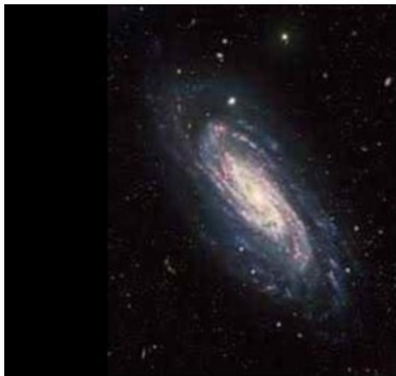 Figure 1: A sample spiral galaxy in rotation: NGC 3198 (GALEX image, NASA).
It is known that observed rotation curves of galaxies do not match the one expected from the Keplerian law of velocity decreasing as $R^{-1/2}$ with $R$ the distance from the gravity center. At distances away from the center, the stellar orbital motion tends to rotation with almost constant velocity. This hints that certain mechanism is working at halo parts of galaxies more conspicuously.
### b) Field description strengthened for rotational one
Present approach takes a new two-sided strategy, namely on the one hand the theory is strengthened by an improved action term of new stress field, on the other hand the dark object might be space-fluids existing abundantly in cosmic space. In fact, its flow field is reinforced by the fluid gauge theory equipped with a background (dark) gauge field (Kambe 2021a).
According to the theory, the isotropic pressure of Eulerian system is extended to an-isotropic stress fields giving rise to flows of rotational nature inherently. Thus, a new approach is formulated on the basis of the variation principle for a perfect fluid in the presence of gravity.
The present theory reinforces the fluid flow fields with a background (dark) gauge field. The gauge field not only ensures the mass conservation of fluid flows, but also assists the flow field with transition of its stress field $\sigma_{jk}$, from the isotropic pressure stress $p\delta_{jk}$ prevailing in quiet states of slow motion to an-isotropic stress field $M_{jk}$ prevailing in turbulent flow states.
In this regard, a past study of acoustics (Kambe 2022) is helpful to understand the transition. In the resonance problem studied by Kundt, increasing the strength of acoustic excitation triggers spontaneous transition of the acoustic field from isotropic to an-isotropic stress field. The an-isotropic rotational field is generated by an in visible gauge field and responsible to formation of the mysterious dust striations studied by Kundt (1866).
### c) Fluid Lorentz force
An important feature of the present theory is that it includes a new dark gauge-field $a_{\nu}$ ( $\nu = 0,1,2,3:$ relativistic 4-components). Incorporation of a non-gravitational field $a_{\nu}$ to the gravity field is assured by the local-flatness theorem (Schutz 1985) and the Einstein Equivalence Principle (Will 1993) in the general relativity. In addition to the gravitational Lagrangian built of metric alone yielding curved gravity space, fluid motions are described by new fluid Lagrangians. Thus new terms are introduced in equations of motion. The new terms are analogous to electromagnetic terms, but derived for neutral fluids here. One particular term to be remarked is the fluid Lorentz force, $\pmb{v} \times \pmb{b}$ with $\pmb{v}$ the fluid velocity and $\pmb{b}$ the fluid-magnetic field from $a_{\nu}$.
### d) Twisted connection between physics of galaxy rotation and visible matters
Physics of galaxy rotation is, in general, closely tied to the gravity field of baryonic visible matters. But in the present case, astronomical observations state that mutual relation between them is not straightforward.
Observing celestial objects within a spiral galaxy, their orbital velocities are detected spectroscopically at their respective distances from the galactic center, while the gravitational force is estimated from the data of baryonic visible mass distribution of stars and gases in the galaxy. The gravity forces thus obtained are not sufficient to reproduce the observed velocity curves at outer parts of most galaxies. This raised issues concerning presence of dark matters in most galaxies.
On the other hand, the recent study (McGaugh et al. 2016) proposed a universal behavior, stating that the rotational motion of a disk galaxy is determined entirely by visible matters it contains, even if the disk is filled with unknown dark matters, paradoxically. The last implies a strong twisted connection between the visible matters and the physics producing the rotational motion. Possible interpretations given by the authors of McGaugh et al. (2016) are rephrased in the following ways: either (a) it represents the end product of galaxy formation, or (b) it is the result of new dynamical laws rather than dark matter, or (c) it represents new physics of a dark sector that leads to the observed coupling.
Present study takes new double-sided approach both dynamically and physically: namely incorporating a new dynamical field of dark gauge-field and attacking the system with a new physics using an-isotropic stress fields. Therefore, present approach is related to both categories $(b)$ and $(c)$, in addition, with implicitly tak ing the view $(a)$. The present approach is based on the general-relativistic version of Fluid Gauge Theory.
### e) HI-21 cm line tells a mystery from cosmic space
Few galaxies exhibit the Keplerian law $v_{*} \propto R^{-1/2}$ for the stellar velocity $v_{*}$ at large distance $R$ from the galactic center, but the galactic rotation velocities keep high values at large values of $R$, flat instead of falling. This was recognized as early as 1950s (Sofue & Rubin 2001), and later updated to the Tully-Fischer relation (Tully & Fisher 1977): $M_{bar} \propto (v_{H})^{p}$ with $p = 3.5 \sim 4$, for the Hydrogen gas velocity $v_{H}$ at outer halo part of a galaxy and the total baryonic mass $M_{bar}$ of the galaxy, even in case with substantial dark matter. The Tully-Fisher relation does not show any variation with scale or size of galaxy, remarked by McGaugh (2005).
# f) A key
An important mathematical facet has been found for the galaxy dynamics by McGaugh et al. (2016), from statistics of a large set of 153 galaxies with different morphology, masses, sizes and gas fractions. Concerning the radial accelerations $A_{c}$ (toward the center) of orbiting celestial objects of rotating galaxies, the law says how the centripetal acceleration $A_{c}$ is related to the absolute value of gravity acceleration $A_{g}$.
To get an idea from simple analyses, let us take an axi-symmetric cylindrical coordinate system $(Z,R,\phi)$ with an axi-symmetric disk plane, defined by $Z = 0$. Consider a typical galaxy rotating around its center $(R = 0,Z = 0)$ with the velocity $(0,0,V(R))$, keeping steady state circular rotation.
In this circumstance, the observed centripetal acceleration is given by $A_{c} = V^{2}(R) / R$. On the other hand, from observed mass density distribution $\rho (R)$ within a galaxy, the gravity potential $\Phi_g$ is determined by solving $\nabla^2\Phi_g = 4\pi G\rho$, and the gravity acceleration $A_{g}$ is given by $A_{g} = |\partial \Phi_{g} / \partial R|$ ( $>0$, for clarity). A fitting curve was found by McGaugh et al. (2016) statistically, as
$$
A _ {c} = \mathcal {F} (A _ {g}) \equiv \frac {A _ {g}}{1 - e ^ {- \sqrt {A _ {g} / A _ {\dagger}}}}, \tag {1}
$$
where $A_{\dagger} \approx 1.20 \times 10^{-10} \, \mathrm{ms}^{-2}$. This implies a strong connection between the baryonic gravity acceleration $A_{g}$ and the physics that generates the observed $A_{c}$.
Looking at lower end of $A_{g}$ value (at halo part), the curve is found to be consistent with the Tully-Fischer relation. In fact, assuming $|A_{g} / A_{\dagger}| \ll 1$ and using $A_{c} \equiv (v_{H})^{2} / R$ and $A_{g} \propto M_{bar} / R^{2}$ as $R^{-1} \to 0$, the fitting curve (1) implies $M_{bar} \propto (v_{H})^{4}$, consistent with the Tully-Fischer relation.
The difference between $A_{c}$ and $A_{g}$ (if any) is accounted for as the contribution $A_{DM}$ from dark matter (DM): $A_{DM} = A_{c} - A_{g}$. However, the centripetal acceleration $A_{c}$ is given by the fitting function $\mathcal{F}(A_g)$. Thus, the $A_{DM}$ should be given by $\mathcal{F}(A_g) - A_g$, which is determined once $A_{g}$ is known regardless of DM. This means that the acceleration $A_{DM}$ (attributed to the dark matter) is coupled to the visible mass $\rho$ giving the gravitational acceleration $A_{g}$. Then where exactly is the freedom to be attributed to dark matter?
Regarding the sample galaxy NGC3198 (Fig.1), let us try to estimate magnitudes of $A_{c}$ and $A_{g}$ from available astronomical data (Venkataramani & Newell 2021). Its rotation curve shows: $V \approx 150\mathrm{km}\cdot \mathrm{s}^{-1}$ at $R \approx 19\mathrm{kpc}$ from the galactic center, which implies $A_{c}^{*} = V^{2} / R \approx 4.0 \times 10^{-11}\mathrm{ms}^{-2}$. Then the fitting curve (1) gives $A_{g}^{*} \approx 1.0 \times 10^{-11}\mathrm{ms}^{-2}$. From these two values, the DM contribution is estimated by the difference:
$$
A_{DM}^{*} = A_{c}^{*} - A_{g}^{*} \approx 3.0 \times 10^{-11} \mathrm{ms}^{-2}.
$$
One can remark a merit of their analysis. They are using acceleration terms, $A_{c}$, $A_{g}$ and $A_{DM}$. Hence, their arguments apply to any celestial object in accelerating motion without regard to its magnitude of mass: a star, a gas cloud, or a fluid particle of space-fluid.
### g) Invisible field creating visible effect
As one of the possible theories to resolve the current issue, the present paper proposes the Fluid Gauge Theory by extending the theory of fluid mechanics in flat space to the general relativity theory in curved space with gravity. The theory reinforces the fluid flow fields with a background (dark) gauge field. The new field strengthens the theory with two ways. The gauge field not only ensures the mass conservation of fluid flows, but also assists the flow field with transition of its stress field $\sigma_{jk}$, from the isotropic pressure $p\delta_{jk}$ prevailing in quiet states of slow motion to anisotropic stress field $M_{jk}$ prevailing in turbulent flows. This enables appropriate description for turbulent motions in cosmic space.
It is helpful to remember the case of Kundt-tube experiment (§1.2) to get insight into the present issue. It implies, "The gauge field within the Kundt-tube is not visible, yet creates visible dust-striations mechanically". This insight applies analogously to the gravitational potential $\Phi_g$ as well: The gravitational potential $\Phi_g$ is not visible, yet its derivatives $\partial_{\nu}\Phi_{g}$ create visible dynamical effect.
### h) Composition of the paper
Next section 2 describes the basic fluid system in flat space before extending to the general relativity in curved space. The fluid system is reinforced here by the fluid gauge theory equipped with a background (dark) gauge field. Extension to relativistic formulation according to the general relativity for curved space under gravity is carried out in the section 3 for isotropic pressure field where the stress-energy tensor of fluid motion is derived newly from the fluid Lagrangians. The section 4 explores what the part of the gauge field Lagrangians bring forward, and derives the equation of fluid motion under the anisotropic stress field. The dark matter effect of rotating spiral galaxies is investigated in section 5. Last section 6 summarises the outcomes of the present study. $^{1}$
## II. FLUID SYSTEM IN FLAT SPACE BEFORE EXTENDING TO CURVED SPACE
Relativistic formulation of Fluid Gauge Theory (FGT) is presented in Kambe (2021a) in flat space, which reinforces representation of the stress field within flows by adding rotational nature such as turbulence. This was achieved by extending the isotropic pressure field of Eulerian system to general anisotropic stress fields, according to the general gauge principle (Utiyama 1956).
### a) Lagrangians
According to the relativistic FGT theory (Kambe 2021a) in flat Lorentzian space, the fluid system is described by the total Lagrangian $\mathcal{L}^{\mathrm{FGT}}$ consisting of three components, $\mathcal{L}^{\mathrm{FGT}} = \mathcal{L}_{\mathrm{FM}} + \mathcal{L}_{\mathrm{int}} + \mathcal{L}_{\mathrm{GF}}$:
$$
\mathcal {L} _ {\mathrm {F M}} = - c ^ {- 1} \left(c ^ {2} + \bar {\epsilon} (\bar {\rho})\right) \bar {\rho}, \tag {3}
$$
$$
\mathcal {L} _ {\mathrm {i n t}} = c ^ {- 1} j ^ {\nu} a _ {\nu}, \tag {4}
$$
$$
\mathcal {L} _ {\mathrm {G F}} = - \left(4 \mu c\right) ^ {- 1} f ^ {\nu \lambda} f _ {\nu \lambda}, \tag {5}
$$
$$
f_{\nu\lambda} = \partial_{\nu} a_{\lambda} - \partial_{\lambda} a_{\nu},\quad \bar{\rho} \equiv \rho \sqrt{1 - \beta^2},
$$
where the overlined values denote proper values and $\beta = |\pmb{v}| / c$ (see Appendix A.ii) and the Lagrangian $\mathcal{L}_{\mathrm{GF}}$ includes a free parameter $\mu$ to be fixed later. The first Lagrangian $\mathcal{L}_{\mathrm{FM}}$ describes a perfect fluid in motion with 4-current mass flux $j^{\nu} = \rho v^{\nu}$ defined by (A2), and the third $\mathcal{L}_{\mathrm{GF}}$ describes an action of a background gauge field $a_{\nu}$ so as to ensure the fluid motion to satisfy mass conservation (to be shown later), while the middle $\mathcal{L}_{\mathrm{int}}$ describes their mutual interaction between $j^{\nu}$ and the gauge-field $a_{\nu}$.
Total action of this system $S^{\mathrm{FGT}}$ is defined by
$$
S^\mathrm{FGT} \equiv \int \mathcal{L}^{\mathrm{FGT}} \mathrm{d}\Omega = \int \left[ \mathcal{L}_{\mathrm{FM}} + \mathcal{L}_{\mathrm{int}} + \mathcal{L}_{\mathrm{GF}} \right] \mathrm{d}\Omega , \tag{7}
$$
where $\mathrm{d}\varOmega\equiv\mathrm{d}^4x^\nu=c\mathrm{d}t\mathrm{d}^3x$. It is helpful to consider the form of first term $\mathcal{L}_{\mathrm{FM}}$ under non-relativistic limit as $\beta \rightarrow 0$. The expression of $\mathcal{L}_{\mathrm{FM}}c\mathrm{d}^3x$ per unit mass $(m_{1}\equiv \rho \mathrm{d}^{3}x = 1)$ reduces to the non-relativistic form of $L_{nr}\equiv \frac{1}{2} m_1v^2 -\epsilon$ (with $v$ the velocity and $\epsilon$ the specific internal energy), neglecting the rest-mass energy $-m_{1}c^{2}$ (Kambe 2021a). Hence it is seen that the action $\mathcal{L}_{\mathrm{FM}}\mathrm{d}^4 x^\nu$ is a relativistic version, extended from the classic non-relativistic Lagrangian $L_{nr}\rho \mathrm{d}^3 x\mathrm{d}t$.
The third $\mathcal{L}_{\mathrm{GF}}$ of (5) is the Lagrangian of the (dark) gauge field represented in a form satisfying local gauge invariance under variations of the gauge field $a_{\nu}$ (see Kambe (2021b) §II) as well as ensuring current conservation. The tensor $f_{\nu \lambda}$ defined in (6) is called the field strength tensor. Its diagonal elements are all vanishing.
It is significant and important to recognize the following. When the gauge field $a_{\nu}$ is represented as $a_{\nu} = \partial_{\nu}\Psi$ with a scalar field $\Psi (x^{\alpha})$, then $f_{\nu \lambda}$ vanishes identically:
$$
f_{\nu\lambda}^{(\Psi)} = \partial_{\nu}(\partial_{\lambda}\Psi) - \partial_{\lambda}(\partial_{\nu}\Psi) \equiv 0.
$$
It would not be an exaggeration to say that Fluid Gauge Theory has been founded on the basis of this property.
Rewriting the field $a_{\nu}$ as $(\phi,\pmb {a})$, two 3-vectors $\pmb{b}$ and $\pmb{e}$ are defined by using the 3-space notation $\pmb {a} = (a_{1},a_{2},a_{3})$
$$
\boldsymbol {b} \equiv \nabla \times \boldsymbol {a}, \quad \boldsymbol {e} \equiv - \partial_ {t} \boldsymbol {a} - \nabla \phi , \tag {9}
$$
where $\pmb{b}$ and $\pmb{e}$ are introduced as a pair of fluid Maxwell fields in the fluid system. If the gauge field $a_{\nu}$ is represented as $a_{\nu} = \partial_{\nu}\Psi$, all the components $f_{\nu \lambda}$ and $f^{\nu \lambda}$ vanish. Correspondingly, both of $\pmb{b}$ and $\pmb{e}$ vanish.
Next, we are going to deduce equations of motion from the action principle. In addition, the stress field $\sigma(\pmb{x})$ will be used to represent force fields acting on the fluid.
### b) Governing equations
Let us consider first how the fluid motion is described, and later consider what effect the background (dark) field would contribute to the fluid motion.
## i. Equation of fluid motion
To find the equations of fluid motion, the action principle is applied to $S^{\mathrm{FGT}}$, by assuming the gauge field $a_{\nu}$ fixed and vary only the position coordinate $x^{\nu}$ of fluid particles as $x^{\nu} \rightarrow x^{\nu} + \delta x^{\nu}$ (for $\nu = 1,2,3$, where the particle is moving with the velocity $v^{\nu} = \mathrm{D}_t x^{\nu}$. Since the third Lagrangian $\mathcal{L}_{\mathrm{GF}}$ is invariant (no variable to be varied), the action variation is given by
$$
\delta \int \left[ \mathcal{L} _ {\mathrm{F M}} \mathrm{d} \Omega + \mathcal{L} _ {\text{int}} \mathrm{d} \Omega \right], \tag{10}
$$
which is required to vanish for arbitrary variation $\delta x^{\nu}$ of particle position.
Variation of the first term $\mathcal{L}_{\mathrm{FM}}\mathrm{d}\varOmega$ is non-trivial because the term $x^{\nu}$ does not appear in the definition (3) explicitly, but it is included implicitly owing to the fact that the integrand $\mathcal{L}_{\mathrm{FM}}\mathrm{d}\varOmega$ is expressed with proper values only. But one can find its equivalent expression at a moving frame where the fluid is in motion in the real frame of observation, obtained with a Lorentz transformation so that the particle velocity $v^{\nu} = \mathrm{D}_t x^{\nu}$ appears explicitly. From (3), such expression is given by
$$
\mathcal{L}_{\mathrm{FM}}\mathrm{d}\varOmega = -c^{-1}\big(c^{2} + \bar{\epsilon}(\bar{\rho})\big)\bar{\rho}\mathrm{d}x^{0}\mathrm{d}^{3}x \\= -c\left(1 + c^{-2}\bar{\epsilon}(\bar{\rho})\right)\left(\rho\mathrm{d}^{3}x\right)\mathrm{d}\tau , \tag{11}
$$
with $\overline{\rho} = \rho \sqrt{1 - (|\pmb{v}| / c)^2}$ and $\mathrm{d}\tau = \sqrt{1 - (|\pmb{v}| / c)^2}\mathrm{d}x^0$ This $\mathrm{d}\tau$ includes the velocity $|\pmb {v}| = |\mathrm{D}_t x^\nu |$, its variation $\delta (\mathrm{d}\tau)$ must be implemented in the variation analysis. Then one may write the variation as
$$
\delta \left[ \mathcal{L}_{\mathrm{FM}} \mathrm{d}\Omega \right] = \left[ \left(\delta L_{\mathrm{f}}\right) \mathrm{d}\tau + L_{\mathrm{f}} \delta \left(\mathrm{d}\tau\right) \right] \left(\rho \mathrm{d}^3 x\right),
$$
where $L_{\mathrm{f}} \equiv -c(1 + c^{-2}\bar{\epsilon} (\overline{\rho}))$. The variation is carried out with keeping the mass element $\Delta m \equiv \rho \mathrm{d}^3 x$ (within the volume element $\mathrm{d}^3 x$ ) fixed. In regard to the term $\delta (\mathrm{d}\tau)$, we have $\delta (\mathrm{d}\tau^{2}) = 2\mathrm{d}\tau \delta \mathrm{d}\tau = -2\eta_{\mu \nu}\mathrm{d}x^{\mu}\delta \mathrm{d}x^{\nu}$ from (A3). Hence, we obtain the following:
$$
\delta \mathrm {d} \tau = - \eta_ {\mu \nu} \frac {\mathrm {d} x ^ {\mu}}{\mathrm {d} \tau} \mathrm {d} \delta x ^ {\nu} = - u _ {\nu} \mathrm {d} \delta x ^ {\nu}. \tag {13}
$$
Thus the expression of $\delta[\mathcal{L}_{\mathrm{FM}} \mathrm{d}\Omega]$ is deduced as
$$
- \frac {\Delta m}{c} \left(c ^ {2} \frac {\mathrm {d}}{\mathrm {d} \tau} u _ {\nu} + \frac {1}{\bar {\rho}} \partial_ {\nu} \bar {p}\right) \delta x ^ {\nu} \mathrm {d} \tau , \tag {14}
$$
omitting $O(\beta^2)$ -terms. Regarding the second Lagrangian term $\mathcal{L}_{\mathrm{int}}\mathrm{d}\varOmega$, its variation is deduced as
$$
\delta \left[ \mathcal{L} _ {\text{int}} \mathrm{d} \Omega \right] = (\Delta m) f _ {\nu \mu} u ^ {\mu} \delta x ^ {\nu} \mathrm{d} \tau \tag{15}
$$
(see Appendix B.3 of Kambe (2021a)). From (14) and (15), the summation $\delta[\mathcal{L}_{\mathrm{FM}} \, \mathrm{d}\Omega] + \delta[\mathcal{L}_{\mathrm{int}} \, \mathrm{d}\Omega]$ is given by
$$
- c ^ {- 1} (\Delta m) \left[ c ^ {2} \frac {\mathrm {d}}{\mathrm {d} \tau} u _ {\nu} + \frac {1}{\bar {\rho}} \partial_ {\nu} \bar {p} - c f _ {\nu \mu} u ^ {\mu} \right] \mathrm {d} \tau \delta x ^ {\nu} \tag {16}
$$
with neglecting both higher order terms and vanishing integrals with respect to $\tau$. Requiring $\delta[\mathcal{L}_{\mathrm{FM}}\mathrm{d}\varOmega] + \delta[\mathcal{L}_{\mathrm{int}}\mathrm{d}\varOmega] = 0$ for arbitrary variation $\delta x^{\nu}$, one finds
$$
c^{2}\frac{\mathrm{d}}{\mathrm{d}\tau}u_{\nu}+\frac{1}{\bar{\rho}}\partial_{\nu}\bar{p}-c\,f_{\nu\mu}u^{\mu}=0.
$$
This is rewritten for $\nu = 1,2,3$ $(\equiv k)$ as
$$
\frac {\mathrm {D}}{\mathrm {D} t} \frac {v _ {k}}{\sqrt {1 - \beta^ {2}}} + \frac {1}{\rho} \partial_ {k} p - f _ {k \nu} v ^ {\nu} = 0, \tag {18}
$$
where $u_{k} = (v_{k} / [c\sqrt{1 - \beta^{2}}])$ is used from (A4). Thus, in the non-relativistic limit as $\beta \rightarrow 0$, the equation of motion is deduced as follows:
$$
\rho\mathrm{D}_{t}v_{k}=-\partial_{k}p+\rho f_{k\nu}v^{\nu},\quad(k=1,2,3).
$$
This is the Euler's equation with the additional term $\rho f_{k\nu}v^{\nu}$ on the right hand side. The first term $-\partial_{k}p$ came from the isotropic pressure stress $\sigma_{jk}^{\mathrm{I}} = -p\delta_{jk}$ of (41). The second is a new term that came from the an-isotropic stress $\sigma_{jk}^{\mathrm{A}}$ to be given below.
## ii. Equations of $a_{\nu}$ (background dark gauge field) In order to find the equations governing $a_{\nu}$ from the variation principle, the fluid motion $v^{\nu}$ is kept fixed and only the gauge field $a_{\nu}$ is varied as $a_{\nu} \rightarrow a_{\nu} + \delta a_{\nu}$. In this case, the first Lagrangian $\mathcal{L}_{\mathrm{FM}}$ is invariant, and the action variation of remaining two is given by $\delta \int \left[\mathcal{L}_{\mathrm{int}} \mathrm{d}\Omega + \mathcal{L}_{\mathrm{GF}} \mathrm{d}\Omega\right]$, which is required to vanish for arbitrary variation $\delta a_{\nu}$.
First, note that $\delta \big(f^{\nu \lambda}f_{\nu \lambda}\big) = 2f^{\nu \lambda}(\delta f_{\nu \lambda})$. Therefore, variation of $c\left(\delta \mathcal{L}_{\mathrm{int}} + \delta \mathcal{L}_{\mathrm{GF}}\right)$ is given by
$$
\left(j ^ {\nu} - \frac {1}{\mu} \frac {\partial}{\partial x ^ {\lambda}} f ^ {\nu \lambda}\right) \delta a _ {\nu}. \tag {20}
$$
From the action principle requiring vanishing of (20) for arbitrary variation $\delta a_{\nu}$, we obtain
$$
\frac {\partial}{\partial x ^ {\lambda}} f ^ {\nu \lambda} = \mu_ {F} j ^ {\nu}, \quad j ^ {\nu} = (\rho c, \rho v), \tag {21}
$$
(Kambe 2021a), where $\mu$ of (5) is a control parameter, hence redefined here as $\mu_{\mathrm{F}}$, which controls the degree of mutual interaction between the current $j^{\nu}$ and the tensor $f^{\nu \lambda}$ of the background gauge field.
## iii. Equations of $a$, $b$ and $e$
Using the definitions $\pmb{e} = -\partial_{t}\pmb{a} - \nabla \phi$ and $\pmb{b} = \nabla \times \pmb{a}$ defined in (9), the equation (21) is transformed into a pair of equations analogous to the Maxwell equations of Electromagnetism. In fact, with defining $\pmb{d}$ and $\pmb{h}$ by $\pmb{d} = \epsilon \pmb{e}$ and $\pmb{h} = \pmb{b} / \mu_{\mathrm{F}}$ with using $\epsilon \equiv 1 / (\mu_{\mathrm{F}}c^{2})$, the equation (21) gives a pair of Maxwell equations:
$$
- \partial_ {t} (\epsilon \boldsymbol {e}) + \mu_ {\mathrm {F}} ^ {- 1} \nabla \times \boldsymbol {b} = \boldsymbol {j}, \quad \nabla \cdot (\epsilon \boldsymbol {e}) = \rho . \tag {22}
$$
Definition (9) leads to another pair:
$$
\partial_ {t} \boldsymbol {b} + \nabla \times \boldsymbol {e} = 0, \quad \nabla \cdot \boldsymbol {b} = 0. \tag {23}
$$
### c) Equation of current conservation
The equation of current conservation can be derived from Eq.(21), which is directly connected to the gauge-invariant property of the Lagrangian $\mathcal{L}_{\mathrm{GF}}$. Applying the divergence operator $\partial_{\nu}$ on (21), one obtains $0 = \partial_{\nu}\partial_{\lambda}f^{\nu \lambda} = \mu_{\mathrm{F}}\partial_{\nu}j^{\nu}$. The middle side vanishes because of the anti-symmetry of $f^{\nu \lambda}$ and the symmetry of $\partial_{\nu}\partial_{\lambda}$ to interchanging of $\nu$ and $\lambda$. Hence, total summation leads to the current conservation equation:
$$
\partial_{\nu}j^{\nu}=0,\quad\Rightarrow\quad\partial_{t}\rho+\nabla\cdot(\rho\boldsymbol{v})=0.
$$
Thus the third $\mathcal{L}_{\mathrm{GF}}$ ensures the mass conservation.
Additional remark must be given on the mass conservation. If the gauge field $a_{\nu}$ is represented as $a_{\nu} = \partial_{\nu}\Psi$, all the matrix components $f_{\nu \lambda}$ and $f^{\nu \lambda}$ of (3.7) vanish identically. However, even in this case ( $a_{\nu} = \partial_{\nu}\Psi$ ), one can deduce the same current conservation, and the system of two Lagrangians $\mathcal{L}_{\mathrm{FM}}$ and $\mathcal{L}_{\mathrm{int}}$ defines the whole fluid system, since the third Lagrangian vanishes $\mathcal{L}_{GF} \equiv 0$. In fact, firstly, one can show that the variation $\delta \int c\mathcal{L}_{\mathrm{int}}\mathrm{d}\Omega = \int j^{\nu}\delta a_{\nu}\mathrm{d}\Omega$ is given by the following:
$$
\int j ^ {\nu} \partial_ {\nu} \delta \Psi \mathrm {d} \Omega = - \int (\partial_ {\nu} j ^ {\nu}) \delta \Psi \mathrm {d} \Omega .
$$
The action principle requires vanishing of this integral for arbitrary variation $\delta \Psi$. Hence we obtain the same current conservation law: $\partial_{\nu}j^{\nu} = 0$. Secondly, the total action variation of (10) leads to the equation (19) with $f_{k\nu} = 0$, which is nothing but the Euler equation.
Thus, in the case $a_{\nu} = \partial_{\nu}\Psi$, the whole fluid system reduces to the Eulerian system:
$$
\rho \mathrm {D} _ {t} \boldsymbol {v} = - \nabla p, \quad \partial_ {t} \rho + \nabla \cdot (\rho \boldsymbol {v}) = 0. \tag {25}
$$
This is the essential point of the Fluid Gauge Theory.
### d) Significance of the theory
The present fluid gauge theory for a perfect fluid represents a broader class of flow fields than the current Eulerian field, by introducing the background field $a^\nu$ and covering a wider family of flow fields of a perfect fluid (Kambe, 2020, §5, an inviscid fluid).
In the presence of the gauge field $a^\nu$, the governing equation is given by (19), which can be expressed by an equivalent 3-vector form, as follows:
$$
\rho \mathrm {D} _ {t} \boldsymbol {v} = - \nabla p + \rho \boldsymbol {f} _ {a}, \tag {26}
$$
$$
\boldsymbol {f} _ {a} = \boldsymbol {v} \times \boldsymbol {b} + \boldsymbol {e} = \boldsymbol {v} \times \boldsymbol {b} - \nabla \phi - \partial_ {t} \boldsymbol {a}. \tag {27}
$$
Note that this includes the Lorentz-type force $\pmb{f}_a$ in fluid-flow field which is neutral electrically. The role of charge density in the electromagnetism is played by the mass density $\rho$. Significance of the fluid Lorentz acceleration $\pmb{f}_a$ is interpreted from the following two aspects.
Firstly, as seen in (27), the acceleration $\pmb{f}_a$ is apparently independent of the mass density $\rho$ although the $\pmb{b}$ -field is controlled by $\pmb{j} = \rho \pmb{v}$ as seen from (22). The $\pmb{f}_a$ instead depends on the velocity $\pmb{v}$ unlike the gravity acceleration. In addition, it depends on the time derivative $\partial_t \pmb{a}$ and rotational term $\nabla \times \pmb{a}$. Hence the $\pmb{f}_a$ would become significant in turbulent flow fields in which flow fields are time-dependent and rotational. The fluid Lorentz acceleration $\pmb{f}_a$ is considered to be a generalization of the pressure force $-\nabla p$, as seen next.
Secondly, physical meaning of $\pmb{f}_a$ may be given as follows. The force field $\pmb{F}_a \equiv \rho \pmb{f}_a$ is represented by the stress field $M^{\nu k}$. In fact, for spatial components $(i,k = 1,2,3)$, the $k$ -th component of the force $\pmb{F}_a \equiv \rho \pmb{f}_a$ can be written as follows:
$$
\left(\boldsymbol {F} _ {a}\right) ^ {k} = \left(\rho \boldsymbol {e} + \rho \boldsymbol {v} \times \boldsymbol {b}\right) ^ {k} = - \partial_ {\nu} M ^ {\nu k}, \tag {28}
$$
$$
M ^ {0 k} = c \epsilon (\pmb {e} \times \pmb {b}) _ {k}, M ^ {0 0} = \frac {1}{2} \epsilon | \pmb {e} | ^ {2} + \frac {1}{2} \mu_ {\mathrm {F}} ^ {- 1} | \pmb {b} | ^ {2} \equiv w _ {e},
$$
$$
M ^ {i k} = - \epsilon e _ {i} e _ {k} - \mu_ {\mathrm {F}} ^ {- 1} b _ {i} b _ {k} + w _ {e} \delta_ {i k}, \tag {29}
$$
where $\partial_{\nu} = (c^{-1}\partial_t,\partial_k)$, and $\mu_{\mathrm{F}}$ and $\epsilon = 1 / (\mu_{\mathrm{F}}c^{2})$ are parameters of flow fields. The equality $(\rho \pmb {e} + \rho \pmb {v}\times \pmb {b})_k = -\partial_\nu M^{\nu k}$ can be shown by using (22) and (23). The stress tensor $M^{ik}$ of (29) as well as the parameters $\epsilon$ and $\mu_{\mathrm{F}}$ are analogous to the Maxwell stress tensor of electromagnetism. The term $(- \nabla p)^{k}$ on the right-hand side of (26) can be written as $-\partial_j(p\delta^{jk})$, a force from the isotropic pressure stress $-p\delta^{jk}$. According to the present fluid gauge theory, the state of isotropic pressure stress $p\delta^{jk}$ of Eulerian system is extended to the state of combined an-isotropic stress $p\delta^{jk} + M^{jk}$.
In the next section III, we try to apply the Fluid Gauge Theory to fluid flows under gravity of cosmic space. To that end, formulation of the theory must be extended to such a form appropriate to the general relativity.
## III. FLUID FLOW IN CURVED SPACE WITH GRAVITY (I) ISOTROPIC PRESSURE FIELD
A new approach of Gravity-space Fluid Dynamics is taken in this section by reformulating the Fluid Gauge Theory, in order being applicable to space-fluid flows in curved space under gravity. This approach aims at capturing how the space-fluid behaves and how the dark matter effect is associated with fluid flows in the galactic space, where the space is curved by the gravity field and abundant neutral gas-clouds are moving under its influence. Neutral hydrogen gas-clouds are free to move around the cosmic space under gravity, behaving as continuous gaseous fluids, hence could be described as fluid flows in gravity space. The neutral clouds caught by the galactic disks are moving at hyper orbital-speeds of the order $200 \sim 300 \mathrm{~km} \cdot \mathrm{s}^{-1}$.
Its theoretical frame is formulated according to the variational principle for the Lagrangians consisting of the one for curved empty space built of geometry alone and another for a perfect fluid in the presence of gravity. In the general relativity (Einstein 1915), the Einstein field equation takes the form:
$$
\bar {G} = \kappa \bar {T}, \quad \kappa \equiv 8 \pi G / c ^ {4} \tag {30}
$$
where $\overline{G}$ and $\overline{T}$ are respectively the Einstein curvature tensor and the stress-energy tensor of a perfect fluid. A constant parameter $\kappa$ represents connection between the gravitational geometry and the fluid motion where $G$ is the gravity constant and $c$ the light speed. The equation (30) is a simplified symbolic equation. More detailed form will be given explicitly later with (44).
Regarding the stress-energy tensor $T$, it is noted that its tensor representation is usually given, not as one derived from Lagrangian, but given either a definition of a perfect fluid, or given as a form deduced by relativistic covariant transformation from the state at rest.
In the present section III, the currently used form of stress-energy tensor $\overline{T}$ is derived from the relativistic FGT-Lagrangian $\mathcal{L}_{\mathrm{FM}}$ of a perfect fluid, defined by the equation (3). The present section derives the tensor from $\mathcal{L}_{\mathrm{FM}}$, by extending the Lagrangian given relativistically in flat space to that in curved space. However, the FGT-Lagrangian of a perfect fluid includes another two Lagrangians $\mathcal{L}_{\mathrm{int}}$ and $\mathcal{L}_{\mathrm{GF}}$ given by (4) and (5).
It must be remarked that the representation of $\overline{T}$ currently used is not sufficient to describe general rota- tional motions of space-fluids. This is closely associated with the isotropic nature of the pressure stress adopted. Those insufficient aspects of Eulerian system were already mentioned in previous section. In particular, the section II,d described its details. The Fluid Gauge Theory of $\S \mathrm{II}$ was proposed to amend the inadequacy (insufficiency) of the system covered by the current Eulerian theory. Derivation of the contributions from the remaining two Lagrangians and extension to the general relativity are carried out in the next section IV.
An important feature of the FGT theory is that it takes into account a new component of a gauge-field $a_{\nu}$ which is a non-gravitational field. Incorporation of such a non-gravitational field to the gravity field is assured in the framework of general relativity by the local-flatness theorem (Schutz 1985) and the Einstein equivalence principle (Will 1993). In addition to the well-known gravitational Lagrangian built of metric alone yielding gravitational curved-space, this principle enables the FGT Lagrangians taken into the system. Thus, governing equations of motion are derived for spacefluids in motion under influence of gravity and gaugefield ensuring the mass conservation.
Thus, in the cosmic fluid dynamics, new terms are introduced to the equations of motion, having forms analogous to the electromagnetism but working for neutral fluids. One particular term to be mentioned takes a form analogous to the Lorentz force, $\pmb{v} \times \pmb{b}$, where the fluid magnetic field $\pmb{b}$ is derived from the gauge field $a_{\nu}$.
The FGT theory for fluid flows has an amazing similarity with the gravito-magnetic field known by the ETL-theory (Einstein-Lense-Thirring), studied by Pfister (2007, 2012), Mashhoon (2008) and Ruggiero & Tartaglia (2002), recently in particular by Ludwig (2021a,b) and Srivastava et al. (2023). Although both theories predict deviation of orbital motions from the Keplerian, the ETL-effect is the frame-dragging, namely a geometrical effect proportional to the small gravity constant $G$, while the former FGT-effect is a dragging by the fluid gauge field $a_{\nu}$ to ensure the fluid continuity condition. Comparing both, it is seen below that the gravitational ETL-effect is much smaller (in orders of magnitude) than the fluid-mechanical FGT-effect.
Thus, the Gravity-space Fluid Dynamics is formulated according to general relativity. In a general non-inertial system of reference with $x^{\alpha} = (x^{0},x^{1},x^{2},x^{3})$ a spacetime point and $x^0 = ct$, the square of interval is represented in terms of the metric coefficients $g_{\alpha \beta}$ as
$$
\mathrm {d} s ^ {2} = g _ {\alpha \beta} \mathrm {d} x ^ {\alpha} \mathrm {d} x ^ {\beta}, \tag {31}
$$
### a) Hilbert action principle for gravity and space fluid Let us define the action $I$ by
$$
I = \int \mathcal{L} \mathrm{d}^4 x = \int L (-g)^{1/2} \mathrm{d}^4 x
$$
and follow the Hilbert variation principle (Hilbert (1915), Misner et al. (2017)), where $g = \det g_{\alpha \beta}$, and $(-g)^{1/2} \mathrm{d}^4 x$ is the proper 4-volume (e.g. Schutz (1985) §6.2), and $\mathcal{L} \equiv (-g)^{1/2} L$ the Lagrangian density.
When one deals with the empty space, the Lagrangian $L$ is built of geometry alone (written as $L_{\mathrm{geom}}$ ), which is represented by the Hilbert form (Hilbert 1915):
$$
L _ {\text{geom}} \equiv \frac{1}{2 \kappa} \mathcal{R}, \quad \kappa \equiv 8 \pi G / c ^ {4}, \tag{33}
$$
where $\mathcal{R}$ is the scalar curvature defined as the trace of the Ricci tensor $\mathcal{R} = R_{\alpha}^{\alpha}$.
When the space is not empty but filled with flows of neutral clouds, then the Lagrangian $L$ has an additional term $L_{\mathrm{fluid}}$ from the clouds; thus $L = L_{\mathrm{geom}} - L_{\mathrm{fluid}}$, or
$$
\mathcal{L} = L _ {\text{geom}} (- g) ^ {1 / 2} - L _ {\text{fluid}} (- g) ^ {1 / 2}, \tag{34}
$$
where the term $-L_{\mathrm{fluid}}$ is used instead of $L_{\mathrm{fluid}}$ because the term is moved to right-hand side of equation later. If the space fluid term $L_{\mathrm{fluid}}(-g)^{1 / 2}$ is neglected, the Lagrangian $\mathcal{L}$ is given only by $\mathcal{L}_{\mathrm{geom}}\equiv L_{\mathrm{geom}}(-g)^{1 / 2} = (2\kappa)^{-1}\mathcal{R}\sqrt{-g}$, and its variation with respect to the metric coefficient $g^{\alpha \beta}$ results in $\delta \mathcal{L} = (2\kappa)^{-1}G_{\alpha \beta}\delta g^{\alpha \beta}$, where $G_{\alpha \beta}$ is the Einstein curvature tensor. Then the variation principle $\delta \mathcal{L} = 0$ requires $G_{\alpha \beta} = 0$ for arbitrary variation $\delta g^{\alpha \beta}$, which gives geometrical description of the empty space, namely a Lorentzian manifold of the vacuum solution.
To find the corresponding component from the fluid field $L_{\mathrm{fluid}}$, the variation of $L_{\mathrm{fluid}}$ with respect to the metric coefficient $g^{\alpha \beta}$ proves to be useful for generating the stress-energy tensor $T_{\alpha \beta}^{(\mathrm{fluid})}$ of the space-fluid. The stress-energy tensor $T_{\alpha \beta}^{(\mathrm{fluid})}$ gives the source term on the right-hand side of the Einstein field equation (30). From the Hilbert action principle, the Einstein's geometrodynamics is given by
$$
G _ {\alpha \beta} = \kappa c T _ {\alpha \beta} ^ {(\text{fluid})} (\kappa = 8 \pi G / c ^ {4}). \tag{35}
$$
Its detailed representation is given by (44).
### b) Variational analysis of the gravity-space fluid
The action principle for the Lagrangian $\mathcal{L}_{\mathrm{geom}} = L_{\mathrm{geom}}(-g)^{1/2}$ is well-known (Landau & Lifshitz (1975), Hilbert (1915), Misner et al. (2017) and Wald (1984)). Hence, only resulting final expression is given here. Variation of $\mathcal{L}$ of (34) with respect to $g^{\alpha \beta}$ is given by:
$$
\begin{array}{l} \delta \left(\mathcal{L} d ^ {4} x\right) = \frac{1}{2 \kappa} G _ {\alpha \beta} \delta g ^ {\alpha \beta} (- g) ^ {1 / 2} d ^ {4} x \\- \left[ \frac{\delta L _ {\text{fluid}}}{\delta g ^ {\alpha \beta}} - \frac{1}{2} g _ {\alpha \beta} L _ {\text{fluid}} \right] \delta g ^ {\alpha \beta} (- g) ^ {1 / 2} \mathrm{d} ^ {4} x, \tag{36} \\\end{array}
$$
(see §21.2 of Misner et al. (2017)) $^3$, where $G_{\alpha \beta}$ (Einstein curvature tensor) and $\delta(-g)^{1/2}$ are given by
$$
G _ {\alpha \beta} \equiv R _ {\alpha \beta} - \frac {1}{2} \delta_ {\alpha \beta} \mathcal {R}, \tag {37}
$$
$$
\delta (- g) ^ {1 / 2} = - \frac {1}{2} (- g) ^ {1 / 2} g _ {\alpha \beta} \delta g ^ {\alpha \beta}. \tag {38}
$$
In §2, we studied the FGT theory where the Lagrangian $\mathcal{L}^{\mathrm{FGT}}$ was introduced. According to the equation (34), the fluid part $\mathcal{L}_{\mathrm{fluid}} \equiv L_{\mathrm{fluid}}(-g)^{1/2}$ is given by $\mathcal{L}^{\mathrm{FGT}}$,
$$
\mathcal{L} _ {\text{fluid}} = \mathcal{L} ^ {\mathrm{F G T}} = \mathcal{L} _ {\mathrm{F M}} + \mathcal{L} _ {\text{int}} + \mathcal{L} _ {\mathrm{G F}}. \tag{39}
$$
where $\mathcal{L}_{\mathrm{FM}}$, $\mathcal{L}_{\mathrm{int}}$ and $\mathcal{L}_{\mathrm{GF}}$ are defined in (3)~(5).
## i. Contribution from $\mathcal{L}_{\mathrm{FM}} = -c\overline{\rho} - c^{-1}\overline{\rho h(\rho)}$
Let us start considering the contribution from the first term $\mathcal{L}_{\mathrm{FM}}$ for variation analysis. Owing to the inherent nature of fluid motion, the Lagrangian $\mathcal{L}_{\mathrm{FM}}\overline{\mathrm{d}^4x}$ is divided into following two terms:
$$
- c \overline {{\rho \mathrm {d} ^ {4} x}} - c ^ {- 1} \overline {{\rho h}} \overline {{\mathrm {d} ^ {4} x}} = - c \mathcal {M} \mathrm {d} \tau - c ^ {- 1} \overline {{\mathcal {P}}} \overline {{\mathrm {d} ^ {4} x}}, \tag {40}
$$
where the first term represents the mass-property of the fluid of mass $\mathcal{M}$ and the second term representing a thermodynamic property of continuous medium characterized with an enthalpy $\mathcal{P}$ per unit volume.4
$$
\mathcal {P} \equiv \rho h = (\rho \epsilon + p), \tag {41}
$$
and $\mathcal{M} \equiv \overline{\rho \mathrm{d}^3 x}$ is the proper mass within the proper 3-volume $\overline{\mathrm{d}^3 x}$:
$$
\mathcal {M} \equiv (\rho \sqrt {1 - \beta^ {2}}) (\mathrm {d} ^ {3} x / \sqrt {1 - \beta^ {2}}) = \rho \mathrm {d} ^ {3} x,
$$
and $\mathrm{d}\tau \equiv \overline{\mathrm{dx}^0} = \sqrt{1 - \beta^2}\mathrm{dx}^0$ is the proper time.
Finally, the right-hand side of (40) is rewritten as
$$
\mathcal {L} _ {\mathrm {F M}} \overline {{\mathrm {d} ^ {4} x}} = - c \mathcal {M} \mathrm {d} \tau - c ^ {- 1} \bar {\mathcal {P}} (- g) ^ {1 / 2} \mathrm {d} ^ {4} x. \tag {42}
$$
### c) Governing equations of the combined system $\mathcal{L}^{geom - FM}\equiv \mathcal{L}_{\mathrm{geom}} - \mathcal{L}_{\mathrm{FM}}$
Let us first examine the case of combined Lagrangian $L^{geo - F} = L_{\mathrm{geom}} - L_{\mathrm{FM}}$, where $L_{\mathrm{fluid}}$ is replaced by the first part $L_{\mathrm{FM}}$ (rather than the total: $L_{\mathrm{fluid}} = L_{\mathrm{FM}} + L_{\mathrm{int}} + L_{\mathrm{GF}}$ ). Remaining parts will give new innovative effects which are investigated in the next §IV. The present case deduces the stress-energy tensor well-known in the current cosmological theory. Let us check it here now. From (36), the action principle requires vanishing of the following expression for arbitrary variation of $\delta g^{\alpha \beta}$:
$$
\delta \left(\mathcal{L} ^ {g e o - F} \mathrm{d} ^ {4} x\right) = \left[ \frac{1}{2 \kappa} \left(R _ {\alpha \beta} - \frac{1}{2} \mathcal{R} \delta_ {\alpha \beta}\right) \\- \left(\frac{\delta L _ {\mathrm{F M}}}{\delta g ^ {\alpha \beta}} - \frac{1}{2} g _ {\alpha \beta} L _ {\mathrm{F M}}\right) \right] \delta g ^ {\alpha \beta} (- g) ^ {1 / 2} \mathrm{d} ^ {4} x. \tag{43} \end{array}
$$
Vanishing of (43) for arbitrary $\delta g^{\alpha \beta}$ leads to
$$
G _ {\alpha \beta} = 2 \kappa \left(\frac {1}{2} g _ {\alpha \beta} L _ {\mathrm {F M}} - \frac {\delta L _ {\mathrm {F M}}}{\delta g ^ {\alpha \beta}}\right) = \kappa c T _ {\alpha \beta}. \tag {44}
$$
$$
T _ {\alpha \beta} \equiv \rho u _ {\alpha} u _ {\beta} + c ^ {- 2} \mathcal {P} \left(u _ {\alpha} u _ {\beta} + g _ {\alpha \beta}\right), \tag {45}
$$
where $\kappa c = 8\pi G / c^3$. The left-hand side of (44) is the Einstein tensor $G_{\alpha \beta} = R_{\alpha \beta} - \frac{1}{2}\mathcal{R}\delta_{\alpha \beta}$, and the tensor $T_{\alpha \beta}$ on the right-hand side is the stress-energy tensor of the perfect fluid motion (cf. Misner et al. (2017), Box-5.1, §22.3).
The form of stress-energy tensor $T_{\alpha \beta}$ of (45) is given in standard texts (Misner et al. (2017); Will (1993); Schutz (1985); Wald (1984)). Each text shows $T_{\alpha \beta}$ differently though slightly. However, those have a common feature of the flow field where the pressure stress is isotropic. This must be reviewed carefully from physical view-point. One more feature in common is that no action principle is given for its derivation.
The fluid gauge theory generalizes the stress field from isotropic to an-isotropic stress, improving and strengthening description of flow fields of rotational nature or time-dependent rotational turbulent motions. The derivation is based on the action principle.
i. Cosmological Fluid Dynamics: Equations of motion Stress energy tensor of a perfect fluid is given by (45):
$$
T _ {\alpha \beta} = Q u _ {\alpha} u _ {\beta} + c ^ {- 2} \mathcal {P} g _ {\alpha \beta}, \tag {46}
$$
where $\mathcal{P} = p + \rho \epsilon$ and $Q\equiv \rho +c^{-2}\mathcal{P}$. Applying the divergence operator $\nabla^{\alpha}$ to the first leg $\alpha$, we obtain local conservation law of the energy-momentum:
$$
\begin{array}{l} \nabla^ {\alpha} T _ {\alpha \beta} = \left[ u _ {\alpha} \nabla^ {\alpha} Q + Q (\nabla^ {\alpha} u _ {\alpha}) \right] u _ {\beta} \\+ Q \left(u _ {\alpha} \nabla^ {\alpha}\right) u _ {\beta} + c ^ {- 2} \nabla_ {\beta} \mathcal {P} = 0. \tag {47} \\\end{array}
$$
The vanishing of $\nabla^{\alpha}T_{\alpha \beta}$ is implied by the Bianchi identity (e.g. Schutz (1985) §6.6).
(a) Parallel component to $u^{\beta}$ (Continuity equation):
Let us first take the component along the 4-velocity $u^{\beta}$ of this equation (see (Misner et al. 2017) §22.3):
$$
0 = u ^ {\beta} \nabla^ {\alpha} T _ {\alpha \beta} = - u _ {\alpha} \nabla^ {\alpha} \rho - (\rho + c ^ {- 2} \mathcal {P}) (\nabla^ {\alpha} u _ {\alpha}). (4 8)
$$
This reduces to the equation of mass conservation (24):
$$
\partial_ {t} \rho + \nabla \cdot (\rho \mathbf {v}) = 0, \tag {49}
$$
by noting that $u_{\alpha}\nabla^{\alpha} = u^{\alpha}\nabla_{\alpha} = \mathrm{D}_{t} = \partial_{t} + \pmb {v}\cdot \nabla$, and $\nabla^{\alpha}u_{\alpha} = \nabla_{\alpha}u^{\alpha} = \nabla \cdot \pmb{v}$ (see (A6) for $\rho = 1.$ ), and neglecting the last term $c^{-2}\mathcal{P}$ under the assumption $\beta^2\ll 1$ (b) Orthogonal component (Equation of motion):
Let us consider the three other components orthogonal to the 4-velocity $u_{\beta}$ of $\nabla^{\alpha}T_{\alpha \beta} (= 0)$. The following Orthogonal Projection tensor $\mathcal{Z}$ is useful:
$$
\mathcal {Z} \equiv g ^ {\mu \beta} + u ^ {\mu} u ^ {\beta}. \tag {50}
$$
In order to pluck them out of $\nabla^{\alpha}T_{\alpha \beta} = 0$ we take the contraction of $\mathcal{Z}$ with $\nabla^{\alpha}T_{\alpha \beta} = 0$:
$$
0 = \mathcal{Z} \nabla^\alpha T_{\alpha\beta} = (\rho + c^{-2} \mathcal{P}) (u^\alpha \nabla_\alpha) u^\mu + c^{-2} \nabla^\mu \mathcal{P} + c^{-2} u^\mu (u^\beta \nabla_\beta) \mathcal{P},
$$
where the factor $(u^{\alpha}\nabla_{\alpha})u^{\mu}$ on the right-hand side becomes $c^{-2}\mathrm{D}_t v^\mu$ with neglecting terms of $O(\beta^{2})$. Thus vanishing of the last expression (51) reduces to
$$
\rho \mathrm {D} _ {t} v ^ {\mu} + \nabla^ {\mu} \mathcal {P} = \rho (\partial_ {t} + \boldsymbol {v} \cdot \nabla) v ^ {\mu} + \nabla^ {\mu} \mathcal {P} = 0, (5 2)
$$
(cf. (A6)) with omitting small terms of $O(\beta^2)$. This is the Euler's equation of motion for a perfect fluid.
## IV. FLUID FLOW IN CURVED SPACE BY GRAVITY (II) NEW ANISOTROPIC STRESS FIELD
In the previous section, the action principle was applied to the composite Lagrangians $\mathcal{L}_{\mathrm{geom}} - \mathcal{L}_{\mathrm{FM}}$, and the Euler's equation of motion was derived for a perfect fluid from the Bianchi identity. In addition, the Lagrangian $\mathcal{L}_{\mathrm{FM}}$ yields the stress-energy tensor $\overline{T}$ which is used currently. However, the action principle was applied to only one term of the Lagrangian $\mathcal{L}_{\mathrm{FM}}$, not to the total Lagrangian $\mathcal{L}^{\mathrm{FGT}}$ of (39) including two more terms: $\mathcal{L}_{\mathrm{int}}$ and $\mathcal{L}_{\mathrm{GF}}$. This section explores new mechanism which these two terms bring forward. Thus, new anisotropic stress field is introduced into the flow field of space-fluids.
Main concern is the stress field within the flow field. In the previous section, it is represented with the term $\mathcal{P}g_{\alpha \beta}$ of $T_{\alpha \beta}$ of (46). This results in the last term of (52) for the Gravitof-space Fluid Dynamics. In ordinary Eulerian fluid dynamics, this term corresponds to the pressure gradient $\nabla p$
The FGT theory includes a new component of gauge field $a_{\nu}(x^{\alpha})$. In addition to the gravitational Lagrangian $L_{\mathrm{geom}}$ of (33) yielding curved space, the non-gravitational Lagrangians $\mathcal{L}_{\mathrm{int}}$ and $\mathcal{L}_{\mathrm{GF}}$ are incorporated here according to the local-flatness theorem and equivalence principle (Schutz (1985); Will (1993); Minner et al. (2017)).
a) Incorporation of gauge field: Equivalence Principle According to the local flatness theorem (Schutz (1985) §6.2), the relativistic equations derived in §II should be valid as well at a locally-flat Lorentz frame in curved gravity space. Equations governing the gauge field $a_{\nu}$ and the field strength tensor $(f^{\nu \lambda} = \partial^{\nu}a^{\lambda} - \partial^{\lambda}a^{\nu})$ are already given relativistically by (21) in §IIb (ii) as
$$
\frac{\partial}{\partial x ^ {\lambda}} f ^ {\nu \lambda} = \mu_ {F} j ^ {\nu}, \quad \text{equivalently} \quad f _ {, \lambda} ^ {\nu \lambda} = \mu_ {F} j ^ {\nu}, \tag{53}
$$
where the 4-current $j^{\nu}\equiv \rho v^{\nu} = (\rho c,\rho \pmb {v})$ plays the source of $f^{\nu \lambda}$, and the constant $\mu_{\mathrm{F}}$ on the right-hand side is a fluid parameter (introduced in (5)), corresponding to the permeability in the electromagnetism.
The power of the Equivalence Principle allows the above equation (53) (which is valid in flat Lorentz frame) is transformed to the form in any other curved frame by the rule of Commas replaced by Semicolons (i.e. Partial derivatives replaced by Covariant derivatives). Namely we have a replaced system:
$$
\widehat{\nabla} _ {\lambda} f ^ {\nu \lambda} = \mu_ {\mathrm{F}} j ^ {\nu}, \quad \text{equivalently} \quad f _ {; \lambda} ^ {\nu \lambda} = \mu_ {\mathrm{F}} j ^ {\nu}, \tag{54}
$$
valid in curved gravity space, where the symbol $\widehat{\nabla}_{\lambda}$ denotes covariant derivative with respect to $x^{\lambda}$.[^4]
### b) Equation in local Lorentz frame under interaction
To find the equation of motion under interaction with the background (dark) gauge field $a_{\nu}$, we take the composite Lagrangian $\mathcal{L}_{F - int} \equiv \mathcal{L}_{\mathrm{FM}} + \mathcal{L}_{\mathrm{int}}$ and apply the action principle. First let us take its variation:
$$
\delta\mathcal{L}_{F-int} = \delta(\mathcal{L}_{\mathrm{FM}}\mathrm{d}\Omega) + \delta(\mathcal{L}_{\mathrm{int}}\mathrm{d}\Omega).
$$
The variation $\delta (\mathcal{L}_{\mathrm{FM}}\mathrm{d}\varOmega)$ is given straight-forwardly by
$$
-c\mathcal{M}\delta(\mathrm{d}\tau)-c^{-1}\mathcal{P}\overline{\mathrm{d}^{3}x}\delta(\mathrm{d}\tau)-c^{-1}\partial_{\nu}\mathcal{P}\delta x^{\nu}\overline{\mathrm{d}^{4}x},
$$
from (40). Before carrying out its variation, the second term $\mathcal{L}_{\mathrm{int}}\mathrm{d}\varOmega=c^{-1}j^{\nu}a_{\nu}\mathrm{d}\varOmega$ is rewritten as
$$
e ^ {- 1} \rho v ^ {\nu} a _ {\nu} \mathrm {d} ^ {3} x c \mathrm {d} t = (\rho \mathrm {d} ^ {3} x) a _ {\nu} \mathrm {d} x ^ {\nu}
$$
(with $v^{\nu}\mathrm{d}t = \mathrm{d}x^{\nu}$ ). Carrying out variation of this term demands an insight into deep physical significance of the gauge field $a_{\nu}$. The following equivalent but twisted re-writings (or transformations) disclose its hidden power. Keeping the mass element $\mathcal{M} = \rho \mathrm{d}^3 x$ invariant (fixed) for the variation $\delta$, since $\mathcal{L}_{\mathrm{int}}\mathrm{d}\varOmega=\mathcal{M}a_{\nu}\mathrm{d}x^{\nu}$, we have
$$
\begin{array}{l} \delta \left(\mathcal {L} _ {\text {i n t}} \mathrm {d} \Omega\right) = \mathcal {M} \left(a _ {\nu} \mathrm {d} \left(\delta x ^ {\nu}\right) + \delta a _ {\nu} \mathrm {d} x ^ {\nu}\right) \\= \mathcal {M} \left(\mathrm {d} \left(a _ {\nu} \delta x ^ {\nu}\right) - \mathrm {d} a _ {\nu} \delta x ^ {\nu} + \frac {\partial a _ {\nu}}{\partial x ^ {\kappa}} \delta x ^ {\kappa} \mathrm {d} x ^ {\nu}\right) (57) \\= \mathcal {M} \left(\mathrm {d} \left(a _ {\nu} \delta x ^ {\nu}\right) - \frac {\partial a _ {\nu}}{\partial x ^ {\kappa}} \mathrm {d} x ^ {\kappa} \delta x ^ {\nu} + \frac {\partial a _ {\kappa}}{\partial x ^ {\nu}} \delta x ^ {\nu} \mathrm {d} x ^ {\kappa}\right), (58) \\\end{array}
$$
where the last term of (57), $(\partial a_{\nu} / \partial x^{\kappa})\delta x^{\kappa}\mathrm{d}x^{\nu}$, was replaced with its equivalent sum $(\partial a_{\kappa} / \partial x^{\nu})\delta x^{\nu}\mathrm{d}x^{\kappa}$ in the
$$
{ } ^ { 4 } \hat { \nabla } _ { \lambda } f ^ { \nu \lambda } \equiv f _ { ; \lambda } ^ { \nu \lambda } = f _ { , \lambda } ^ { \nu \lambda } + f ^ { \alpha \lambda } \Gamma _ { \alpha \lambda } ^ { \nu } + f ^ { \nu \alpha } \Gamma _ { \alpha \lambda } ^ { \lambda }
$$
last expression (58) by interchanging $\nu$ and $\kappa$. Replacing $\mathrm{d}x^{\kappa}$ with equivalent $u^{\kappa}\mathrm{d}\tau$, we obtain
$$
\delta \left(\mathcal {L} _ {\text {i n t}} \mathrm {d} \Omega\right) = \mathcal {M} \mathrm {d} \left(a _ {\nu} \delta x ^ {\nu}\right) + \mathcal {M} f _ {\nu \kappa} u ^ {\kappa} \delta x ^ {\nu} \mathrm {d} \tau , \tag {59}
$$
where $f_{\kappa \nu} = \partial_{\kappa}a_{\nu} - \partial_{\nu}a_{\kappa}$
Returning the $\delta (\mathcal{L}_{\mathrm{FM}}\mathrm{d}\varOmega)$ of (56) again and using $\delta \mathrm{d}\tau = -u_{\nu}\mathrm{d}\delta x^{\nu}$ of (13), we find $\delta (\mathcal{L}_{\mathrm{FM}}\mathrm{d}\varOmega)$ given by
$$
\delta \left(\mathcal {L} _ {\mathrm {F M}} \mathrm {d} \Omega\right) = - c ^ {- 1} \mathcal {M} \left(c ^ {2} \frac {\mathrm {d}}{\mathrm {d} \tau} u _ {\alpha} + \frac {1}{\rho} \partial_ {\alpha} \mathcal {P}\right) \delta x ^ {\alpha} \overline {{\mathrm {d} \tau}}. \tag {60}
$$
neglecting higher order terms of $O(\beta^2)$ (see Kambe (2021a) Appendix B.2 for this derivation). Since $u_{k} = v_{k} / c$ ( $k = 1,2,3$ ) and $\overline{\mathrm{d}\tau} = c\mathrm{d}t$, the first term $c^2 (\mathrm{d} / \overline{\mathrm{d}\tau})u_{\alpha}$ in the parenthesis becomes $(\mathrm{D} / \mathrm{D}t)v_{\alpha}$.
Finally we find the expression for $\delta \mathcal{L}_{F - int} = \delta (\mathcal{L}_{\mathrm{FM}}\mathrm{d}\varOmega) + \delta (\mathcal{L}_{\mathrm{int}}\mathrm{d}\varOmega)$ given by
$$
- c ^ {- 1} \mathcal {M} \left(c ^ {2} \frac {\mathrm {d}}{\mathrm {d} \tau} u _ {\alpha} + \frac {1}{\rho} \partial_ {\alpha} \mathcal {P} - c f _ {\alpha \beta} u ^ {\beta}\right) \delta x ^ {\alpha} \overline {{\mathrm {d} \tau}}. \tag {61}
$$
This is required to vanish for arbitrary $\delta x^{\alpha}$. Thus, the action principle leads to
$$
c ^ {2} \frac {\mathrm {d}}{\mathrm {d} \tau} u _ {\alpha} + \frac {1}{\rho} \partial_ {\alpha} \mathcal {P} - c f _ {\alpha \beta} u ^ {\beta} = 0. \tag {62}
$$
Equivalence Principle allows this equation transformed to the form in curved frame by replacing $\mathrm{d} / \overline{\mathrm{d}\tau}$ with the covariant derivative $\widehat{\nabla}$ with respect to $x^0$:
$$
c ^ {2} \widehat {\nabla} _ {0} u _ {\alpha} + \frac {1}{\rho} \partial_ {\alpha} \mathcal {P} - c f _ {\alpha \beta} u ^ {\beta} = 0. \tag {63}
$$
omitting higher order terms with respect to small $\beta$. In locally flat Lorentz frame of metric $\eta_{\alpha \beta}$ with $v_{\alpha} = cu_{\alpha}$ (with same approximation), this is rewritten as
$$
\rho \widehat {\nabla} _ {t} v _ {\alpha} = - \partial^ {\beta} (\mathcal {P} \eta_ {\alpha \beta}) + f _ {\alpha \beta} j ^ {\beta}, \quad j ^ {\beta} = \rho v ^ {\beta}. \tag {64}
$$
The first term on the right-hand side describes a force from isotropic stress $\mathcal{P}\eta_{\alpha \beta}$ $(\alpha,\beta = 1,2,3)$.
### c) New anisotropic stress in local Lorentz frame
The action of the background (dark) gauge field $a_{\nu}$ generates the new term $f_{\alpha \nu}j^{\nu}$ of (64) deduced from the interaction Lagrangina $\mathcal{L}_{\mathrm{int}}$. Remarkably, the term $f_{\alpha \nu}j^{\nu}$ can be represented with another equivalent form
$-\partial^{\beta}M_{\alpha \beta}$ denoting an-isotropic stress field acting on the fluid field (analogous to the Maxwell stress of electromagnetism). This is shown by using the 4-current $j^{\nu}$ of (53) and the one below it. Substituting $j^{\nu} = \mu_{\mathrm{F}}^{-1}\partial_{\lambda}f^{\nu \lambda}$ from (53), the second term $f_{\alpha \nu}j^{\nu}$ of (64) becomes
$$
f _ {\alpha \nu} j ^ {\nu} = \mu_ {\mathrm {F}} ^ {- 1} f _ {\alpha \nu} \partial_ {\lambda} f ^ {\nu \lambda} = - \partial^ {\beta} M _ {\alpha \beta}. \tag {65}
$$
where the fluid Maxwell stress $M_{\alpha \beta}$ is defined (for $i, k = 1,2,3$ ) by $M_{00} = \frac{1}{2}\epsilon |e|^2 + \frac{1}{2}\mu_{\mathrm{F}}^{-1}|\pmb{b}|^2 \equiv w_{\mathrm{e}}$, $M_{0k} = M_{0k} = -c\epsilon (\pmb{e} \times \pmb{b})_k$, and $M_{ik} = -\epsilon e_i e_k - \mu_{\mathrm{F}}^{-1}b_ib_k + w_{\mathrm{e}}\delta_{ik}$, with $\mu_{\mathrm{F}}$ and $\epsilon = 1 / (\mu_{\mathrm{F}}c^2)$ being parameters of the fow field. One can show the following equality:
$$
- \partial^ {\beta} M _ {k \beta} = (\rho \boldsymbol {e} + \rho \boldsymbol {v} \times \boldsymbol {b}) _ {k}, \tag {66}
$$
which can be shown by using (22) and (23), where $\partial_{\lambda} = (c^{-1}\partial_t,\partial_k)$ and $\partial^{\beta} = \eta^{\beta \lambda}\partial_{\lambda} = (-c^{-1}\partial_t,\partial_k)$
Using the relation $f_{\alpha \nu}j^{\nu} = -\partial^{\beta}M_{\alpha \beta}$ of (65) and substituting $-\partial^{\beta}M_{\alpha \beta}$ into the last term of (64), we obtain
$$
\rho \hat {\nabla} _ {t} v _ {\alpha} = - \partial^ {\beta} (\mathcal {P} \eta_ {\alpha \beta}) - \partial^ {\beta} M _ {\alpha \beta}, \tag {67}
$$
Thus, an aimed equation has been derived in local Lorentz frame with incorporating the an-isotropic stress.
The last (67) implies that the factor $\mathcal{P}g_{\alpha \beta}$ in the second term of stress energy tensor (46) is replaced as
$$
\mathcal {P} g _ {\alpha \beta} \Rightarrow \mathcal {P} g _ {\alpha \beta} + M _ {\alpha \beta}. \tag {68}
$$
## V. APPLICATION TO THE DARK MATTER EFFECT OF ROTATING GALAXIES
Now let us think how our formulation of the Gravity-space Fluid Dynamics can be applied to the dark matter effect of rotating spiral galaxies. Concerning the rotating galaxies, we have currently two kinds of cosmological-views, which are now reviewed first.
From observations of celestial objects within a spiral galaxy in rotation, observed data enable to plot their orbital velocities versus their distances from the galactic center. The gravitational potential deduced from visible mass distribution of stars and gases within the galaxy, however, is not sufficient to reproduce the observed velocity curve of orbital motion. On the other hand, paradoxically enough, the recent study (McGaugh et al. 2016) proposed a unified law (from statistical analyses of about 200 galaxies) that the rotational motion of a disk galaxy is determined entirely by the visible matter it contains, even if the disk is filled with unknown dark matters. Another study by Sofue (2018) also presented observed data from about 500 galaxies, equivalent to those of McGaugh et al. (2016). These imply a strong connection between the visible baryonic matters and the physics producing the rotational motion.
Present study is taking double-sided approach both dynamically and physically by incorporating a new dynamical field of gauge-field, and attacking the system with a new physics incorporating anisotropic stress fields. This approach is based on the general-relativistic version of the fluid gauge theory extended to the gravitational space, i.e. Gravity-space Fluid Dynamics
### a) Brief description of analysis with the dark field $a$
Aiming at a simplified analysis, let us take a cylindrical coordinate frame $(Z,R,\phi)$ and consider a typical galaxy rotating axi-symmetrically. Suppose that a particular disk galaxy is rotating around the $Z$ -axis with its center at $(R,Z) = (0,0)$ in steady rotation $(\partial_t = 0)$, and assume that it keeps an axisymmetric disk-like form, as often done in observations for analyzing galaxy data. The disk is given by the plane $Z = 0$ and described with the coordinates $(R,\phi)$. In this circumstance, it is assumed that $\pmb{v} = (0,0,V(R))$ and $\pmb{a} = (0,0,A(R))$.
From observed rotation velocity $V(R)$ of a stellar object at the distance $R$ from the galactic center, its centripetal acceleration $A_{c}$ is given by $A_{c} = -V^{2} / R$ (radial acceleration toward the center). The gravitational potential $\Phi_{g}$ can be estimated by the Poisson equation, $\nabla^2\Phi_g = 4\pi G\rho (Z,R)$ once the mass density distribution $\rho (Z,R)$ is given from observation of stars and gas in the galaxy space ( $G$: gravity constant). Using the potential $\Phi_{g}$ found with integration, the gravitational acceleration $A_{g}$ is given by $A_{g} = -\partial \Phi_{g} / \partial R$.
The study of McGaugh et al. (2016) succeeded, from statistics, to extract the fitting curve (1) connecting average values of $|A_{c}|$ and $|A_{g}|$. On account of the property $A_{c} \neq A_{g}$, the third term $A_{\mathrm{DM}}$ is defined by
$$
A _ {c} - A _ {g} = A _ {\mathrm {D M}}, \tag {69}
$$
which is negative. Regarding the average absolute value $|A_{\mathrm{DM}}|$, this shows that $|A_{\mathrm{DM}}|$ is given in a statistical sense by a monotonic function of $|A_g|$ with using (1). This implies a strong connection between the gravitational acceleration $A_g$ (from visible baryonic mass) and the physics generating the observed $A_c$ and the term $A_{\mathrm{DM}}$. But, how the term $A_{DM}$ is determined?
### b) How $A_{DM}$ is determined
Following the scenario of general relativity, the equation of Gravity-space Fluid Dynamics (67) has been derived as a weak field form of small $|\pmb{v}| / c$ in the previous section $\S$ IV. The second term $-\partial^{\beta}M_{\alpha \beta}$ on the right-hand side came from the anisotropic stress $M_{\alpha \beta}$. Using (66), it is replaced by the equivalent form of fluid Lorentz force. Thus the equation (67) can be written as
$$
\rho \widehat {\nabla} _ {t} v _ {k} = - \partial_ {k} \mathcal {P} + \rho \boldsymbol {e} _ {k} + \rho (\boldsymbol {v} \times \boldsymbol {b}) _ {k}, \tag {70}
$$
$$
\hat {\nabla} _ {t} \boldsymbol {v} \equiv \mathrm {D} _ {t} \boldsymbol {v} + \nabla \Phi_ {g}, \tag {71}
$$
with $\alpha$ replaced with $k = 1,2,3$, where $\hat{\nabla}_t\pmb{v}$ denotes the covariant derivative of the fluid velocity $\pmb{v}$ with respect to time $t$ in the curved space of gravity field $\Phi_g$, and $\mathrm{D}_t = \partial_t + \pmb{v} \cdot \nabla$ is the material derivative and $\nabla = (\partial_i)$ and $i = 1,2,3$. From (9), we have
$$
\boldsymbol {e} = - \partial_ {t} \boldsymbol {a} - \nabla \phi_ {a} = - \nabla \phi_ {a}, \tag {72}
$$
since steady rotation $(\partial_t = 0)$ is assumed. The term $\partial_k\mathcal{P}$ on the right-hand side of (70) is expressed as $\rho \partial_k h$ in the dissipation-free motion. Substituting the relation $\partial_k\mathcal{P} = \rho \partial_k h$ on the right-hand side of (70), it is seen that the density $\rho$ is multiplied to all the terms of (70) and hence can be eliminated from all the terms.
Thus, using (71), the equation (70) reduces to
$$
\mathrm {D} _ {t} \boldsymbol {v} + \nabla \hat {\Phi} _ {g} = \boldsymbol {v} \times \boldsymbol {b}, \tag {73}
$$
where $\hat{\Phi}_g\equiv \Phi_g + h + \phi_a$, with the terms $\nabla h$ and $\nabla \phi_{a}$ absorbed to the gravity term $\nabla \Phi_g$ on the left-hand side as negligibly small terms. The fluid-magnetic field $\pmb{b}$ is derived from the dark gauge-field $\pmb{a}$ by $b = \nabla \times a$
The radial component of $\mathrm{D}_t\pmb{v}$ of (73) is given by $-V^2 /R$, assuming steady, $\partial_t = 0$. Then, the radial component of the axisymmetric steady equation of motion (73) can be written on the galactic plane $(Z = 0)$ as
$$
- V ^ {2} / R + \partial_ {R} \Phi_ {g} = (\boldsymbol {v} \times \boldsymbol {b}) _ {R}, \tag {74}
$$
where $\tilde{\Phi}_g$ is replace by the main term $\Phi_g$, and
$$
\nabla^ {2} \Phi_ {g} = 4 \pi G \rho (Z, R), \tag {75}
$$
$$
\boldsymbol {b} = \nabla \times \boldsymbol {a}, \quad \nabla \times \boldsymbol {b} = \mu_ {\mathrm {F}} \rho \boldsymbol {v}, \tag {76}
$$
$$
(\boldsymbol {v} \times \boldsymbol {b}) _ {R} = V b _ {Z} = V R ^ {- 1} \partial_ {R} (R A). \tag {77}
$$
Comparing the two equations (69) and (74), it is seen that both of the right-hand sides should be equated (since $A_{c} = -V^{2} / R$ and $A_{g} = -\partial_{R}\Phi_{g}$ ). Hence, the term $A_{DM}$ is given by $(\pmb{v}\times \pmb {b})_R$ derived from the field $\pmb{a}$.
From the present theory of Gravity-space Fluid Dynamics, the three terms $A_{c}, A_{g}$ and $A_{\mathrm{DM}}$ of acceleration are estimated at each position $R$ once the observed value of velocity $V(R)$ is given at $R$. Those values can be plotted in the diagram $[A_c vs. A_g]$ and compressed with the curve (1) given by McGaugh et al. (2016).
One of the advantages of the analysis using the fitting curve is that the radial accelerations, $A_{c}, A_{g}$ and $A_{DM}$, are concerned exclusively and used. Estimate of radial acceleration can be applied to any celestial object in motion without regard to the magnitude of mass, either a star, a gas cloud, or a fluid particle of space-fluid.
In addition, the simplified analysis in the present $\S V$ assumes an axisymmetric disk galaxy in rotation with nearly axisymmetric spherical halo surrounding the disk. Hence the orbiting stellar objects consisting of stars, gas clouds and space-fuids are averaged along their circular orbits. The individual motions are averaged and smoothed out to form a circular continuous current flux $J(Z,R) = \rho V$ along the azimuthal direction $\phi$.
Thus, we can estimate the three acceleration terms $A_{c}, A_{g}$ and $A_{DM}$ from the theory, and compare the values obtained by computation with corresponding data acquired from observations. Agreement of both sets of values was quite excellent.
To show an example, the sample galaxy NGC3198(Fig.1) was examined here too, and the three terms $A_{c}, A_{g}$ and $A_{DM}$ were estimated at the particular value of radial position $R_{*} = 19\mathrm{kpc}$ where the test calculations were done in $\S \mathrm{If}$. Using the observed velocity $V(R_{*}) \approx 150\mathrm{km\cdot s^{-1}}$ as an input initial condition, $A_{c}$ is given by $V^{2} / R \approx 4.0 \times 10^{-11}\mathrm{ms}^{-2}$. Results of computation were as follows: $A_{DM} \approx 3.0 \times 10^{-11}\mathrm{ms}^{-2}$ and $A_{g} \approx 1.0 \times 10^{-11}\mathrm{ms}^{-2}$. These are consistent with those of $\S \mathrm{If}$. Theoretical estimations were carried out at other radial positions. In addition, other several sample galaxies were examined as far as observation data are available. Agreement with the fitting curve (1) was in fact remarkable. Details of the agreement will be reported elsewhere. Getting the agreement, it is essential that the parameter $\mu_{\mathrm{F}}$ takes a non-zero value, which is much smaller by $O(10^{-4})$ compared to the vacuum value of the magnetic permeability.
### c) Outcomes of the analysis Innovative
Present theory provides useful numerical data which can be compared with corresponding data of observation of galaxies. Excellent quantitative agreement has been found between them. From the comparison, one can extract new findings, which are really innovative.
Firstly, the present approach according to the Gravity-space Fluid Dynamics captures an essential feature of the dark matter effect for galaxies with spiral arms. It is most important to recognize that the explicit mathematical expression (74) is just another expression of the equation (69), and in addition, the computations according to (75) $\sim$ (77) generate results consistent with the data of observation. The theory gives the term $A_{DM}$ an explicit expression $(\pmb{v} \times \pmb{b})_R$. Present analysis implies that the approach according to the Gravity-space Fluid Dynamics can capture an essential feature of the dark matter effect observed from a number of spiral galaxies.
From a mathematical view-point, an advantage of the present formulation is that the acceleration $A_{\mathrm{DM}}$ is given a mathematical expression $(\pmb{v} \times \pmb{b})_R$. However, the term $\pmb{b} = \nabla \times \pmb{a}$ depends on the FGT gauge field $\pmb{a}$. By the equation (76), the field $\pmb{a}$ is determined from the equation $\nabla \times (\nabla \times \pmb{a}) = \mu_{\mathrm{F}} \rho \pmb{v}$, stating that the field $\pmb{a}$ is generated (excited) by the current flux $\rho \pmb{v}$. Its degree of excitation is controlled by the parameter $\mu_{\mathrm{F}}$ (a fluid permeability).
Secondly, from the FGT theory, the field $\pmb{a}$ is introduced to ensure the mass conservation and simultaneously drive the flow field with general anisotropic stress field, (Kambe, 2020, §5) which is a generalization of the isotropic pressure of Eulerian theory. As mentioned above, the field $\pmb{a}$ depends on the fluid parameter $\mu_{\mathrm{F}}$ (a fluid version of the magnetic permeability). Note that in the current (traditional) theory, the system does not include the field $\pmb{a}$. Hence, the parameter $\mu_{\mathrm{F}}$ is regarded as zero and there is no driving mechanism to generate the field $\pmb{a}$ in the current theory. Then no agreement is found.
However, the Gravity-space Fluid Dynamics is a newly developed theory, an extended version of the Fluid Gauge Theory (Kambe 2021a) to the general relativity. It is natural that the theory with non-zero value of $\mu_{\mathrm{F}}$ gives rise to such a new field, enabling agreement between theory and observation. If it were zero, the agreement would not be obtained.
Present agreement between astronomical observation and theoretical analysis is really notable. In fact, the observational data were found from a number of galaxies, extracted from a set of about two hundreds (McGaugh et al. 2016) and about five hundreds (Sofue 2018).
The agreement tells that a new physics is working by the action of the background gauge field $\pmb{a}$ which is excited by the high-speed current field $\rho \pmb{v}$ of the space fluid. Typical velocities $|\pmb{v}|$ of order $10^{2}km/sec$ are observed at most halos of galaxies. This is in fact the first case where the non-zero value of $\mu_{\mathrm{F}}$ is estimated from natural phenomena.
## VI. SUMMARY
This is a novel approach to the cosmological issue of the dark matter effect observed in spiral galaxies. In cosmic space, it is essential to recognize firstly that gas clouds are abundant and free to move in the galactic and inter-galactic spaces. Motion of a space-cloud is to be viewed as flow of a continuous fluid in gravity space. Second point concerning the cosmic clouds is that the clouds are moving at very high speed over huge spatial scales. Their orbital speed is estimated to be of the order $200 \sim 300 \mathrm{~km} \cdot \mathrm{s}^{-1}$ at about $10 \mathrm{kpc}$ from the galactic center, and gas clouds are distributing widely over outer halo parts of galaxies (Tully & Fisher (1977), Sofue & Rubin (2001), McGaugh et al. (2016)).
Dynamical action of such space-fluids must be a new type. Motion and dynamics of such an exotic fluid is investigated by extending Fluid Dynamics to that in the frame of General Relativity. The fluid flow field to be extended to curved space is reinforced by the fluid gauge theory equipped with a background (dark) gauge field $\pmb{a}$. The gauge field $\pmb{a}$ firstly ensures the mass conservation of fluid flows. Hence the space fluids carry out their motion as physically acceptable ways. Not only that, the field $\pmb{a}$ assists the flow field with transition of its stress field from the isotropic pressure stress $p\delta_{jk}$ prevailing in quiet states of slow motion to an-isotropic stress field $M_{jk}$ prevailing in high-speed flow states, moving often turbulently.
In order to capture realistic behaviors of such space fluids and their dynamics, adequate equations of motion must be prepared. An atmosphere of gas clouds exists over a galactic disk captured by its gravity. The Gravity-space Fluid Dynamics thus developed captures main feature of the dark-matter effect as the action of the gauge field $\pmb{a}$ on the space fluids. Namely, the dark-matter effect is caused dynamically by the background gauge field $\pmb{a}$ acting on the space fluid, not by adding new invisible (dark) matters to increase gravitation.
From the observation side, McGaugh-Lelli-Schombert (2016) found a strong evidence from a number of galaxies that observed data shows existence of a functional correlation between the observed radial acceleration and that predicted by the observed baryon distribution within galaxies, implying that the dark matter contribution is specified by that of the baryons.
Present theory gives an explicit expression $(\pmb{v} \times \pmb{b})_R$ to the acceleration attributed to the dark-matter effect from (74), which is associated with the gauge field $\pmb{a}$ since $\pmb{b} = \nabla \times \pmb{a}$. The gauge field $\pmb{a}$ is determined by the equation, $\nabla \times \pmb{b} = \mu_{\mathrm{F}}\rho \pmb{v}$ from (76), describing that $\pmb{a}$ is excited by the current flux $\rho \pmb{v}$ and the degree of excitation controlled by the field parameter $\mu_{\mathrm{F}}$. As noted in §V, comparison between astronomical data and the data from the theory implies that the parameter $\mu_{\mathrm{F}}$ of the fluid gauge theory must take a non-zero value, owing to which the high magnitude of $|\pmb{v}|$ is reflected significantly to the gauge field $\pmb{a}$.
Comparison between astronomical data and data deduced from the theory shows excellent agreement. It is considered that the present theory describes dynamics of the galactic (dark) halo space where there exists sufficient space clouds for the gauge field $a$ to be able act on the space fluids. Thus the galactic inner space is connected continuously to the deep-outer space of NFW dark halo or CDM models, from physical point of view, by the help of the background gauge field $a$ without presence of dark matters.
Acknowledgement: The author would like to express thanks to Prof. Emeritus Yoshiaki Sofue (University of Tokyo) for discussions on galaxies and rotation curves. Thanks are also due to the friend of mine, Masanori Hashiguchi (Guest Scholar, Meiji Institute for Advanced Study of Mathematical Sciences, Meiji University, Tokyo, Japan) for a number of communications on the subject matter of this study. Formatting of the present text is helped by the Overleaf for its creation.
### Append
### A. Stresses, and Linked 4d-Spacetime
## i. Stress fields: isotropic and an-isotropic
Equation of motion of a perfect fluid is written in the style of FGT theory:
$$
\rho \mathrm {D} _ {t} v _ {k} = \partial^ {j} \sigma_ {j k} ^ {\mathrm {I}}, \quad \sigma_ {j k} ^ {\mathrm {I}} = - p \delta_ {j k}, (j, k = 1, 2, 3), (\mathrm {A} 1)
$$
where $\rho$ is the fluid mass-density, $p$ the pressure field, $v_{k}$ the $k$ -th component of fluid velocity. $\mathrm{D}_t\equiv \partial_t + \boldsymbol {v}\cdot \nabla$ is the material derivative, and $\sigma_{jk}(\pmb {x})$ is the stress field at a 3-space point $\pmb{x}$, and $\sigma_{jk}^{\mathrm{I}} = -p\delta_{jk}$ represents the isotropic pressure stress. The FGT theory (§II) is formulated according to the special relativity of Lorentzian metric $\eta_{\mu \nu} = \eta^{\mu \nu} = \mathrm{diag}(-1,1,1,1)$ for $\mu,\nu = 0,1,2,3$. The theory aims to combine two types of stress fields: isotropic stress $\sigma_{jk}^{\mathrm{I}}(x^{\nu})$ and an-isotropic stress $\sigma_{jk}^{\mathrm{A}}(x^{\nu})$.
## ii. Glimpse of linked 4d-spacetime, in fluid mechanics
Physical fields of the FGT theory are described by two sets of 4-vector fields: (i) Fluid current 4-vector $j^{\nu} = \rho v^{\nu}$, and (ii) background gauge-field 4-vector $a_{\nu}$ (precisely one-form $a_{\nu}$, $\nu = 0,1,2,3$ ), where
$$
j ^ {\nu} = (\rho c, \rho \boldsymbol {v}) = \rho v ^ {\nu} = c \bar {\rho} u ^ {\nu}, v ^ {\nu} = (c, \boldsymbol {v}) = \frac {\mathrm {d} x ^ {\nu}}{\mathrm {d} t}, \tag {A2}
$$
where $x^{\nu} = (x^{0},x^{1},x^{2},x^{3})$ is a space-time point with $x^0 = ct$ ( $t$ the time and $c$ the light velocity). The overlined value $\overline{\rho}$ denotes the proper density (i.e. the fluid mass density $\overline{\rho} = \rho \sqrt{1 - \beta^2}$ in the instantaneously rest-frame where $\beta = 0$, with $\beta \equiv |\pmb{v}| / c$ ).
The proper time $\tau$, which is defined by
$$
\mathrm {d} \tau^ {2} = - \mathrm {d} s ^ {2} = - \eta_ {\nu \mu} \mathrm {d} x ^ {\mu} \mathrm {d} x ^ {\nu}, \tag {A3}
$$
would play an important role in the variation analyses of $\S 4$. Here, using the displacement $\mathrm{dx}^{\nu}$ of a fluid particle, its relativistic 4-velocity is defined by $u^{\nu} = \mathrm{dx}^{\nu} / \mathrm{d}\tau$:
$$
u ^ {\nu} = \frac {\mathrm {d} x ^ {\nu}}{\mathrm {d} \tau} = \left(\frac {1}{\sqrt {1 - \beta^ {2}}}, \frac {\boldsymbol {v}}{c \sqrt {1 - \beta^ {2}}}\right), \tag {A4}
$$
$$
\mathrm {d} \tau \equiv \sqrt {1 - \beta^ {2}} \mathrm {d} x ^ {0} = \sqrt {1 - \beta^ {2}} c \mathrm {d} t. \tag {A5}
$$
Concerning the structure of Fluid-Mechanics, the following observation would be instructive. Namely there exist glimpses of linked structure of 4d-space-time, which are $\partial_{\nu}j^{\nu}$ and $j^{\nu}\partial_{\nu}$, represented with 4d inner products:
$$
\partial_ {\nu} j ^ {\nu} = \partial_ {t} \rho + \nabla \cdot (\rho \mathbf {v}); j ^ {\nu} \partial_ {\nu} = \rho (\partial_ {t} + \mathbf {v} \cdot \nabla) \equiv \rho D _ {t}, \tag {A6}
$$
where $\partial_{\nu} = (c^{-1}\partial_t,\nabla)$. The first is the expression of the continuity equation, and the second defines the material derivative $\mathrm{D}_t$.
[^4]: The second term $\rho$ is taken into account from relativistic point of view. The post-Newtonian formulations (Blenched et al. 1990 Jaranowski et al. 2015) also take the fluid enthalpy $\mathcal{P} = \rho \epsilon +\rho$; in their formulation. In view of the present analysis to be given below, an alternative expression $\mathcal{P} = p + \rho \tilde{\varepsilon}$ would be appropriate, where the term $\tilde{\varepsilon}$ represents not only the thermal energy but a certain internal energy of kinematical origin. _(p.8)_
[^1]: Present study was partly presented orally at Physics-2023 held at Los Angeles, USA, 17 - 20 July 2023, and its video at "STEMrv - Physics" with the title "Gauge Theory And Post-Newtonian Gravitational Fields Of General Relativity, With Reference To Dark Matter And Dark Space-Fluid", by Tsutomu Kambe. _(p.4)_
[^2]: $R_{\alpha}^{\alpha} = g^{\alpha \nu}R_{\nu \alpha}$, where $R_{\alpha \beta}$ is the Ricci curvature tensor defined by $R_{\alpha \nu \beta}^{\nu}$, and $R_{\alpha \mu \beta}^{\nu}$ is the Riemann curvature tensor. _(p.8)_
[^3]: In the section §21.2 of Misner et al. (2017), the Palatini method of variation with respect to the Christoffel connection is also carried out. However, it is shown that contribution from those variations vanishes, resulting in vanishing of the covariant derivative of the metric tensor $g_{\alpha \beta}$ in the present formulation. _(p.8)_
Generating HTML Viewer...
References
28 Cites in Article
L Blanchet,T Damour,G Sch¨afer (1990). Unknown Title.
A Einstein (1915). Über Blattstielkrümmungen infolge von Verwundung (Traumanastie).
D Hilbert (1915). Unknown Title.
Piotr Jaranowski,Patryk Mach,Edward Malec,Michał Piróg (2015). General-relativistic versus Newtonian: Geometric dragging and dynamic antidragging in stationary self-gravitating disks in the first post-Newtonian approximation.
Peter Kalberla,Jürgen Kerp (2009). The H<scp>i</scp>Distribution of the Milky Way.
Tsutomu Kambe (2021). Fluid Gauge Theory.
T Kambe (2021). Unknown Title.
Tsutomu Kambe (2022). Gauge-Theoretic Study of Kundt Tube Experiment and Spontaneous Symmetry Transitions.
A Kundt (1866). Unknown Title.
L Landau,E Lifshitz (1975). The Classical Theory of Fields.
G Ludwig (2021). Unknown Title.
G Ludwig (2021). Unknown Title.
B Mashhoon (2008). Unknown Title.
Stacy Mcgaugh (2005). Balance of Dark and Luminous Mass in Rotating Galaxies.
S Mcgaugh,F Lelli,J Schombert (2016). Unknown Title.
C Misner,K Thorne,J Wheeler,S Chandrasekhar (2017). <i>Gravitation</i>.
Herbert Pfister (2007). On the history of the so-called Lense-Thirring effect.
Herbert Pfister (2012). Editorial note to: Hans Thirring, On the formal analogy between the basic electromagnetic equations and Einstein’s gravity equations in first approximation.
M Ruggiero,A Tartaglia (2002). Unknown Title.
Bernard Schutz (1985). A First Course in General Relativity.
Yoshiaki Sofue,Vera Rubin (2001). Rotation Curves of Spiral Galaxies.
Yoshiaki Sofue (2018). Radial distributions of surface mass density and mass-to-luminosity ratio in spiral galaxies.
Y Srivastava,G Immirzi,J Swain,O Panella,S Pacetti (2023). Unknown Title.
R Tully,J Fisher (1977). Unknown Title.
R Utiyama (1956). Unknown Title.
S Venkataramani,A Newell (2021). Unknown Title.
R Wald,C Will (1984). A Brief Review of General Relativity.
Tsutomu Kambe (2020). New perspectives on mass conservation law and waves in fluid mechanics.
No ethics committee approval was required for this article type.
Data Availability
Not applicable for this article.
How to Cite This Article
Tsutomu Kambe. 2026. \u201cRelativistic Exploration of Dark Matter Effects in Rotating Galaxy, Studied Fluid-Dynamically\u201d. Global Journal of Science Frontier Research - A: Physics & Space Science GJSFR-A Volume 23 (GJSFR Volume 23 Issue A8).
Explore published articles in an immersive Augmented Reality environment. Our platform converts research papers into interactive 3D books, allowing readers to view and interact with content using AR and VR compatible devices.
Your published article is automatically converted into a realistic 3D book. Flip through pages and read research papers in a more engaging and interactive format.
Our website is actively being updated, and changes may occur frequently. Please clear your browser cache if needed. For feedback or error reporting, please email [email protected]
Thank you for connecting with us. We will respond to you shortly.