## I. INTRODUCTION In Brazil, the study of the behavior of fine-grained tropical soils, in the perspective of pavement engineering, began several decades ago, especially with the works of Nogami and Villibor, 1991, 1995), which introduced the classification called MCT. These are soils typical of the tropical environment that, according to the concept adopted by the Committee on Tropical Soils of the International Society of Soil Mechanics and Foundation Engineering - ISSMFE in 1985, present "peculiarities of properties and behavior, in relation to non-tropical soils, due to the performance in the same geological and/or pedological processes, typical of humid tropical regions". It is also emphasized that the introduction of repeated load tests for the determination of the resilient modulus and permanent deformation of this type of soil (Medina and Preussler, 1980; Svenson, 1980) consolidated the appropriate mechanical characteristics of fine-grained tropical soils, complementing the MCT methodology. Due to fine granulation, most of these soils are usually discarded or underused in infrastructure works because they do not present geotechnical parameters that fit the traditional selection criteria (Transportation Research Board - TRB and California Bearing Ratio - CBR). However, it has been demonstrated by several surveys (Nogami and Villibor, 1991; Guimarães, 2009; Medina and Motta, 2015; Sousa, 2016; Dalla Roza and Motta, 2018; Lima, Motta and Guimarães, 2017; Lima et al., 2020; Guimarães, Motta and Castro, 2019; Guimarães, Silva Filho and Castro, 2021; among several others) that, regardless of granulometry, consistency indexes and CBR, many of the fine-grained tropical soils have excellent mechanical performance in terms of resilience and plastic deformability, justifying their use in road and railway pavements. Currently, many laboratory tests are carried out to expand knowledge about soil behavior for geotechnical purposes, determining their physical, mechanical, chemical and mineralogical characteristics. The joint analysis of the results obtained by these tests can be performed by means of clustering techniques and can provide valuable information to understand the behavior of soils considering several variables at the same time, by a multivariate analysis. In this context, Frank and Todeschini (1994) define Cluster Analysis as a set of multivariate exploratory methods that seek to find clusters, based on some criterion of similarity between objects (or variables), and that the result of clustering depends greatly on the method used, the standardization of variables and the measure of similarity chosen. The main premise is that the groups or "clusters" formed should be as homogeneous as possible and the differences between the various clusters as large as possible. In data science, cluster analysis is part of unsupervised Machine Learning technology that encompasses a set of tools for creating clusters with homogeneous properties from a large number of heterogeneous samples. Data science according to VanderPlas (2016) is difficult to define, but can be considered as an interdisciplinary set of skills that are becoming increasingly important in many applications in industry and academia and comprises the intercession of three distinct overlapping areas: 1 - Math & Statistics Knowledge, to model and summarize data sets; 2 - Hacking Skills, to design and use algorithms to store, process and visualize this data efficiently and, 3 - Substantive Expertise, knowledge necessary to interpret the results. For the application of Data Science it is common to use programming languages such as R and Python (among others) through the implementation of codes and sets of functions (libraries) that allow to manipulate and treat data, as well as generate relevant information about the data in seconds. It is noteworthy that the Python programming language has established itself as one of the most popular languages for scientific computing due to its interactive nature and its system of maturation of scientific libraries, being an attractive choice for the development of algorithms and exploratory data analysis (Millman and Aivazis, 2011). There are several libraries with several modules with different functionalities and are used at different stages of the analysis in Data Science with Python, whose focus varies according to the analyst's objective. Thus, to deepen the knowledge about the main libraries and modules, the following references are recommended (not limited to these): Millman and Aivazis (2011); Pedregosa (2011); Harris et al., (2020) and Virtanen et al., (2020) and the book "Data Science of Zero" by Joel Grus (2016) that present concepts and details on the subject. There are several clustering methods as shown Hastie, Tibshirani and Friedman (2009), Hair et al., (2009), Härdle and Simar (2015), Forsyth (2018), among others. The hierarchical method is the one used in this article, because it is the most frequently applied in practice. Härdle and Simar (2015), indicates that it starts with the best possible structure, calculates the distance matrix for the clusters, and joins the clusters that have the shortest distance. However, it should be emphasized that clustering techniques in general, and especially hierarchical clustering, is an exploratory analysis of data, and different combinations may reveal different characteristics of the data set, as analyzed by Chen et al., (2007). Hardle and Simar (2015) say that cluster analysis can be divided into two fundamental steps: 1 - Choice of proximity measure (each pair of observations is verified as to the similarity of their values) and, 2 - Choice of the cluster creation algorithm (based on proximity measurements, objects are assigned to clusters so that the differences between them become large and observations within the cluster become as approximate as possible). The proximity between the data is measured by a distance or matrix of similarity distances whose components provide the coefficient of similarity or the distance between two points. There is a variety of distance measurements for the various types of data, and for quantitative variables, the most used are the Euclidean (used in this article), generalized/weighted, and Minkowski distance. There is also a variety of cluster linkage methods, the main ones are indicated in the Table 1. Hair et al., (2009) state that, combined with the chosen measure of similarity, the clustering algorithm provides the means to represent the similarity between clusters with multiple members. However, according to Hardle and Simar (2015), Metz (2006) and Frank and Todeschini (1994) there is no "correct" combination of distance measurement and linkage method. Table 1: Linkage methods in cluster analysis <table><tr><td>Linkage methods</td><td>Clustering shapes</td><td>Comment</td></tr><tr><td>Single linkage</td><td rowspan="3">Defines the distance between two groups as the shortest distance between an element of one group to an element of the other group, also called the Nearest Neighbour algorithm. The distance between two clusters is calculated as the greatest distance between two objects in opposite clusters, also called the Farthest Neighbour algorithm. The distance between two clusters is calculated as the average of the distances between all pairs of objects in opposite clusters.</td><td>Tends to produce large clumps, weakly linked and with little internal cohesion.</td></tr><tr><td>Complete linkage</td><td>Tends to produce well separated and small clumps.</td></tr><tr><td>Average linkage</td><td>It proposes a compromise between the two previous algorithms.</td></tr><tr><td>Centroid linkage</td><td>The distance between two clusters is calculated as the distance between their centroids.</td><td>Each cluster is represented by its centroid.</td></tr><tr><td>Ward method</td><td>The distance between two clusters is calculated by summing the squared deviations of each object from the centroid of its own cluster, joining two clusters that result in the smallest increase in the sum of squares of the total error within the group, also called the least variance method.</td><td>Unlike the other methods, brings together groups that do not dramatically increase heterogeneity, in this way, it unifies the groups so that the variation within these groups is minimized, groups created as homogeneous as possible.</td></tr></table> Centroid linkage The distance between two clusters is calculated as the distance between their centroids. Ward method The distance between two clusters is calculated by summing the squared deviations of each object from the centroid of its own cluster, joining two clusters that result in the smallest increase in the sum of squares of the total error within the group, also called the least variance method. <div class="table"><table><tr><th>Centroid linkage</th><td>The distance between two clusters is calculated as the distance between their centroids.</td></tr><tr><th>Ward method</th><td>The distance between two clusters is calculated by summing the squared deviations of each object from the centroid of its own cluster, joining two clusters that result in the smallest increase in the sum of squares of the total error within the group, also called the least variance method.</td></tr></table></div> Another important detail for cluster analysis includes the standardization of the variables, since most cluster analyses using distance measurements are very sensitive to different scales or magnitudes between variables. In general, variables with higher dispersion (higher standard deviations) have a greater impact on the final similarity value. The most common form of standardization is the conversion of each variable into standard scores (Z scores) by subtraction of the mean and division by the standard deviation for each variable. The process converts each initial data score into a standardized value with an average of 0 and a standard deviation of 1, eliminating the bias that is introduced by the differences in the scales of the various attributes or variables used in the analysis (Hair et al., 2009). The result of Cluster Analysis can be presented in the form of a graph, called dendrogram, where the observations, the sequence of the clusters and the distances between the clusters are presented. Hastie, Tibshirani and Friedman (2009) state that a dendrogram provides a complete interpretative description of the hierarchical cluster in a graphical format and that this is one of the main reasons for the popularity of this clustering method. The main objective of this article is to analyze the clustering of fine-grained tropical soils in relation to their geotechnical properties in association with physical, mechanical, chemical and mineralogical characteristics, using data science tools (the Python programming language). In addition to the analysis and discussion of the hierarchical cluster dendrogram, the article compares microscopic images of soils in order to identify the similarity between them in mineralogical terms, verifying the similarity of the comparison with the result of the cluster analysis. ## II. MATERIALS AND METHODS ### a) Tropical Soils Studied Thirteen fine-grained soils were studied (with maximum of $10\%$ of retained material in the no. 10 sieve - with a $2.0 \mathrm{~mm}$ opening, according to the criteria of the MCT Methodology: M - Miniature, C - Compacted, T - Tropical), collected in horizon B of road or deposit areas available in the Metropolitan Region of Recife, which is composed of 15 municipalities (including the capital - Recife), as indicated in Figure 1. The MCT Methodology, created by Job Shuji Nogami and Douglas Fadul Villibor in 1980, allows the initial classification of soils into two large groups (lateritic behavior - L and Non-lateritic - N) and the categorization of these into the classes: LA - Lateritic Sand; LA' - Lateritic Sandy Soil; LG' - Lateritic Clay soil; NA - Non-Lateritic Sand; NA' - Non-Lateritic Sandy Soil; NS' - Non-Lateritic Silty Soil and NG' - Non-Lateritic Clay soil, more detailed in Villibor and Nogami (2009). 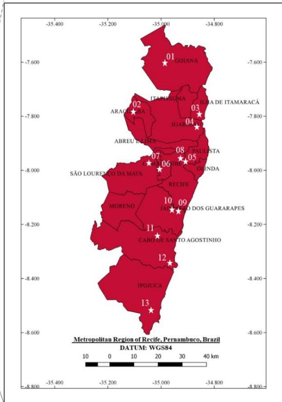  Figure 1: Location of the soils in the Metropolitan Region of Recife - Pernambuco, Brazil The characteristic climate of the region is marked by large volumes of rainfall (1,500 to 2,000 mm per year) and high temperatures $(>20^{\circ}\mathrm{C})$, according to the Agência Pernambucana de Água e Clima (APAC), a typical condition of tropical environments according to CHESWORTH et al., (2008). Most of the selected materials are from the Barreiras Geological Formation which is formed by unconsolidated sediments with diversified particle size, observing the predominance of clay and sandy clay sediments and, less frequently, sandy, and may also present ferruginous concretions and pebbles (CPRM, 2014 and Coutinho et al., 2019). In terms of pedology, the predominant soils are yellow acrisols and yellow latosols (in the Brazilian classification), which in the international soil classification system of the Food and Agriculture Organization of the United Nations (FAO) can comprehend the classes of ferralsols and acrisols. 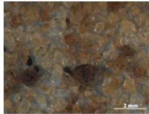They are soils that have suffered a lot from weathering processes and often present the phenomenon of natural cohesion/cementation, which is a strong pedogenetic hardening of the soil when it reaches the dry state (reversible in the wet state) due to the high concentrations of Fe hydroxides and Al oxides (CPRM, 2014; Guimarães, Silva Filho and Castro, 2021; Sousa et al., 2021; Coutinho and Sousa, 2021), as was clearly identified in the soils studied in this article (examples in Figure 2).  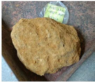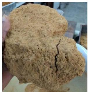 (a) 12SU-LG 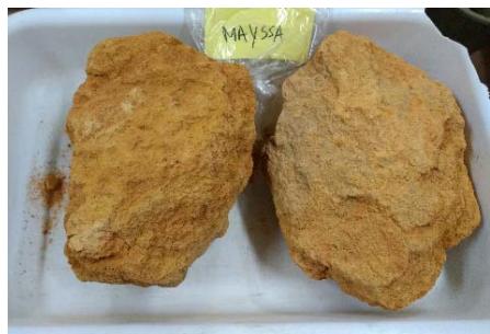 (b) 13IP-LA' Figure 2: Examples of the natural cementation of the thin tropical soils of this research ### b) Geotechnical Tests And Parameters The geotechnical parameters of the soils were obtained by physical, mechanical, chemical and mineralogical tests in the laboratory following, whenever possible, the Brazilian standards of the National Department of Transport Infrastructure (DNIT, formerly DNER). In all, 57 variables were considered, and Table 2 presents a list of the tests performed with an indication of which of the parameters obtained through them were used as the basis for the generation of soil clustering, including their respective units, as well as the standards and manuals that served as a reference for the execution of each test. Table 2: Performed tests, obtained geotechnical parameters and reference standards/manuals <table><tr><td>Test</td><td>Parameters</td><td>Standards</td></tr><tr><td>Real Particle Density</td><td>Real Particle Density (δ, g/cm3)</td><td>DNER-ME 093/94</td></tr><tr><td>Atterberg limits</td><td>Liquid Limit (LL,%), Plastic Limit (PL,%), Plasticity Index (PI,%)</td><td>DNER-ME 122/94; DNER-ME 082/94</td></tr><tr><td>Granulometric analysis (with deflocculant)</td><td>%Clay,%Silt,%Sand,%Fine Sand (%FS),%Medium Sand (%MS),% Coarse Sand (%CS),%Gravel(%Grav)</td><td>DNER-ME 051/94</td></tr><tr><td>MCT Classification</td><td>Coefficients c&#x27; and d&#x27;, e&#x27; index, Immersion Mass Loss (PMI,%), Immersion Mass Loss - specimen with optimal soil moisture (PMLwo,%)</td><td>DNER-ME 258/94; DNER-ME 256/94</td></tr><tr><td>Compaction</td><td>Apparent dry specific weight (ρdmáx, g/cm3) and optimal moisture content (w0,%)</td><td>DNIT 164/2013-ME</td></tr><tr><td>California Bearing Ratio</td><td>CBR (%) and expansion (Exp.,%) at the optimal moisture content</td><td>DNIT 172/2016-ME</td></tr><tr><td>Chemical tests</td><td>hydrogen potential in: water (pHH2O) and KCl (pHKCI), ΔpH (pHKCI - do pHH2O), Organic Matter (M.O., g.kg-1), Base saturation (V,%), Aluminum saturation (S,%), Cation Exchange Capacity (CEC, cmolcdm-3)</td><td>EMBRAPA (2017)</td></tr><tr><td>Soil-Water Characteristic Curve</td><td>Soil suction at optimal moisture contente (Swo, kPa), saturation humidity (θs,%), residual moisture (θr,%), suction obtained in the resilient module specimens (SMR, kPa) and parameters of Model&#x27;s Gitirana Jr. and Fredlund (2004) - Ψb1, Ψres1, Sres1, Ψb2, Sb, Ψres2, Sres2</td><td>ASTM D5298 - 16</td></tr><tr><td>Resilient Modulus</td><td>Resilient Modulus medium (MRmedium, MPa), regression coefficients of linear models as a function of stresses: confining stress (K1TC e K2TC) and deviator (K1TD e K2TD), Composite model parameters (K1MC, K2MC e K3MC)</td><td>DNIT 134/2018-ME</td></tr><tr><td>Permanent Deformation</td><td>Maximum permanente deformation (εp, mm) obtained under confining stress - σ3 (120 kPa) and deviator stress - σd (360 kPa), Parameters of the Guimaraes Model (2009) - Ψ1, Ψ2, Ψ3 and Ψ4</td><td>DNIT 179/2018-IE</td></tr></table> The LL and PL tests were performed both with samples previously dried in the air and destroyed (standard procedure) and without previous drying, and the parameters obtained were identified as follows: without previous drying - LL1, PL1 and PI1 and, with drying and destruction: LL2, PL2 and PI2. The test of the soil-water characteristic curve was performed using the filter paper method, with the specimen compacted on the intermediate Proctor energy and considering a drying and wetting mixed trajectory. The model adjustment parameters of Gitirana Jr. and Fredlund (2004) follow equation 1, applicable to soils with bimodal behavior commonly identified in lateritic tropical soils. The coefficients of determination $(R^2)$ obtained were all very close to 1 (>0.91) showing suitability of the model to the soil behavior of this article. $$ S _ {e} = \frac {S _ {1} - S _ {2}}{1 + (\frac {\psi}{\sqrt {\psi_ {b 1} \psi_ {r e s 1}}}) ^ {d _ {1}}} + \frac {S _ {2} - S _ {3}}{1 + (\frac {\psi}{\sqrt {\psi_ {r e s 1} \psi_ {b 2}}}) ^ {d _ {2}}} + \frac {S _ {3} - S _ {4}}{1 + (\frac {\psi}{\sqrt {\psi_ {b 2} \psi_ {r e s 2}}}) ^ {d _ {3}}} \tag {1} $$ Where: $S$ = degree of saturation; $=$ suction obtained in the laboratory test; $b$ = suction at the air inlet point; $res$ = residual suction and d1, d2, d3 = model's parameters. Mechanical compaction, CBR, resilient modulus (MR) and permanent deformation tests were performed on the intermediate Proctor energy. The equations that were used to model resilient behaviors and permanent soil deformation are indicated in Table 3. Table 3: Models used to express the resilient behavior and permanent deformation of the soils of this research <table><tr><td>References</td><td>Equation</td><td>Variables</td><td>Parameters</td></tr><tr><td>Hicks and Monismith (1970)</td><td>MR=k13k2</td><td>3</td><td>k1 and k2</td></tr><tr><td>Svenson (1980)</td><td>MR=k1dk2</td><td>d</td><td>k1 and k2</td></tr><tr><td>Macêdo (1996)</td><td>MR=k13k2dk3</td><td>3;d</td><td>k1, k2 and k3</td></tr><tr><td>Guimarães (2009)</td><td>p(%)=1302d03N4</td><td>3;d and N</td><td>1, Ψ2, 3 and 4</td></tr></table> Notation: 3 = confining stress; d = deviator stress; p(%) = Specific permanent deformation, N = number of loading cycles and, k1, k2, k3, 1, Ψ2, 3 and 4 are regression parameters, 0 = reference stress, considered with the atmospheric pressure of 100 kPa. ### c) Data Science Tools For Cluster Analysis The implementation of the codes required for the analyses was carried out in the Python programming language (version 3) available in the Anaconda virtual environment (https://www.anaconda.com/). In addition to the standard Python library, modules and functions from other libraries were used as indicated in Table 4, which explains the general objectives of each (in the application column) and in the column "functions and modules" is the specific indication of the main tools that were used. Table 4: Main Libraries, modules and functions used in the analysis with Python in this research <table><tr><td>Libraies</td><td>Application</td><td>Modules and functions</td></tr><tr><td>Pandas https://pandas.pydata.org/</td><td>Data manipulation and analysis: structures and operations to manipulate numerical tables and time series.</td><td>read_excel, drop, set_index, head, shape</td></tr><tr><td>Numpy https://numpy.org/</td><td>Data analysis: mathematical functions, random number generators, linear algebra routines, Fourier transformations, etc.</td><td>Array, arrange, mean, std, argsort</td></tr><tr><td>Scipy https://www.scipy.org/</td><td>Data modeling: fundamental algorithms for statistical functions (probability distributions, hypothesis testing, frequency statistics, correlation functions, etc.).</td><td>scipy.cluster, hierarchy, hierarchy linkage (method=&#x27;ward&#x27;, metric=&#x27;euclidean&#x27;), hierarchy.dendrogram</td></tr><tr><td>Scikit-learn https://scikit-learn.org/</td><td>Data Modeling: Machine learning algorithms, supervised and unsupervised (Classification, Regression, Clustering, Model Selection, etc.)</td><td>sklearn.preprocessing, StandardScaler, transform</td></tr><tr><td>Scikit-image https://scikit-image.org/</td><td>Image processing: functions for manipulating scientific, specific or general-purpose images, operations on Numpy matrices, manipulation of exposure and color channels, detection and segmentation of objects.</td><td>Feature</td></tr><tr><td>Imageio https://pypi.org/project/imageio/</td><td>Image manipulation: reading and writing image data, including animated images, volumetric data, and scientific formats.</td><td>imread</td></tr><tr><td>Matplotlib https://matplotlib.org/</td><td>Data presentation and exploration: creating graphs and general data visualization</td><td>plot.figure, plot.title, plotxlabel,, plotylabel, subplot, imshow</td></tr></table> For the analysis of data clusters through the hierarchical method and implementation via codes and libraries in Python, the data were standardized by applying the Z-score Normalization Method, and for this an array was created through the "array" function of the Numpy library and the functions "StandardScaler" and "transform" of the Scikit-learn library were applied. Then, to obtain hierarchical cluster of the (standardized) datasets, the hierarchy function of the Cluster module of the SciPy library was imported. The implementation was made considering Ward's linkage method and Euclidean distance. ### d) Image Comparison As a complementary analysis and a way of using data science tools for image analysis, images were separated from the fine-earth fraction of soils (in this case the material passing in sieve no. 10 and retained in no. 200) made in the Stereo Microscope Zeiss Discovery V8 in order to compare the soils to each other and to verify some similarity with the results obtained in the clustering. The mineralogy of the fraction passing in sieve no. 200 was studied by performing the X-ray Diffraction test and images of the coarse fraction of the soil (retained in sieve no. 10) were also extracted, but were not considered in the analyses of this article. In summary, the process of comparing images in Python is done by implementing a function that receives the image and processes it by transforming it into vectors. The function applied in this article was the BIC (Border-Interior Pixel Classification), which transforms and rescales the image, and finally computes two color histograms: one for the "interior" pixels and the other for the "border" pixels (edges of the image), then normalizes the histograms and concatenates them into a single vector. Vectors represent the frequencies of colors in the image, which allows, with the aid of a distance measurement, to compare images for color similarity. To make the comparison, you must set an image as a reference so that the distance of the other images related to it is calculated. In this part of the analysis, we chose to use the same distance measurement used in the cluster analysis that was the Euclidean distance. ## III. RESULTS AND DISCUSSION ### a) Geotechnical Parameters Table 5 presents part of the database of the studied soils: geotechnical classifications (TRB, USCS and MCT), MCT classification, real density, Atterberg limits, granulometry, mechanical compaction parameters, CBR (and expansion), MR, DP and chemical data. Table 6 presents the continuity of the database with parameters associated with the characteristic curve of the soils. The units of measurement of each parameter were presented in Table 2. Regarding the USCS class, five samples were classified as ML (silt soils of low compressibility), four were classified as SC (clay sand), and two as SM (silty sand). Soil 03 was classified as SM-SC and soil 13 was classified as CL (clay soil of low compressibility). Table 5: Classification database, true density, consistency limits, granulometry, compaction, CBR, expansion, MR, DP and chemical data from soils studied in this research <table><tr><td>Soil</td><td>1</td><td>2</td><td>3</td><td>4</td><td>5</td><td>6</td><td>7</td><td>8</td><td>9</td><td>10</td><td>11</td><td>12</td><td>13</td></tr><tr><td>MCT</td><td>LG'</td><td>LG'</td><td>NA'</td><td>LG'</td><td>LA'</td><td>LA'</td><td>NA'</td><td>LA'</td><td>LA'</td><td>LA'</td><td>LA'</td><td>LG'</td><td>LA'</td></tr><tr><td>TRB</td><td>A-6</td><td>A-7-6</td><td>A-4</td><td>A-6</td><td>A-6</td><td>A-6</td><td>A-6</td><td>A-4</td><td>A-4</td><td>A-7-6</td><td>A-7-5</td><td>A-6</td><td>A-6</td></tr><tr><td>USCS</td><td>ML</td><td>ML</td><td>SM-SC</td><td>SC</td><td>SC</td><td>SM</td><td>ML</td><td>ML</td><td>SM</td><td>SC</td><td>ML</td><td>SC</td><td>CL</td></tr><tr><td>d'</td><td>247</td><td>139</td><td>133</td><td>87</td><td>131</td><td>140</td><td>147</td><td>107</td><td>109</td><td>217</td><td>188</td><td>150</td><td>154</td></tr><tr><td>e'</td><td>0,94</td><td>0,62</td><td>1,19</td><td>0,93</td><td>0,62</td><td>0,62</td><td>1,16</td><td>0,84</td><td>0,91</td><td>0,87</td><td>0,84</td><td>0,81</td><td>0,81</td></tr><tr><td>c'</td><td>2,0</td><td>1,9</td><td>1,2</td><td>1,7</td><td>1,4</td><td>1,05</td><td>1,05</td><td>1,29</td><td>0,92</td><td>1,05</td><td>1,0</td><td>1,67</td><td>1,1</td></tr><tr><td>PMI</td><td>75</td><td>10</td><td>153</td><td>58</td><td>9</td><td>10</td><td>143</td><td>40</td><td>58</td><td>56</td><td>49</td><td>40</td><td>40</td></tr><tr><td>PMIwo</td><td>75</td><td>0</td><td>98</td><td>38</td><td>9</td><td>0</td><td>34</td><td>0</td><td>0</td><td>0</td><td>0</td><td>39</td><td>42</td></tr><tr><td>δ</td><td>2,63</td><td>2,67</td><td>2,65</td><td>2,63</td><td>2,64</td><td>2,67</td><td>2,69</td><td>2,70</td><td>2,68</td><td>2,68</td><td>2,68</td><td>2,67</td><td>2,68</td></tr><tr><td>LL1</td><td>32,2</td><td>33,7</td><td>22,0</td><td>26,2</td><td>30,0</td><td>28,5</td><td>32,2</td><td>34,5</td><td>27,4</td><td>27,5</td><td>33,9</td><td>27,8</td><td>28,7</td></tr><tr><td>PL1</td><td>22,8</td><td>25,9</td><td>18,0</td><td>20,3</td><td>20,4</td><td>20,4</td><td>24,4</td><td>26,5</td><td>19,3</td><td>19,8</td><td>30,4</td><td>18,7</td><td>19,8</td></tr><tr><td>PI1</td><td>9,4</td><td>7,8</td><td>4,0</td><td>5,9</td><td>9,6</td><td>8,1</td><td>7,8</td><td>8,0</td><td>8,1</td><td>7,7</td><td>3,5</td><td>9,1</td><td>8,9</td></tr><tr><td>LL2</td><td>35,6</td><td>41,3</td><td>24,1</td><td>33,4</td><td>37,9</td><td>39,9</td><td>39,9</td><td>39,5</td><td>34,7</td><td>40,5</td><td>46,6</td><td>34,8</td><td>35,9</td></tr><tr><td>PL2</td><td>25,0</td><td>27,9</td><td>17,4</td><td>21,7</td><td>23,1</td><td>26,5</td><td>28,5</td><td>32,4</td><td>24,9</td><td>25,4</td><td>30,1</td><td>21,4</td><td>24,2</td></tr><tr><td>PI2</td><td>10,6</td><td>13,4</td><td>6,7</td><td>11,7</td><td>14,8</td><td>13,4</td><td>11,4</td><td>7,1</td><td>9,8</td><td>15,1</td><td>16,5</td><td>13,4</td><td>11,7</td></tr><tr><td>%Clay</td><td>50,2</td><td>47,8</td><td>32,3</td><td>38,8</td><td>41,7</td><td>42,6</td><td>46,5</td><td>47,0</td><td>42,0</td><td>40,3</td><td>45,5</td><td>34,9</td><td>44,7</td></tr><tr><td>%Silt</td><td>14,2</td><td>19,0</td><td>5,6</td><td>6,6</td><td>4,8</td><td>5,2</td><td>13,6</td><td>19,3</td><td>5,7</td><td>8,1</td><td>6,8</td><td>4,4</td><td>8,4</td></tr><tr><td>%FS</td><td>25,3</td><td>18,7</td><td>55,9</td><td>36,2</td><td>31,5</td><td>31,1</td><td>27,3</td><td>21,8</td><td>35,3</td><td>29,9</td><td>25,9</td><td>33,6</td><td>25,5</td></tr><tr><td>%MS</td><td>10,0</td><td>11,2</td><td>6,1</td><td>17,3</td><td>18,2</td><td>20,6</td><td>12,3</td><td>11,5</td><td>16,7</td><td>20,2</td><td>20,9</td><td>25,7</td><td>20,5</td></tr><tr><td>%CS</td><td>0,3</td><td>1,2</td><td>0,1</td><td>0,8</td><td>2,1</td><td>0,6</td><td>0,3</td><td>0,3</td><td>0,3</td><td>0,8</td><td>0,9</td><td>0,9</td><td>0,9</td></tr><tr><td>%Grav</td><td>0,1</td><td>2,1</td><td>0,0</td><td>0,2</td><td>1,7</td><td>0,1</td><td>0,0</td><td>0,1</td><td>0,0</td><td>0,8</td><td>0,1</td><td>0,4</td><td>0,1</td></tr><tr><td>ρdmáx</td><td>1,79</td><td>1,75</td><td>1,97</td><td>1,91</td><td>1,94</td><td>1,88</td><td>1,78</td><td>1,69</td><td>1,90</td><td>1,87</td><td>1,86</td><td>1,94</td><td>1,86</td></tr><tr><td>W0</td><td>17,4</td><td>18,4</td><td>10,6</td><td>13,1</td><td>13,7</td><td>13,8</td><td>16,5</td><td>19,0</td><td>12,7</td><td>12,7</td><td>15,6</td><td>11,2</td><td>13,2</td></tr><tr><td>CBR</td><td>12,8</td><td>15,0</td><td>35,0</td><td>15,4</td><td>25,0</td><td>17,0</td><td>21,0</td><td>15,2</td><td>30,0</td><td>16,0</td><td>27,5</td><td>29,0</td><td>23,0</td></tr><tr><td>Exp.</td><td>0,05</td><td>0,00</td><td>0,15</td><td>0,60</td><td>0,00</td><td>0,00</td><td>0,05</td><td>0,10</td><td>0,00</td><td>0,20</td><td>0,00</td><td>0,20</td><td>0,00</td></tr><tr><td>MRmedium</td><td>416</td><td>394</td><td>865</td><td>477</td><td>425</td><td>667</td><td>557</td><td>394</td><td>507</td><td>611</td><td>487</td><td>478</td><td>689</td></tr><tr><td>K1TC</td><td>222</td><td>144</td><td>200</td><td>175</td><td>153</td><td>164</td><td>231</td><td>214</td><td>519</td><td>345</td><td>222</td><td>359</td><td>227</td></tr><tr><td>K2TC</td><td>-0,24</td><td>-0,33</td><td>-0,48</td><td>-0,32</td><td>-0,33</td><td>-0,49</td><td>-0,28</td><td>-0,2</td><td>0,01</td><td>-0,19</td><td>-0,25</td><td>-0,09</td><td>-0,34</td></tr><tr><td>K1TD</td><td>205</td><td>144</td><td>246</td><td>171</td><td>146</td><td>177</td><td>227</td><td>197</td><td>405</td><td>327</td><td>202</td><td>297</td><td>243</td></tr><tr><td>K2TD</td><td>-0,33</td><td>-0,41</td><td>-0,52</td><td>-0,42</td><td>-0,44</td><td>-0,60</td><td>-0,36</td><td>-0,29</td><td>-0,09</td><td>-0,26</td><td>-0,36</td><td>-0,20</td><td>-0,41</td></tr><tr><td>K1MC</td><td>354</td><td>282</td><td>289</td><td>295</td><td>263</td><td>168</td><td>384</td><td>342</td><td>650</td><td>462</td><td>403</td><td>483</td><td>341</td></tr><tr><td>K2MC</td><td>0,33</td><td>0,32</td><td>0,03</td><td>0,25</td><td>0,35</td><td>0,02</td><td>0,29</td><td>0,30</td><td>0,34</td><td>0,21</td><td>0,39</td><td>0,35</td><td>0,14</td></tr><tr><td>K3MC</td><td>-0,51</td><td>-0,53</td><td>-0,50</td><td>-0,52</td><td>-0,62</td><td>-0,64</td><td>-0,51</td><td>-0,43</td><td>-0,32</td><td>-0,39</td><td>-0,55</td><td>-0,43</td><td>-0,47</td></tr><tr><td>εp</td><td>6,52</td><td>6,59</td><td>2,93</td><td>7,19</td><td>1,63</td><td>6,66</td><td>4,18</td><td>3,63</td><td>0,78</td><td>3,37</td><td>3,15</td><td>1,30</td><td>6,40</td></tr><tr><td>Ψ1</td><td>0,21</td><td>0,28</td><td>0,13</td><td>0,46</td><td>0,07</td><td>0,02</td><td>0,03</td><td>0,01</td><td>0,08</td><td>0,10</td><td>0,04</td><td>0,09</td><td>0,47</td></tr><tr><td>Ψ2</td><td>-0,45</td><td>0,79</td><td>0,25</td><td>-0,51</td><td>0,07</td><td>-2,31</td><td>-1,86</td><td>-1,22</td><td>0,04</td><td>0,17</td><td>-0,53</td><td>-0,27</td><td>1,09</td></tr><tr><td>Ψ3</td><td>1,73</td><td>1,30</td><td>1,24</td><td>1,30</td><td>0,07</td><td>3,90</td><td>2,98</td><td>3,96</td><td>0,91</td><td>1,42</td><td>2,39</td><td>1,07</td><td>0,95</td></tr><tr><td>Ψ4</td><td>0,06</td><td>0,06</td><td>0,06</td><td>0,05</td><td>0,07</td><td>0,05</td><td>0,06</td><td>0,08</td><td>0,05</td><td>0,07</td><td>0,06</td><td>0,05</td><td>0,05</td></tr><tr><td>pHH2O</td><td>4,7</td><td>4,9</td><td>4,9</td><td>4,8</td><td>4,6</td><td>4,6</td><td>4,4</td><td>4,6</td><td>4,6</td><td>4,5</td><td>4,4</td><td>4,8</td><td>4,7</td></tr><tr><td>pHKCl</td><td>4,0</td><td>4,1</td><td>4,0</td><td>3,9</td><td>3,9</td><td>4,0</td><td>4,1</td><td>4,1</td><td>4,0</td><td>3,9</td><td>4,0</td><td>4,0</td><td>4,0</td></tr><tr><td>ΔpH</td><td>-0,7</td><td>-0,8</td><td>-0,9</td><td>-0,9</td><td>-0,7</td><td>-0,6</td><td>-0,3</td><td>-0,5</td><td>-0,6</td><td>-0,6</td><td>-0,4</td><td>-0,8</td><td>-0,7</td></tr><tr><td>M.O.</td><td>7,59</td><td>7,12</td><td>3,85</td><td>5,53</td><td>5,11</td><td>4,37</td><td>4,32</td><td>7,19</td><td>5,68</td><td>6,25</td><td>6,67</td><td>5,94</td><td>4,43</td></tr><tr><td>CEC</td><td>4,63</td><td>4,55</td><td>2,80</td><td>3,55</td><td>3,75</td><td>3,85</td><td>3,84</td><td>4,40</td><td>5,42</td><td>5,74</td><td>4,46</td><td>4,07</td><td>4,64</td></tr><tr><td>S</td><td>36,6</td><td>28,4</td><td>43,4</td><td>61,5</td><td>79,1</td><td>54,3</td><td>41,4</td><td>53,2</td><td>73,1</td><td>69,0</td><td>56,6</td><td>86,3</td><td>55,5</td></tr><tr><td>V</td><td>25,1</td><td>30,6</td><td>28,9</td><td>19,4</td><td>8,8</td><td>17,9</td><td>17,7</td><td>13,4</td><td>7,2</td><td>9,4</td><td>10,3</td><td>3,9</td><td>15,7</td></tr></table> In the TRB classification, three samples were classified as A-4 (non-plastic silt soils to moderately plastic), seven as A-6 (plastic clay soils), one (soil 11) as A-7-5 (PI moderate in relation to LL, and may be elastic and subject to high volume variation) and two (02 and 10) as A-7-6 (high PI in relation to LL and are subject to extremely high volume changes). According to the TRB classification, all soils of the research would present poor to bad behavior as a subbed layer of pavements, however, considering the results of the Resilient Modulus (MR) and Permanent Deformation (PD) trials, the studied soils present excellent behaviors regarding these aspects, evidencing that fine-grained tropical soils present peculiar behavior, as noted in several works already mentioned. Regarding the MCT classification, it is verified that in general, the samples further north of the metropolitan region of Recife present clayey behavior, except for sample 03 (fine sandy soil), moving to a more sandy behavior when collected in the south region (except for sample 12). It is observed that the coefficient $d'$, which is associated with the inclination of the dry branch of the Mini-MCV compaction curve (in MCT), presents important variation between the samples, indicating different behaviors. Villibor and Nogami (2009) specify that $d'$ values above 20 indicate soils of lateritic behavior and above 100 (very high) refers to the typical behavior of fine clayey sands. It is noted that most of the samples evaluated present these characteristics in this aspect and also granulometric and mineralogical. Regarding Mass Loss by Immersion $(\mathrm{PMI}_{\mathrm{wo}})$, the values obtained for specimens (CP) molded in optimum moisture were $0\%$ to almost $50\%$ of the soils, even after 24 hours of immersion. The e' index, which associates the MLI and the coefficient d', reflects the lateritic or non-lateritic behavior of the analyzed soil. Soils with low mass loss and high d' values result in lower values of e' and more evident lateritic behavior: 02, 05, 06, 08 to 13. As for the values of $c'$, which is associated with the slope of the soil deformability curve, it is understood that the higher the value of $c'$, the more deformable the soil is, since there are steeper reductions in the CP height as the blows are applied in the Mini-MCV compaction test. Thus, the soil with the highest deformability was soil 01 ( $c' = 2.0$ ) indicating the behavior of a clay soil ( $c' > 1.5$ according to Nogami and Villibor (2009)), and soil 09 presented the lowest $c'$ value showing typical behavior of non-plastic sands and silts ( $c' < 1.0$, according to Nogami and Villibor (2009)). In the permanent deformation tests, soil 09 showed the lowest deformation and soil 01 was the most notable deformation. Regarding granulometry, we stress that other parameters associated with granulometry were also considered, but deleted from the table in order to optimize the presentation of the data. The variables in this case were:% of total sand,% of passing material in sieve no. 10,% of material retained in sieve no. 10 and percentage of passing material in no. 200. All soils presented appreciable content of clay (between $32.28\%$ and $50.17\%$ ) and fine sand (between 18.66% and 55.85%), and low percentage of coarse material (retained in sieve no. 10 – between 0.12% and 3.76%). Regarding the consistency indexes (LL, PL and PI) it is observed that for all soils there was an increase in values with drying. The actual density values of the grains obtained were between 2.629 – 2.699 g/cm3 which is approximate, according to Gidigasu (1976), to the quartz mineral (2.65 to 2.66 g/cm3) and the clay mineral kaolinite (2.60 to 2.68 g/cm3), which is coherent since most of the soils studied are composed of sand and clay fractions. The results of maximum dry specific mass $(\rho_{\mathrm{dmax}}, \mathrm{g/cm}^3)$ and optimum moisture $(W_{\mathrm{or}}, \%)$ ranged between 1.69 - 1.97 g/cm3 and between 10.6 - 19%, respectively, and showed some correspondence with the granulometry. Soil 03, for example, has a large percentage of fine sand in its composition, which is reflected in the compaction curve (low optimum moisture and high specific dry mass), while soil 08, with the highest percentage of silt, compared to the other soils, presented higher moisture and lower specific mass. Six soils presented CBR values below $20\%$, which is, according to the paving manual of the Brazilian Department of Transport Infrastructure (DNIT, 2006), the minimum allowed for application in subbase layers, considering the empirical sizing method. The other soils presented values higher than $20\%$, reaching a maximum of $35\%$ (sample 03), which according to the mentioned guidelines could be recommended for subbase layer and none of the soils would be recommended for the base layer since $\mathrm{CBR} > 60\%$ is required. Regarding expansion, six soils showed an expansion of $0\%$ after 96 hours of immersion in water, and the other 7 samples showed low expansion values. The values of mean MR of all soils were above $400\mathrm{MPa}$, considered a high value for fine-grained soils, comparable to the values of boulder soils. As for permanent deformation, all soils presented low total deformation values $(\varepsilon_{\mathrm{p}}, \mathrm{mm})$ for all stress levels applied in the test. According to The National Pavement Sizing Method (MeDiNa), the sum of the contribution of all layers and subgrade to the sinking of the wheel track should be a maximum of $10 \mathrm{~mm}$ for Main Arterial Route, for example. Almost half of the soils exhibit opposite behavior in relation to the parameter $\Psi_{2}$ of the expression of permanent deformation, associated with the confining stress. Soils with negative values of $\Psi_{2}$ show a reduction in permanent deformation with increased confining stress. All values of $\Psi_{3}$ are positive indicating that the variation of the deviation stress increases permanent deformation, which is expected. The pH measurement reflects the active acidity of the soil, and the results obtained (< 5) represent soils with high acidity, which is expected for lateritic soils. Specifically in water, values between 4.4 and 4.7 were obtained indicating the presence of exchangeable aluminum (Sobral et al., 2015), which suggests possible gains in chemical stabilization processes. $\Delta \mathsf{pH}$ is associated with the predominance of clay minerals such as kaolinite and illite, (Farias, 2012 and Camapum de Carvalho et al., 2015). The CEC presented low values (between 2.8 – 5.74 $\mathrm{cmol_c dm^{-3}}$ ) indicating predominance of 1:1 clay such as kaolinite (Gidigasu, 1976; Das, 2008 and Sobral et al., 2015). Regarding Organic Matter (OM), all soils have a low content ( $< 15\mathrm{g.kg^{-1}}$ ) according to Prezotti (2013). For all soils, the percentage of base saturation ( $V$,%) is considered "low" ( $< 50\%$ ) according to Prezotti, 2013). Aluminum saturation ( $S$,%) was in the "low" class ( $< 50\%$ ) in soils 01, 02, 03 and 07, "middle" class ( $50\%$ - $70\%$ ), in 04, 06, 08, 10, 11 and 13, and, "high" class ( $>70\%$ ) in soils 05, 09 and 12, according to Prezotti, (2013). Table 6: Data of the characteristic curve of the studied soils (Continuation of the database in Table 5) <table><tr><td>Soil</td><td>SWo</td><td>θs</td><td>θr</td><td>SMR</td><td>Ψb1</td><td>Ψres1</td><td>Sres1</td><td>Ψb2</td><td>Sb</td><td>Ψres2</td><td>Sres2</td></tr><tr><td>01</td><td>200</td><td>20,58</td><td>1,47</td><td>198,59</td><td>3,5</td><td>5,0</td><td>0,84</td><td>10000</td><td>0,82</td><td>26800</td><td>0,02</td></tr><tr><td>02</td><td>800</td><td>20,67</td><td>0,00</td><td>760,23</td><td>3,0</td><td>6,0</td><td>0,89</td><td>7500</td><td>0,85</td><td>22500</td><td>0,08</td></tr><tr><td>03</td><td>30</td><td>34,34</td><td>0,06</td><td>1071,43</td><td>2,5</td><td>16,0</td><td>0,70</td><td>8000</td><td>0,62</td><td>21500</td><td>0,02</td></tr><tr><td>04</td><td>30</td><td>17,64</td><td>0,00</td><td>487,86</td><td>4,0</td><td>5,5</td><td>0,74</td><td>10000</td><td>0,59</td><td>23000</td><td>0,03</td></tr><tr><td>05</td><td>300</td><td>14,35</td><td>0,26</td><td>434,80</td><td>3,4</td><td>6,5</td><td>0,78</td><td>8700</td><td>0,72</td><td>27000</td><td>0,03</td></tr><tr><td>06</td><td>50</td><td>29,31</td><td>0,99</td><td>372,62</td><td>4,8</td><td>6,5</td><td>0,84</td><td>18000</td><td>0,77</td><td>36000</td><td>0,10</td></tr><tr><td>07</td><td>6</td><td>23,60</td><td>1,01</td><td>430,23</td><td>6,0</td><td>9,0</td><td>0,89</td><td>14000</td><td>0,83</td><td>20000</td><td>0,05</td></tr><tr><td>08</td><td>100</td><td>22,26</td><td>0,00</td><td>485,99</td><td>3,8</td><td>10,0</td><td>0,91</td><td>12000</td><td>0,87</td><td>48000</td><td>0,07</td></tr><tr><td>09</td><td>400</td><td>13,49</td><td>0,26</td><td>1088,10</td><td>1,2</td><td>11,0</td><td>0,75</td><td>14000</td><td>0,72</td><td>30000</td><td>0,04</td></tr><tr><td>10</td><td>25</td><td>23,91</td><td>0,45</td><td>1527,01</td><td>2,1</td><td>20,0</td><td>0,74</td><td>15000</td><td>0,66</td><td>25000</td><td>0,04</td></tr><tr><td>11</td><td>40</td><td>33,60</td><td>0,17</td><td>1673,32</td><td>3,8</td><td>20,0</td><td>0,79</td><td>13500</td><td>0,71</td><td>22500</td><td>0,04</td></tr><tr><td>12</td><td>1000</td><td>17,20</td><td>0,00</td><td>1147,13</td><td>2,0</td><td>11,0</td><td>0,69</td><td>5500</td><td>0,66</td><td>24000</td><td>0,04</td></tr><tr><td>13</td><td>40</td><td>26,85</td><td>0,60</td><td>275,91</td><td>3,5</td><td>6,5</td><td>0,73</td><td>13800</td><td>0,65</td><td>30000</td><td>0,04</td></tr></table> Table 6 presents the results of the modeling of the soil-water characteristic curves. The characteristic curves of the studied soils present high suction values and air intake points, since the more weathered the soil, the higher the presented suction values are (Boszczowski and Ligocki, 2012). The shape of the curves suggests a bimodal behavior, indicating that both micropores and macropores control water inlet and outlet flows (Feuerharmel et al., 2006). The high suction values obtained are also similar to those obtained by Marinho and Stuermer (2000) when they studied a mature residual soil of Gnaisse (45% clay), compacted in normal and modified Proctor energies, obtaining air intake values ranging between 1000 and 2000 kPa and residual suction of 15,000kPa. ### b) Cluster Analysis The dendrogram created by processing the codes in Python resulted in the hierarchical structure presented in Figure 3. Seeking to understand how the algorithm effectively grouped the data, a top-down dendrogram analysis was carried out, i.e., noting which geotechnical variable or variables may have been used as a soil divider in each Cluster. For this, three cut-off points were defined in the dendrogram, as highlighted in the figure, and the clusters created were identified. It is emphasized that the clusterization obtained went through a much more complex process than is described here, since more than fifty geotechnical attributes were considered. 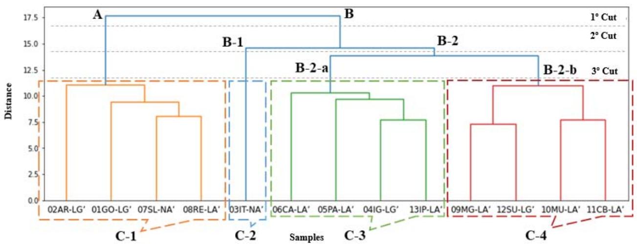 Hierarchical clustering of the soils of this research Ward Method and Euclidean Distance Figure 3: Analysis of the dendrogram of the hierarchical clustering of the soils of this research Initially, in the first cut-off point, the algorithm divided the soils into two large groups (A and B), which may have been formed considering the results of the compaction test (optimum moisture and maximum dry apparent specific mass), since, as can be seen in the graph of Figure 4, there is a clear division of these groups through the compaction curves. Thus, it is observed that group A is composed of soils with higher values of optimum moisture $(\mathrm{Wo} > 16\%)$ and lower values of $\rho_{\mathrm{dmax}} (< 1.8\mathrm{g/cm^3})$ and group B of soils with $\mathrm{Wo} < 16\%$ and $\rho_{\mathrm{dmax}} > 1.8\mathrm{g/cm^3}$. It was also noted that group A is composed entirely of USCS's ML class soils that take into account LL and PI.  Figure 4: Division of groups A and B by the soil compaction curves of this research In the second cut-off point, it is observed that group B is subdivided into two other groups (B-1 and B-2), while group A remains the same (showing that the soils of this group have more homogeneous characteristics than the soils of group B). This part of the clustering may have been made based on the granulometric composition, especially by the silt and fine sand fractions of the soils. The subdivision of group B into B-1 and B-2 was due to the high% of fine soil sand 03IT-NA' (55.85%), which differentiated it from the other soils of the group, as can be seen in the graph of Figure 5. 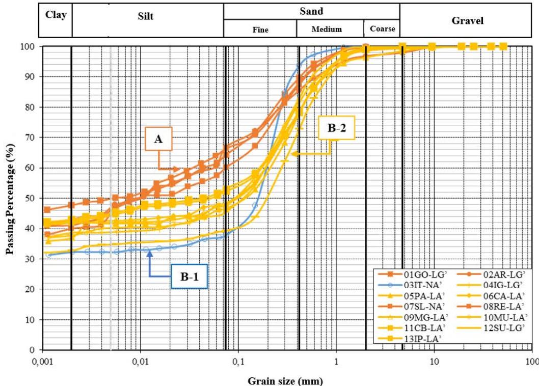 Figure 5: Division of groups A, B1 and B2 by the granulometric curves In the third and last cut-off point, group A again remained homogeneous. Because group B-1 was composed only of soil 03IT-NA', it also had no alterations (and will not have). group B-2, however, was subdivided into two subgroups (B-2-a and B-2-b), whose division may have been carried out as a function of the organic matter content found in the soils, as shown in Figure 6 (B-2-a: O.M. between 4.37 - 5.53 g/kg; B-2-b: 5.68 - 6.67 g/kg), but may also be associated with the behavior of several other variables that, despite presenting a certain "overlap" of values between groups tend, to present lower or higher results such as: $\varepsilon_{\mathrm{p}}$ - B-2-a: between $1.63 - 7.19 \mathrm{~mm}$; B-2-b: $0.78 - 3.37 \mathrm{~mm}$; $\psi_{\mathrm{b1}}$ - B-2-a: between $3.4 - 4.8 \mathrm{kPa}$; B-2-b: $1.2 - 3.8 \mathrm{kPa}$. 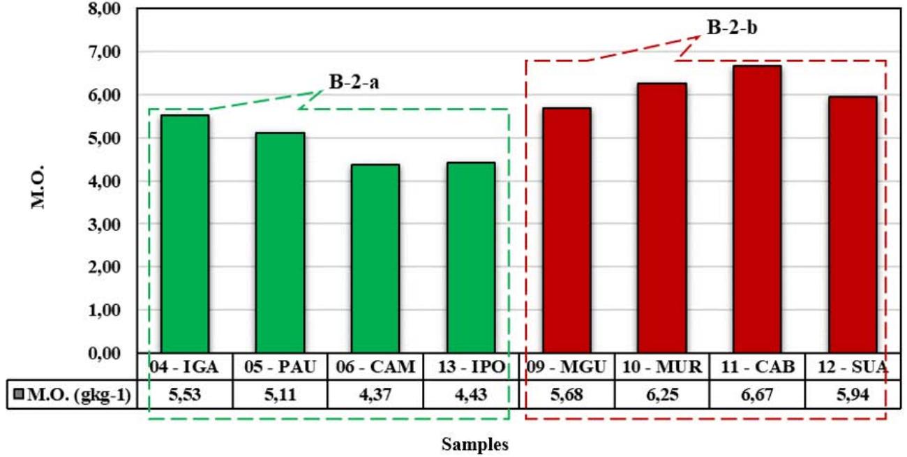 Figure 6: Division of groups B-2-a and B-2-b considering the organic matter content of the soils of this research The final interpretation of the group allows the division of the studied soils into four different clusters (C-1 to C4) in the dendrogram, cluster 1 (C-1) composed of 4 soils of group A (01GO-LG', 02AR-LG', 07SL-NA' and 08RE-LA'), Cluster 2 (C-2) composed of the soil of group B-1 (03IT-NA'), Cluster 3 (C-3) formed by 4 soils of subgroup B-2-a (04IG-LG', 05PA-LA', 06CA-LA' and 13IP-LA') and Cluster 4 (C-4) composed of 4 soils of subgroup B-2-b (09MG-LA', 10MU-LA', 11CB-LA' and 12SULG'). From each cluster, greater similarities were identified between some pairs of soils, namely: c-1 - 07SL-NA' and 08RE-LA', C-3 - 04IG-LG' and 13IP-LA' and C-4 - 10MU-LA' and 11CB-LA'. Soils 07SL-NA' and 08RE-LA', despite being of different MCT classes, are of identical USCS class and have similar values of liquidity limit,%clay, pHKCl, δ, εp and Sb. Soils 04IG-LG' and 13IP-LA', though also of different MCT classes, are of the same TRB class (A-6) and have analogous values of PI, optimum moisture, K2TC, K2TD, εp, U'b1 and Sres1. The soils 10MU-LA' and 11CB-LA' are of the same MCT class with similar values of c', e',% silt, PI, εp and Ψres1. It was also observed that the classification of aluminum saturation indicated by Prezotti (2013) may also be related to general soil grouping, since only one soil in each saturation class (low, medium and high) is distant from the formed group, which is certainly due to the other variables considered. 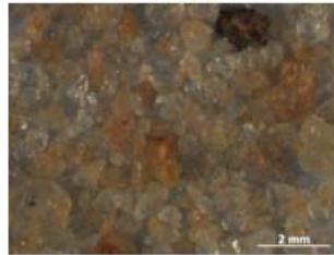### c) Stereo Mircroscope Image Comparison Figures 7, 8 and 9 present the images that are most similar to the images of the 04IG-LG', 08RE-LA' and 12SU-LG' samples, respectively (a sample of each cluster obtained in the hierarchical cluster, with the exception of the cluster composed of the sample 03IT-NA because it is a group with a single element). The numbers presented next to each ranked image refers to the Euclidean distance in relation to the reference image. The soils with color distribution most similar to soil 04IG-LG' are soils 07SL-NA', 13IP-LA', 11CB-LA', 10MU-LA' and 03IT-NA', and it is noted that, with the exception of sample 07SL-NA', the indicated soils are part of the same large hierarchical group (B) and, in addition, the 13IP-LA' soil coincides with the soil closest to 04IG-LG' in cluster C3/B-2-a. Visual similarity regarding the predominance of quartz particles is noted. 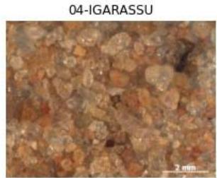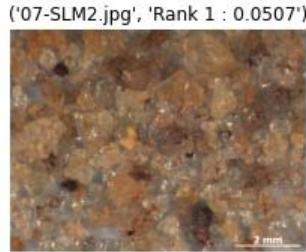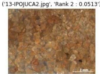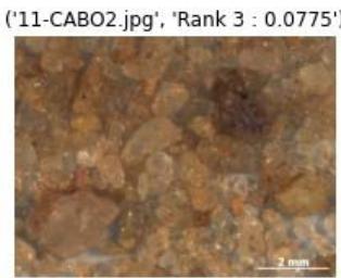Out\[41\]: (-0.5, 1387.5, 1039.5, -0.5)     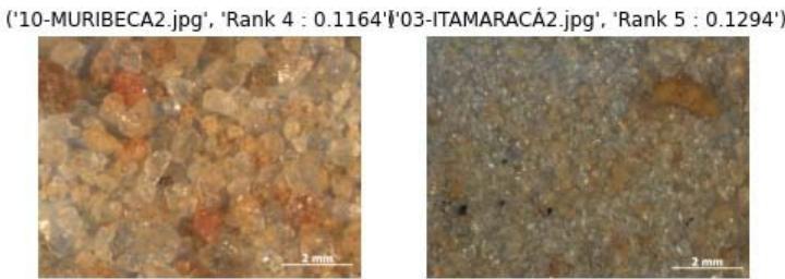 Figure 7: Images similar to sample image 04IG-LG, fine fraction The soils with color distribution most similar to soil 08RE-LA' are soils 01GO-LG', 06CA-LA', 02AR-LG', 09MG-LA' and 12SU-LG', and it is noted that with the exception of sample 06CA-NA', the two closest soils are Out\[35\]: (-0.5, 1387.5, 1039.5, -0.5) soils 01GO-LG' and 02AR-LG' which are part of the same large hierarchical group (A/Cluster C1). Visual similarity is also noted in relation to the presence of iron oxides (limonite).  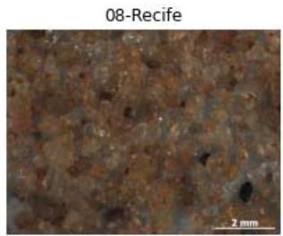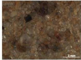 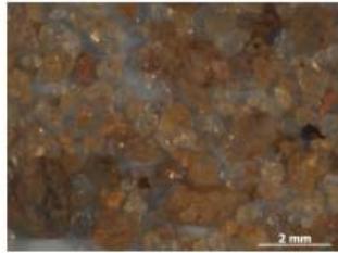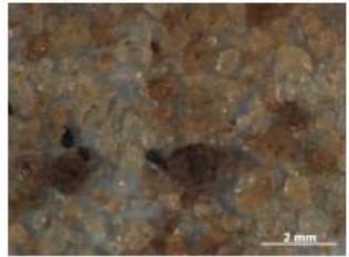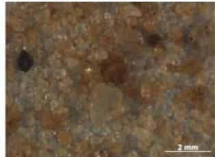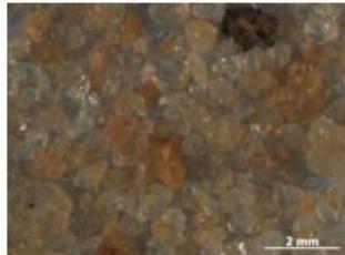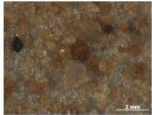('01-GOIANA2.jpg', 'Rank 1: 0.0559'X'06-CAMARAGIBE2.jpg', 'Rank 2: 0.0985')   ('02-ARACOIABA2.jpg', 'Rank 3: 0.16259-M.GUARARAPES2.jpg', 'Rank 4: 0.1736112-SUPE2.jpg', 'Rank 5: 0.1993')   Figure 8: Images similar to sample image 08RE-LA', fine fraction Out\[48\]: (-0.5, 1387.5, 1039.5, -0.5) ('09-M.GUARARAPES2.jpg', 'Rank 1: 0.0273D2-ARAÇOIABA2.jpg', 'Rank 2: 0.0606')  12-SUAPE2   ('05-PAULISTA2.jpg', 'Rank 3:0.0913'('06-CAMARAGIBE2.jpg', 'Rank 4:0.1078'('01-GOIANA2.jpg', 'Rank 5:0.1688')   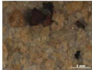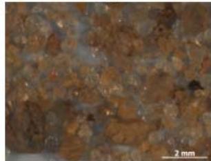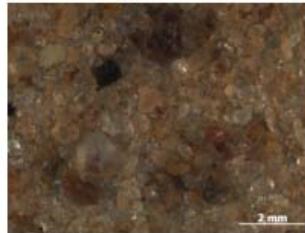 Figure 9: Images similar to the 12SU-LG sample image,' fine fraction of this research The soils with color distribution most similar to soil 12SU-LG' are soils 09MG-LA', 02AR-LG', 05PA-LA', 06CA-LA' and 01GO-LG'. It is noted that the closest soil (09MG-LA') coincides with the result of the cluster analysis, and, with the exception of soils 01GO-LG' and 02AR-LG', the other soils indicated as close are part of the same large group and subgroup (B and B-2). In view of the obtained results, the comparison of soils through images using the techniques of data science can be considered promising, since the obtained results were near the cluster obtained with cluster analysis. The results using these two techniques, even though the same parameters were not used, showed correspondence between the mineralogical characteristics visualized in the images (iron oxides, rock fragments, quartz grains, etc.) with the results of geotechnical tests. The few variations found can be attributed to the methods themselves, since each technique used can provide different results (distance measurements, linkage methods, image descriptor, etc.). As mentioned in the topic of Materials and Methods, for the acquisition of images, a Stereo Microscope Zeiss Discovery V8 available in the Paleontology laboratory of the Department of Geology of Federal University of Pernambuco was used. Although not trivial, it is believed that access to this type of equipment in universities is not very difficult, since it is an essential equipment in geology laboratories, biology and medicine. It can be noted that to use the Data Science tools presented here, it is not required that the images be obtained by this type of specific microscope, in fact, the important thing is that the images are of good quality and that they are obtained using minimum standards (process of obtaining samples, fraction of material, approximations, etc.) in order to obtain reliable results. ## IV. CONCLUSION The thirteen tropical soils of fine granulation examined in this study, originating from the northeastern region of Brazil, were characterized as materials with physical and mechanical behavior varying between clayey and sandy, having been labeled into different classes of fine soils according to the considered Classification systems (MCT, TRB and USCS). They presented high values of resilient modulus, low levels of permanent deformation, unsaturated behavior of the bimodal type in all soil-water characteristic curves, as well as chemical and mineralogical characteristics indicative of typically lateritic soils. Multivariate analyses, such as cluster analysis applied in this article, consider three or more variables to characterize the behavior of the analyzed object, so it is understood that several geotechnical parameters were used at the same time to form the groups with the most homogeneous characteristics. In this sense, other clusters were tested excluding, for example, the parameters of the two-dimensional models of resilient behavior (keeping only those associated with the composite model that presented the best framework for most soils), and it was observed that by excluding only the data associated with the model, or due to the deviation stress or the confining stress, there is no change in the dendrogram, however, by removing all the parameters associated with the two models, a dendrogram with another cluster structure is obtained, evidencing the association that the algorithm makes between the many variables. Still, it was possible to notice that the mechanical characteristics of soil compaction $(\rho_{\mathrm{dmax}}$ and $W_{0}$ ) were decisive for the initial division of the groups, as well as the granulometry (mainly the percentage of silt). The chemical classification of aluminum saturation (S,%) indicated by Prezotti (2013) also showed a relationship with the clustering of the soils, indicating that the clustering considered, in fact, different types of characteristics of fine-grained tropical soils (physical, mechanical and chemical). It was also noted that soils with mechanical clayey behavior (higher optimum moisture and lower dry apparent density) showed a more homogeneous behavior forming a cluster composed entirely of soils of the ML class (from the USCS classification, which is based on the LL and the PI) and with very similar characteristics of granulometry (percentage of silt and fine sand), in addition to the geotechnical compaction characteristics indicated. In the group formed by soils of sandy behavior (B), the subdivision was done also by considering, in addition to the parameters considered in group A, the organic matter content, and it was noticed that the association between several other variables was also considered, since there was a tendency towards lower or higher values in some parameters, for example: in terms of total permanent deformation $(\varepsilon_{\mathrm{p}})$ in subgroup - B-2-a: soils with $\varepsilon_{\mathrm{p}}$ larger $(1.63 - 7.19\mathrm{mm})$ than those of group B-2-b $(\varepsilon_{\mathrm{p}}$ between $0.78 - 3.37\mathrm{mm}$ ) were included; the suction in the first at the air intake point associated with macropores $(\psi_{\mathrm{b1}})$ tended to be slightly higher in the soils of group B-2-a $(3.4 - 4.8\mathrm{kPa})$ when compared to B-2-b $(1.2 - 3.8\mathrm{kPa})$. The recognition of the similarity between some pairs of soils proved the validity of the hierarchical clustering technique since several variables with similar values were identified between them, even though they were of a different nature (physical, chemical and mechanical), the most recurrent being: LL, PI,%Clay,% silt, c', e', pHKCl, δ, Sb, Ψb1, Ψres1, Sres1, Wo, K2TC, K2TD, εp. The comparison of images applying the techniques of data science also corroborated, since satisfactory results were obtained, congruent with those obtained in cluster analysis, with rare exceptions. It is assumed, therefore, that there is correspondence between the mineralogical characteristics visualized in the images (iron oxides, rock fragments, quartz grains, etc.) with the results of geotechnical tests. Finally, it is concluded that the application of cluster analysis by hierarchical method, as well as the comparison of microscopic images, using the tools of Data Science, showed useful techniques and tools for the cluster analysis of fine-grained tropical soils since it portrayed the similarity of behavior of different soils considering several geotechnical aspects. ### ACKNOWLEDGEMENTS The authors thank the Foundation for Science and Technology of Pernambuco (FACEPE) for the financial support (doctoral scholarship to the first author) and incentive to carry out this research. The research was carried out through the INCT REAGEO Project through the partnership signed between GEGEP (Geotechnical Engineering Group of Disasters and Plains) of THE PPGEC of UFPE (Federal University of Pernambuco) and the Geotechnics Laboratory of COPPE/UFRJ (Federal University of Rio de Janeiro).

Generating HTML Viewer...

References

42 Cites in Article
R Boszczowski,L Ligocki (2012). Chapter 8: Características Geotécnicas dos solos residuais de Curitiba e RMC. In Twin Cities -Solos das Regiões Metropolitanas de São Paulo e Curitiba.
José Camapum De Carvalho,Lilian De Rezende,Fabricio Cardoso,Lêda Lucena,Renato Guimarães,Yamile Valencia (2015). Tropical soils for highway construction: Peculiarities and considerations.
Chun-Houh Chen,Wolfgang Härdle,Antony Unwin (2007). Handbook of Data Visualization.
Roberto Coutinho,Mayssa Da Silva Sousa (2021). Analysis of the Applicability of USCS, TRB and MCT Classification Systems to the Tropical Soils of Pernambuco, Brazil, for Use in Road Paving.
Roberto Coutinho,Marilia Silva,Amabelli Santos,Willy Lacerda (2019). Geotechnical Characterization and Failure Mechanism of Landslide in Granite Residual Soil.
Cprm (2014). Geodiversidade do estado de Pernambuco.
A Dalla Roza,L Motta (2018). Classificação MCT com relação ao comportamento resiliente e deformação permanente em solos do Mato Grosso.
Braja Das (2008). Advanced Soil Mechanics.
W Farias (2012). Processos Evolutivos de Intemperismo Químico e Sua Ação no Comportamento Hidromecânico de Solos do Planalto Central.
C Feuerharmel,Wyy Gehling,Avd Bica (2006). The Use of Filter-Paper and Suction-Plate Methods for Determining the Soil-Water Characteristic Curve of Undisturbed Colluvium Soils.
David Forsyth (2018). Probability and Statistics for Computer Science.
I Frank,R Todeschini (1994). The data analysis handbook.
M Gidigasu (1976). Laterite soil engineering: Pedogenesis and engineering principles.
G Gitirana,D Fredlund (2004). Soilwater characteristic curve equation with independent properties.
Dayse Nascimento,Carolina Chagas,Norma Souza,Graciete Marques,Fernanda Rodrigues,Clicia Cunha,Deborah Santos,Patricia Silva (2016). Experiência Cotidiana: a Visão da Pessoa com Estomia Intestinal.
A Guimarães (2009). Um Método Mecanístico Empírico para Previsão da Deformação Permanente em Solos Tropicais Constituintes de Pavimentos.
Antonio Guimarães,Laura Da Motta,Carmen Castro (2019). Permanent deformation parameters of fine – grained tropical soils.
A Guimarães,J Silva Filho,C Castro (2021). Contribution to the use of alternative material in heavy haul railway sub-ballast layer.
W Hardle,L Simar (2015). Applied Multivariate Statistical Analysis.
Charles Harris,K Millman,Stéfan Van Der Walt,Ralf Gommers,Pauli Virtanen,David Cournapeau,Eric Wieser,Julian Taylor,Sebastian Berg,Nathaniel Smith,Robert Kern,Matti Picus,Stephan Hoyer,Marten Van Kerkwijk,Matthew Brett,Allan Haldane,Jaime Del Río,Mark Wiebe,Pearu Peterson,Pierre Gérard-Marchant,Kevin Sheppard,Tyler Reddy,Warren Weckesser,Hameer Abbasi,Christoph Gohlke,Travis Oliphant (2020). Array programming with NumPy.
T Hastie,R Tibshirani,J Friedman (2009). The elements of statistical learning: data mining, inference, and prediction.
Caroline Lima,Laura Motta,Antônio Guimarães (2017). Estudo da deformação permanente de britas granito-gnaisse para uso em base e sub-base de pavimentos.
C Lima,L Motta,Da,F Aragão,A Guimarães (2020). Mechanical characterization of fine-grained lateritic soils for mechanistic-empirical flexible pavement design.
Fernando Marinho,Mônica Stuermer (2000). The Influence of the Compaction Energy on the SWCC of a Residual Soil.
Mayssa Alves Da,Silva Sousa,Roberto Quental Coutinho,& Laura,Maria Goretti Da Motta (2021). Analysis of the unsaturated behaviour of compacted lateritic fine-grained tropical soils for use in transport infrastructure, Road Materials and Pavement Design.
J Medina,E Preussler (1980). Características Resilientes de Solos Em Estudos de Pavimentos. SOLOS E ROCHAS.
J Medina,L Motta (2015). Mecânica dos Pavimentos.
Jean Metz (2006). Interpretação de clusters gerados por algoritmos de clustering hierárquico.
K Millman,Michael Aivazis (2011). Python for Scientists and Engineers.
J Nogami,D Villibor (1991). Use of lateritic fine-grained soils in road pavement base courses.
J Nogami,D Villibor (1995). Pavimentação de Baixo Custo com Solos Lateríticos.
F Pedregosa (2011). Getting Started with Scikit‐learn for Machine Learning.
Maria Assis,Renata Cançado,Robson Rezende,Liliana Barros,Tânia Grão-Velloso,Danielle Camisasca (2013). Prevalência de lesões orais numa população pediátrica Brasileira.
L Sobral,M Barreto,A Silva,J Anjos (2015). Manual de emergencias cardiologicas: guia prático para estudantes de medicina.
Mayssa Sousa,Antonio Guimarães,Carmen Castro (2016). Características geotécnicas e resilientes de solos de taludes ao longo do traçado da Estrada de Ferro Carajás para fins de utilização em infraestrutura de transportes.
M Svenson (1980). Ensaios triaxiais dinâmicos de Solos argilosos.
Jake Vanderplas (2016). Appendix A: Working with Data.
D Villibor,J Nogami (2009). Pavimentos econômicos: Tecnologia do uso dos solos finos lateríticos.
Explore published articles in an immersive Augmented Reality environment. Our platform converts research papers into interactive 3D books, allowing readers to view and interact with content using AR and VR compatible devices.
Your published article is automatically converted into a realistic 3D book. Flip through pages and read research papers in a more engaging and interactive format.
Our website is actively being updated, and changes may occur frequently. Please clear your browser cache if needed. For feedback or error reporting, please email [email protected]
Thank you for connecting with us. We will respond to you shortly.