## I. INTRODUCTION Volatile regions have always attracted many people worldwide because of the high fertility of their soils (Diana et al., 2019). However, human proximity to volcanoes can lead to several health problems as a consequence of the chronic exposure to the materials released from the volcanic activity. An element often found in elevated concentrations in volcanic regions is fluorine. Although fluoride is recognized to have a beneficial effect on the rate of occurrence of dental caries when ingested in small amounts, its excessive intake results in a widespread but preventable pathological disease called fluorosis (Dey and Giri, 2015) While skeletal fluorosis, the most severe form of fluorosis, requires a chronic exposure to high concentrations of fluoride in water $(4 - 8\mathrm{mg / L})$ dental fluorosis occurs after shorter periods of exposure to fluoride in lower concentrations $(1.5 - 2.0\mathrm{mg / L})$. In some volcanic regions, where exposure to elevated amounts of fluoride is persistent, biomonitoring programs are fundamental (Garcia and Borgnino, 2015). In the present world pollution scenario, a comprehensive knowledge of pollutants and their adverse effects on the ecosystem are required for selection of a workable monitoring and conservation technique (Munzi et al., 2012; Ahmad et al., 2007). The increasing awareness of the potential hazards and impact of air pollution on the health of human populations, forest decline, climate change and loss of agricultural productivity, for example, has been a cause of increasing public concern throughout the world (Smodis, 2007). This has highlighted the need for continuous monitoring of the levels of pollutants in the environment (Garty et al., 2002). Environmental monitoring approaches that are cheap, can be used anywhere, and respond to many kinds of airborne pollutants are needed to fingerprint the pollutant sources and their dispersion pattern (Larsen et al., 2007). A comprehensive approach to reduce the impacts of pollution and climate change, an approach that decreases emissions across all sectors and enhances the adaptive capacity of all nations with economic reflections is needed (Pinhoa et al., 2012). Lichens emerge as the key answer to this monitoring problem and are the flora of choice for monitoring studies (Notcutt and Davis, 1989). They obtain their nutrients directly from the atmosphere and their chemical composition therefore holds the promise of becoming a natural or 'green' technique for monitoring the health of the environment around passively degassing volcanoes and industries. Bioaccumulation in lichen thalli has been used as a major tool for assessing air quality in volcanic and industrial areas (Bennett, 2006). They are extremely valuable in environmental monitoring since they exist worldwide and are sensitive to many different kinds of pollutants (Brodeková et al., 2006). They are slow growing; do not shed parts and are perennial pioneer plants commonly described as sentinel organisms (Loppi et al., 2002). They are good bio-accumulators of heavy metals and trace elements and can be transplanted where they do not occur in nature (Llop et al., 2012). Lichens are mutual symbiosis between fungi with an algal and/or a cyanobacterial partner (Morris and Purvis, 2007). The success in lichenization is attributed to a genetic combination resulting from metabolic biomolecules and influenced by environmental factors (Jatinder et al., 2012). This process has created unique characteristics in lichens such as the unique anatomical (absence of roots, stomata, vascular tissues and cuticle) and physiological (poikilohydr and absorbance of nutrient from general thallus surface from the atmosphere. These peculiarities, allow lichens to grow in all sorts of terrestrial habitats comprising $8\%$ of vegetation. According to Lawrey (1986), lichens produce a wide array of more than 1000 unique secondary metabolites (depsides, depsidones, $\beta$ -orcinoldibenzyl esters, and xanthones, usnic acid and pulvinic acid derivatives, for example) as adaptations for life in marginal habitats. These secondary metabolites assist to maintain the lichen symbiotic association and compete with organisms sharing the same niche (Culberson and Culberson, 2001). Another characteristic stress-resistance mechanism is the accumulation of melanin and oxalate crystals in their thallus, which provide a crystal layer on the thallial surface making lichens tolerant to extreme environments and good bioaccumulators of atmospheric substances (Hess et al., 2008). Most lichens are tolerant to high concentrations of atmospheric pollutants well beyond levels necessary for their physiological requirement by sequestrating and accumulating varied oxalate crystals (Garty et al., 2002; Bjerke et al., 2002; Chen et al., 2000). The aggregates of these oxalate crystals disintegrate and provide a crystal layer on the thallial surface making lichens good bioaccumulators. Since lichens do not shed parts (Walker et al., 2003; Monge-Najera et al., 2002), and bioaccumulate pollutants safely in their thalli over time, pollutants levels can be professionally determined quantitatively by chemical analysis of species and qualitatively by observing species diversity, abundance and distribution (Jovans, 2008). With their indiscriminate ability to absorb and bio-accumulate both nutrients/pollutants from the atmosphere, elevated concentrations of certain elements in lichens are a sure sign of atmospheric deposition (van Herk, 1999). Lichens can be used as bio-monitors of pollutants by quantifying the amount of trace element(s) accumulated within them over time (Srivastava et al., 2015, Bargagli, 2016). They have been used to assess deposition and air quality in hundreds of studies fluoride emissions from volcanoes and the natural occurrence of excessive amounts of fluoride in drinking water have affected the health of humans and livestock for centuries, if not millennia. Although sometimes of anthropogenic origin, high levels of fluorine are generally related to natural sources. Volcanic emissions of fluorine take the form of either sluggish permanent release from quiescent volcanoes (passive degassing) or rarer but more impacting discharges during short-lived volcanic eruptions (Schwandner et al., 2004 Linhares et al., 2017). It has been estimated that passive degassing, like that existing at Mt. Etna (Italy) and Masaya (Nicaragua) volcanoes, accounts for about $90\%$ of the volcanic fluorine release. The influence of these emissions on the surrounding environment and in particular on vegetation has been investigated by several authors (Nelson and Wheeler, 2016). Little or no bio-accumulation and monitoring work have been carried out on the active Mt. Cameroon. Mount Cameroon volcano with a return period of 20 years (Suh et al., 2003), has been the most frequent erupted volcano in West Africa, with eight eruptions in the last 100 years (1909, 1922, 1925, 1954, 1959, 1982, 1999 and 2000). It constantly releases various constituents into the environment during active eruptions and even in quiescent degassing periods (Suh et al., 2008). These researchers reported that, Mt. Cameroon basanites melt inclusions has shown high levels of carbon dioxide with a concentration of $967\mu \mathrm{g} / \mathrm{g}$, sulphur $2400\mu \mathrm{g} / \mathrm{g}$, chlorine $1270\mu \mathrm{g} / \mathrm{g}$ and fluorine $1530\mu \mathrm{g} / \mathrm{g}$. In spite of these findings, there is little knowledge of lichens toxic levels and remediation of the high levels of halides release from this volcano. The objective of this paper was to determine the concentration levels of some halogens and identify potential lichens species that can be used as appropriate bio-accumulators of halide toxicity for Mt. Cameroon degassing volcano. ## II. MATERIALS AND METHODS ### a) Description of the Study Area ## i. Location The study area (Fig.1) is the active MC volcano located in the coastal belt of the Gulf of Guinea, South West Region of Cameroon. It lies between Latitudes $3^{\circ}57'$ to $4^{\circ}27'\mathrm{N}$ and Longitudes $8^{\circ}58'$ to $9^{\circ}24'\mathrm{E}$ (Suh et al., 2003). It is the highest peak in West Africa, is of volcanic origin and rises from the Atlantic Ocean to a height of $4100\mathrm{m}$. It covers a surface area of about $1750\mathrm{km}^2$ (DeLancey and Mark, 2000).  Fig. 1: Topographic features of Mt. Cameroon and location of sampling sites mentioned in the text. ### b) Sample Sites The survey sites were divided into Northern and Southern contrasting flanks following wind direction and ash fall trends from various eruptions. The northern flank was called the leeward and southern flank was called the windward. Out of the eight sites selected on the two flanks, four were on the leeward flank (Lower Buea, Upper Buea, IRAD-Ekona and Ekona-Mbenge) and four from the windward flank (Batoke, Bakingili, Idenau and Bomana). Lower Buea on the leeward flank comprises of University of Buea campus, Great Soppo, and Sasse. Some species were collected from control area of Mamfe (5.7512° N - 9.3146° E) about 270 km from Mt. Cameroon. The survey was also done based on altitudinal levels which ranged between 3 to $2178\mathrm{m}$ above sea level (Table 1). The altitudinal levels were divided into three (low, mid and high) ranges. Table 1: Altitudinal ranges of sampling sites. <table><tr><td>Altitude</td><td>Range(m)</td><td>Sites</td></tr><tr><td rowspan="4">Low</td><td rowspan="4">3 -499</td><td>IRAD-Ekona</td></tr><tr><td>Batoke</td></tr><tr><td>Bakingili</td></tr><tr><td>Idenau</td></tr><tr><td rowspan="3">Mid</td><td rowspan="3">500-1000</td><td>Ekona-Mbenge</td></tr><tr><td>Lower Buea</td></tr><tr><td>Bomana</td></tr><tr><td>High</td><td>&gt;1000</td><td>Upper Buea</td></tr></table> ### c) Sample Selection Thirty-four macro lichens (Foliose and Fruticose) species from six families, eight genera were collected from 8 sites around Mt. Cameroon. From each site, different sampling points were surveyed given a total of about 12 sampling points in the study. These species were collected from trees and rocks (Table S2). All the collecting points were Georeferenced with a High Sensitive ErexGlobal Positioning System (GPS). The samples were selected based on the criteria shown on Table 2. The selected species were common to most sites and represent various altitudinal levels on the two flanks of the edifice. Table 2: Lichen species selected for halogens (fluorine (F), bromine (Br), and chlorine (Cl) analysis. <table><tr><td>S/N</td><td>Criteria (species abundance at sites, elevation, flanks, morphology)</td><td>Species</td></tr><tr><td>1.</td><td>Foliose Species common to all sampling sites</td><td>Leptogium gelatinosum,</td></tr><tr><td>2.</td><td>Species of mid elevation</td><td>Heterodermia obscurata Heterodermia jabonica</td></tr><tr><td>3.</td><td>Species found on the same sampling (Leeward) site but differ in substrate (tree/rock)</td><td>Parmotrema tinctorum</td></tr><tr><td>4.</td><td>Species restricted to the mid and high altitudes</td><td>Flavoparmelia caperata</td></tr><tr><td>5.</td><td>Site-specific species (These are species found only in particular sampling points and not seen in any other area)</td><td>Canoparmelia concrescens Cladonia sp, Sticta stenroos Usnea dasypoga, Usnea florida, Usnea articulate</td></tr></table> ### d) Sample preparation and analytical procedure In the Life Sciences laboratory, University of Buea, the lichen species to be analysed for their halogens (F, Br and Cl) levels, were sorted and curated to remove adhering bark, mosses, other lichen species, soil particles, etc. Following Lorenzini et al., 2006, no washing procedure was done, to avoid the leaching of soluble matter from tissues. The species were put in labeled envelops and oven-dried to constant weight in a Gallenkemp Hot box oven fan size 3 at $60^{\circ}\mathrm{C}$ for 48 hours. The different species were put in small zip locked bags and labeled with chemical codes. Samples were chemically analysed by selective ion electrode method, at the department of geology, university of Botswana. A $0.5\mathrm{g}$ split of each sample was digested with hydrogen fluoride (HF), then aqua regia and the aliquots analysed. The detection limits ranged from 0.01 to $0.02\mu \mathrm{g / g}$. Replicate analyses were performed on selected samples and data quality was excellent with standard deviation values less than $1\%$. Standards were run between samples and quality control of the analyses was ensured by inserting blanks into the analytical run after 6 samples. Prior to statistical analysis of the geochemical parameters, the data set was regrouped based on the lichen species. The entire data were then log-transformed to normalise skewed distributions. The significance of the difference between means was tested using ANOVA test to compare the concentration of Halogens according to Elevation, Post Hoc Multiple Comparisons Altitudes, Independent Samples t-Test to compare the concentration of Halogens according to substrate types and Box - plot to confirm the test. ## III. RESULTS ANOVA test on the variation in the concentration of halogens across the different elevation revealed that there was a significant difference $(p = 0.022)$ for F and Br and p= 0.030 for CI at 95% confidence level (Table 2). The box-plots (fig 2) also revealed that CI concentration are high at lower elevations. ANOVA test to compare the concentration of Halogens according to Elevation <table><tr><td colspan="2"></td><td>Sum of Squares</td><td>Df</td><td>Mean Square</td><td>F</td><td>Sig.</td></tr><tr><td rowspan="3">Fluorine</td><td>Between Groups</td><td>17554.069</td><td>2</td><td>8777.035</td><td>4.321</td><td>.022</td></tr><tr><td>Within Groups</td><td>62966.666</td><td>31</td><td>2031.183</td><td></td><td></td></tr><tr><td>Total</td><td>80520.735</td><td>33</td><td></td><td></td><td></td></tr><tr><td rowspan="3">Chlorine</td><td>Between Groups</td><td>7630.711</td><td>2</td><td>3815.355</td><td>3.926</td><td>.030</td></tr><tr><td>Within Groups</td><td>30129.760</td><td>31</td><td>971.928</td><td></td><td></td></tr><tr><td>Total</td><td>37760.471</td><td>33</td><td></td><td></td><td></td></tr><tr><td rowspan="3">Bromine</td><td>Between Groups</td><td>2814.601</td><td>2</td><td>1407.300</td><td>4.322</td><td>.022</td></tr><tr><td>Within Groups</td><td>10093.429</td><td>31</td><td>325.594</td><td></td><td></td></tr><tr><td>Total</td><td>12908.029</td><td>33</td><td></td><td></td><td></td></tr></table>  Fig. 3: Box - plot of Halogens concentrations in the different elevations The Post Hoc Multiple Comparison test (Table 3) shows a significance difference at 0.05 levels of the halogens at low - mid altitude, F $(p = 0.030)$, CI $(p = 0.027)$ and no significance difference of Br $(p = 0.053)$ at this altitude. Table 3: Post Hoc Multiple Comparisons Tukey HSD <table><tr><td rowspan="2" colspan="3">Dependent Variable</td><td rowspan="2">Mean Difference (I-J)</td><td rowspan="2">Std. Error</td><td rowspan="2">Sig.</td><td colspan="2">95% Confidence Interval</td></tr><tr><td>Lower Bound</td><td>Upper Bound</td></tr><tr><td rowspan="6">Fluorine</td><td rowspan="2">Low (3-499m)</td><td>Mid (500-1000m)</td><td>51.849*</td><td>19.255</td><td>.030</td><td>4.46</td><td>99.24</td></tr><tr><td>High (&gt;1000m)</td><td>51.051*</td><td>20.257</td><td>.044</td><td>1.19</td><td>100.91</td></tr><tr><td rowspan="2">Mid (500-1000m)</td><td>Low (3-499m)</td><td>-51.849*</td><td>19.255</td><td>.030</td><td>-99.24</td><td>-4.46</td></tr><tr><td>High (&gt;1000m)</td><td>-.799</td><td>18.159</td><td>.999</td><td>-45.49</td><td>43.89</td></tr><tr><td rowspan="2">High (&gt;1000m)</td><td>Low (3-499m)</td><td>-51.051*</td><td>20.257</td><td>.044</td><td>-100.91</td><td>-1.19</td></tr><tr><td>Mid (500-1000m)</td><td>.799</td><td>18.159</td><td>.999</td><td>-43.89</td><td>45.49</td></tr><tr><td rowspan="6">Chlorine</td><td rowspan="2">Low (3-499m)</td><td>Mid (500-1000m)</td><td>36.357*</td><td>13.320</td><td>.027</td><td>3.57</td><td>69.14</td></tr><tr><td>High (&gt;1000m)</td><td>29.364</td><td>14.012</td><td>.107</td><td>-5.12</td><td>63.85</td></tr><tr><td rowspan="2">Mid (500-1000m)</td><td>Low (3-499m)</td><td>-36.357*</td><td>13.320</td><td>.027</td><td>-69.14</td><td>-3.57</td></tr><tr><td>High (&gt;1000m)</td><td>-6.994</td><td>12.561</td><td>.844</td><td>-37.91</td><td>23.92</td></tr><tr><td rowspan="2">High (&gt;1000m)</td><td>Low (3-499m)</td><td>-29.364</td><td>14.012</td><td>.107</td><td>-63.85</td><td>5.12</td></tr><tr><td>Mid (500-1000m)</td><td>6.994</td><td>12.561</td><td>.844</td><td>-23.92</td><td>37.91</td></tr><tr><td rowspan="6">Bromine</td><td rowspan="2">Low (3-499m)</td><td>Mid (500-1000m)</td><td>18.762</td><td>7.709</td><td>.053</td><td>-.21</td><td>37.74</td></tr><tr><td>High (&gt;1000m)</td><td>22.333*</td><td>8.110</td><td>.026</td><td>2.37</td><td>42.29</td></tr><tr><td rowspan="2">Mid (500-1000m)</td><td>Low (3-499m)</td><td>-18.762</td><td>7.709</td><td>.053</td><td>-37.74</td><td>.21</td></tr><tr><td>High (&gt;1000m)</td><td>3.571</td><td>7.270</td><td>.876</td><td>-14.32</td><td>21.46</td></tr><tr><td rowspan="2">High (&gt;1000m)</td><td>Low (3-499m)</td><td>-22.333*</td><td>8.110</td><td>.026</td><td>-42.29</td><td>-2.37</td></tr><tr><td>Mid (500-1000m)</td><td>-3.571</td><td>7.270</td><td>.876</td><td>-21.46</td><td>14.32</td></tr></table> Student t-test for the comparison of the halogens with regards to the substrate (Table 4) shows no significance difference in the means of the all the halogens but a slight difference $(p = 0.048$ at 0.05 levels) in the variance of Cl. The box-plot (fig 3) also confirms the slight difference in Cl. Table 4: Independent Samples t-Test to compare the concentration of Halogens according to substrate types <table><tr><td rowspan="3" colspan="2"></td><td colspan="2">Levene&#x27;s Test for Equality of Variances</td><td colspan="7">t-test for Equality of Means</td></tr><tr><td rowspan="2">F</td><td rowspan="2">Sig.</td><td rowspan="2">T</td><td rowspan="2">Df</td><td rowspan="2">Sig. (2-tailed)</td><td rowspan="2">Mean Difference</td><td rowspan="2">Std. Error Difference</td><td colspan="2">95% Confidence Interval of the Difference</td></tr><tr><td>Lower</td><td>Upper</td></tr><tr><td rowspan="2">Fluorine</td><td>Equal variances assumed</td><td rowspan="2">3.568</td><td rowspan="2">.068</td><td>-.623</td><td>32</td><td>.538</td><td>-16.533</td><td>26.541</td><td>-70.595</td><td>37.528</td></tr><tr><td>Equal variances not assumed</td><td>-.435</td><td>3.324</td><td>.690</td><td>-16.533</td><td>38.030</td><td>-131.152</td><td>98.086</td></tr><tr><td rowspan="2">Chlorine</td><td>Equal variances assumed</td><td rowspan="2">4.234</td><td rowspan="2">.048</td><td>-1.169</td><td>32</td><td>.251</td><td>-20.933</td><td>17.907</td><td>-57.408</td><td>15.541</td></tr><tr><td>Equal variances not assumed</td><td>-.760</td><td>3.266</td><td>.498</td><td>-20.933</td><td>27.552</td><td>-104.716</td><td>62.849</td></tr><tr><td rowspan="2">Bromine</td><td>Equal variances assumed</td><td rowspan="2">2.837</td><td rowspan="2">.102</td><td>-.761</td><td>32</td><td>.452</td><td>-8.067</td><td>10.595</td><td>-29.648</td><td>13.515</td></tr><tr><td>Equal variances not assumed</td><td>-.541</td><td>3.340</td><td>.623</td><td>-8.067</td><td>14.914</td><td>-52.907</td><td>36.774</td></tr></table> 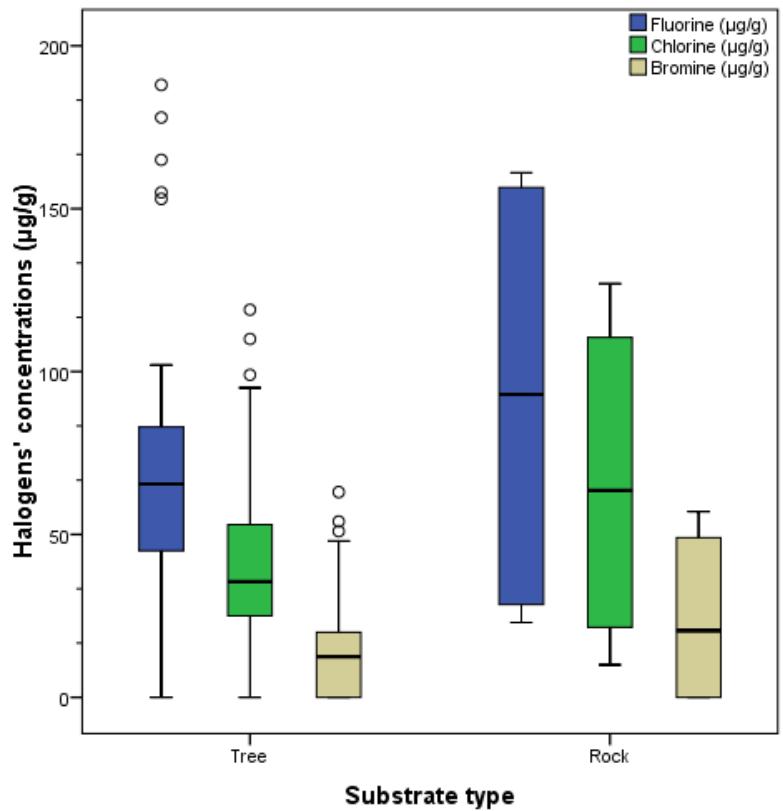 Fig. 3: Box - plot of Halogens concentrations in the substrate types Table S2 revealed that, of the eight lichen genera used for analyses, Leptogium was the most abundant, widely distributed and had very high concentrations of halogens compared to all the other species. Leptogium gelatinosum accumulating ability differs between sites. Leptogium gelatinosum samples from northern leeward flank (MC 02 from Upper Buea, MC 04 from Bomana and MC 10 and MC 11 from Ekona-Mbenge) show low accumulation of halogens over samples collected from the western windward flank Sasse (MC01 and MC03), Idenau (MC 05 and MC06), Bakingili (MC07) and Batoke (MC08 and MC09). Although, Leptogium gelatinosum recorded highest concentrations, other species like Heterodermia obscurata, Cladonia sp, Usnea articulate in BmtUM recorded high concentrations. Lichen species also showed differing accumulating potentials in substrates (Parmotrema tinctorum (MC27) a corticolous sample collected in Ekona-Mbenge accumulated more than the saxicolous specimen (MC26) collected in the same point). All the eight lichen genera showed very high concentrations of F and low levels of Br. F concentration is highest in Leptogium (188 $\mu$ g/g) and lowest in Parmotrema (0 $\mu$ g/g to 23 $\mu$ g/g). The geochemical analysis of the lichens indicated that F was the most dominant halogen (Fig. S1) with concentrations that range from 25-188 (mean = 78.00 ± 48.68 $\mu$ g/g). The range for Cl concentration was 10-127 $\mu$ g/g (mean = 47.23 ± 33.37 $\mu$ g/g), while that for Br, ranges from 0-63 $\mu$ g/g (mean = 18 ± 19.58). Fig.S2 shows that, there was highest F- bioaccumulation in Leptogium gelatinosum species in Idenau which ranges from (153 to $188~\mu \mathrm{g / g}$ ), Batoke $(165~\mu \mathrm{g / g})$, Bakingili $(178~\mu \mathrm{g / g})$, Sasse $(152$ to $155~\mu \mathrm{g / g})$ and low in Ekona-Mbenge $(34~\mu \mathrm{g / g})$. Cl bio-accumulation in the Leptogium gelatinosum species in Idenau ranges from (110 to 119 $\mu$ g/g) was highest and lowest in the Leptogium gelatinosum of Bomana (23 $\mu$ g/g), Ekona (33 $\mu$ g/g) and Hut 1 (28 $\mu$ g/g) (Fig. S3). Fig. S4, revealed no Br bio-accumulation in the Leptogium gelatinosum species in Ekona (0 $\mu$ g/g) and Bomana (0 $\mu$ g/g) but higher in Idenau (63 $\mu$ g/g). ## IV. DISCUSSION Lichens from Mt. Cameroon demonstrated significant compositional variation between species as observed on the multi-element distribution patterns even for those growing in the same area. However, specimens from the same species tend to have similar element concentration patterns. This could be explained by the fact that lichens species selectively accumulated some elements. Similarly, Rani et al. (2011) found out that, the estimated nine heavy metals in lichen samples from 12 different sites of Dehradun city by periodic monitoring and spotted Zn, Ni, Cd and Cr were higher in lichens, collected from road side while maximum quantity of Fe, Cu and Al were reported in lichens collected from central sites of the city while the lowest amounts of all the metals were reported in sites farther from city. The species Leptogium gelatinosum with very high concentrations of the halogens in all the sampling sites and even the control area of Mamfe $270~\mathrm{km}$ from Mt. Cameroon has a higher tendency to sequestrate these elements than all the other species recorded in the study. This is in accordance with the study about the suitability of the fruticose lichens Evernia prunastri, Cetraria islandica and Ramalina farinacea collected from oak trees in a remote area located in the Chianti Region (Tuscany, central Italy), as transplants for biomonitoring trace element, showed that E. prunastri has to be preferred for its higher accumulating capacity (Cercasov et al., 2002). Different lichens species in different environments have different sequestration potentials, for example, Ramalina fastigiata has been used as a bio indicator of the impact of a coal mine in Portugal Jozwiak, (2012). The very high concentrations of F in lichens in this study reflects the study of Suh et al. (2008) who measured halogen content in melt inclusions at this volcano and their results indicated an average value of $1530\mu \mathrm{g} / \mathrm{g}$ F and $1270\mu \mathrm{g} / \mathrm{g}$ Cl. They recorded unusually high F concentrations when compared to glass inclusions from Etna, Hawaii and Piton de la Fournaise. However, the Cl concentrations from Mt. Cameroon were midway between the high values measured for Etna and the low values for Hawaii and Piton de la Fournaise. These exceptionally high values relative to those recorded in this study which maybe an indication that these halogens are an important component of the volatile budget at Mt. Cameroon. These researchers reported that, the concentrations of F in olivine hosted glass inclusion from Mt. Cameroon are the highest known F concentrations for basaltic glass inclusions in the world. Altitude contributed to the halogens concentration variations as intra-species variations consistently yield high concentrations in samples collected from the downwind SW flank of the volcano. These localities lie in the path of wind bearing volcanic gas plumes from Mt. Cameroon and therefore pin their higher halogen content to passive degassing. Aiuppa et al. (2004) reported that, during explosive activity huge quantities of fluorine are deposited with ashes around the volcano up to distances of hundreds of km. Fluorine is present as an adsorbed outer layer on the tephra particles which adsorption occurs by condensation of fluoride onto the tephra particles in the plume above the volcano as it cools. The smaller tephra particles have a larger surface area, so carry more absorbed fluoride than the larger particles. The smaller particles are likely to be carried further from the volcanic source, and so their greater fluorine-carrying capacity extends the zone of potential fluorine poisoning considerably, even to regions where only a 1 mm thick deposit forms. It is advisable to sample and analyse the tephra or vegetation to identify hazardous regions. This suggests that gases emitted from the volcano are blown south-westwards and are eventually deposited close to the coast resulting in higher halogen content in the lichen species from these areas. More so, the inputs from the sea and from agricultural farms might have increased the high levels in this coastal areas. Studies by Ndlovu et al. (2019), on moss and lichen biomonitoring of atmospheric pollution in the Western Cape Province (South Africa) observed halogens to have elevated concentrations for samples collected from areas with close proximity to the ocean. That is, for both moss and lichen samples at areas closer to the ocean had higher halogen concentrations. Their results also confirmed elevated concentration levels for halogens (Cl, I, Br) in areas closest to the ocean. However, since fluorides are released into the atmosphere in large amounts by volcanic eruptions (Bajpai et al., 2011) and fluoride (F) compounds, remain in the same chemical form after they are emitted into the atmosphere, the very high levels of F bioaccumulation in this study, might have come from the degassing volcanic winds of Mt. Cameroon. Also, since other sampling points inland shows high concentration of F, degassing winds and ash deposition should have a greater influence. In this study, even though Leptogium gelatinosum was the highest bioaccmulator, Stictastenroos and Heretodemia obscurata are also good accumulators, while all the Usnea species are poor accumulators. According to Brodo et al. (2001) fruticose lichens like Usnea are very sensitive to air pollutants than foliose lichens and occur only in very pure environments. Out of different growth forms of lichens, foliose lichens are prior to metal accumulation followed by crustose and squamulose lichens (Kar et al., 2014) and least by fruticose lichens (Shukla et al., 2014). However, lichens from the Usnea species have been used to evaluate heavy metal deposition patterns in the Antarctic (Poblet et al., 2011). Certain epiphytic lichens have been particularly gained attention for their bioaccumulation potential like Hypogymnia physodes for bioaccumulation of trace elements and Pyxine cocoes for bioaccumulation of metals (Bajpai et al., 2012; Daimari et al., 2020). The differing accumulating potentials in substrates of lichen species in this study, (example, Parmotrema tinctorum (MC27) a corticolous sample collected in Ekona-Mbenge accumulated more than the saxicolous specimen (MC26) collected in the same point). Contrary, the findings of (Chettri et al., 1997), who used the lichen species Neophuscelia pulla and Xanthoparmelia tarctica to study the bioaccumulation of heavy metals in abandoned copper mines in Greece, where there was a significant correlation between the copper content in the soil(saxicolose) and that of the tree(corticolous) lichen thalli. However, it is for this reason that most studies use epiphytic macro lichens as bio-monitors for air pollutants (Loppi and Pirintsos, 2003). For example, Käffer et al. (2011) also reported corticolous lichens as environmental indicators in urban areas in southern Brazil. Furthermore, the no to slight significant difference in means of halogens concentrations with regards to substrates in this study is in accordance with the study of Bajpai et al. (2011) in Mandav city in central India illustrated that although most of the metals were absent, or present in insignificant amount in substrates, yet the thallus of lichens had significantly higher concentration of metals such as Cd, Cr, Ni and Zn. Thus it is apparent that the accumulated metals were air borne. All the eight lichen genera showed very high concentrations of F and low levels of Br. Weinstein et al. (1998) reported that, Br and I emissions are not usually of environmental importance and there is virtually no scientific literature on either element. The gas Cl is potentially very hazardous but it is very rare to be released in sufficient quantities to pose a risk (Temple et al., 1998). Chlorine concentrations of $0.4 - 2.5\mu \mathrm{g} / \mathrm{g}$ range cause severe symptoms like upper surface bleaching, epinasty (distorted growth), chlorosis (yellowing) and leaf drop to plants (Temple and Krause, 1998). The Cl/F ratio in the specimens' ranges from 0.29 to 0.94, which is lower than those measured in lichen specimens at Mt. Etna which ranges from 0.51 to 1.46 (Notcutt and Davies, 1989). According to Delmelle et al. (1997) changes in the Cl/F ratio may reflect different physico-chemical behaviour of the gases entering the atmosphere. However, Halmer et al. (2002) reported that in areas without nearby emission sources, the mean concentrations of fluoride in ambient air are generally less than $0.1\mu \mathrm{g} / \mathrm{g}$. This was observed from the control area (Mamfe 270 Km) with lower concentrations as compared to those from Mt. Cameroon. Even near emission sources, the levels of airborne fluoride usually do not exceed $2 - 3\mu \mathrm{g} / \mathrm{g}$ and in most soils, fluoride is present at concentrations ranging from 20 to $1000\mu \mathrm{g} / \mathrm{g}$. This figure can reach several thousand $\mu \mathrm{g} / \mathrm{g}$ in mineral soils with natural phosphate or fluoride deposits. Therefore, the atmospheric halogens load at Mt. Cameroon is significantly high and lichens can be potential monitors of this volcanic gas flux. ## V. CONCLUSION Leptogium gelatinosum and Heretodermia obscurata are good accumulators, while Usnea species poor accumulators and therefore can be used for pollution bio-monitoring programs in Cameroon. The Leptogium gelatinosum species is therefore a suitable species for monitoring passive degassing at Mt. Cameroon. Also, considering that, lichens of the windward flank of MC accumulated more elemental contents than those from the leeward flanks, shows that wind direction and ash fall contribute largely to pollutant load in lichen species in the windward flanks of mount Cameroon reflecting volcanic degassing as the source. This chemical analysis serves as a baseline data for future studies. ### Supplementary Information #### ACKNOWLEDGMENTS We are grateful for the support by the University of Botswana Gaborone (UBG) where the chemical analyses were performed. We thank Professor Suh Tening Aaron of the University of Buea, who is part of the interdisciplinary research framework under the theme "Understanding the environment of Mount Cameroon". We thank Dr Smith B. Babiaka of the Department of Chemistry, University of Buea, for proof reading of the manuscript. Conflict of Interests The authors declare that there is no conflict of interest whatsoever #### Funding This study did not receive any funding. #### LIST OF TABLES Table S1: Lichen species code, sites and names used for chemical analysis. <table><tr><td>Chemical Code</td><td>Site</td><td>Species name</td><td>Chemical Code</td><td>Site</td><td>Species name</td></tr><tr><td>MC 01</td><td>BmtSas</td><td>Leptogium gelatinosum</td><td>MC 18</td><td>BmtBok</td><td>Sticta stenroos</td></tr><tr><td>MC 02</td><td>Bmt UM</td><td>Leptogium gelatinosum</td><td>MC 19</td><td>BmtUM</td><td>Cladonia sp</td></tr><tr><td>MC 03</td><td>BmtSas</td><td>Leptogium gelatinosum</td><td>MC 20</td><td>BmtUM</td><td>Usnea articulata</td></tr><tr><td>MC 04</td><td>Boma</td><td>Leptogium gelatinosum</td><td>MC 21</td><td>BmtUM</td><td>Usnea articulata</td></tr><tr><td>MC 05</td><td>Iden</td><td>Leptogium gelatinosum</td><td>MC 22</td><td>BmtUM</td><td>Usnea articulata</td></tr><tr><td>MC 06</td><td>Iden</td><td>Leptogium gelatinosum</td><td>MC 23</td><td>BmtUM</td><td>Usnea florida</td></tr><tr><td>MC 07</td><td>Bakin</td><td>Leptogium gelatinosum</td><td>MC 24</td><td>BmtSop</td><td>Canoparmelia concrescens</td></tr><tr><td>MC 08</td><td>Batok</td><td>Leptogium gelatinosum</td><td>MC 25</td><td>EkLav</td><td>Parmotrema tinctorum</td></tr><tr><td>MC09</td><td>Batok</td><td>Leptogium gelatinosum</td><td>MC 26</td><td>EkLav</td><td>Parmotrema tinctorum</td></tr><tr><td>MC 10</td><td>EkLav</td><td>Leptogium gelatinosum</td><td>MC27</td><td>EkLav</td><td>Parmotrema tinctorum</td></tr><tr><td>MC 11</td><td>EkLav</td><td>Leptogium gelatinosum</td><td>MC 28</td><td>EkIrad</td><td>Parmotrema tinctorum</td></tr><tr><td>MC 12</td><td>Mamfe</td><td>Leptogium gelatinosum</td><td>MC 29</td><td>EkLav</td><td>Flavoparmelia caperata</td></tr><tr><td>MC 13</td><td>BmtUM</td><td>Parmotrema tinctorum</td><td>MC 30</td><td>EkIrad</td><td>Flavoparmelia caperata</td></tr><tr><td>MC 14</td><td>BmtUB</td><td>Parmotrema tinctorum</td><td>MC 31</td><td>EkLav</td><td>Heterodermia obscurata</td></tr><tr><td>MC 15</td><td>BmtUM</td><td>Flavoparmelia caperata</td><td>MC 32</td><td>EkLav</td><td>Heterodermia obscurata</td></tr><tr><td>MC 16</td><td>BmtUB</td><td>Flavoparmelia caperata</td><td>MC 33</td><td>EkLav</td><td>Usnea dasypoga</td></tr><tr><td>MC 17</td><td>BmtUM</td><td>Heterodermia obscurata</td><td>MC34</td><td>Boman</td><td>Heterodermia japonica</td></tr></table> Table S2: Concentration of halogens analyzed for in lichen samples from MC(μg/g). <table><tr><td>Chemical Code</td><td>Site</td><td>Species name</td><td>Substrate type</td><td>F</td><td>Cl</td><td>Br</td></tr><tr><td>MC 01</td><td>BmtSas</td><td>Leptogium gelatinosum</td><td>Tree</td><td>155</td><td>89</td><td>48</td></tr><tr><td>MC 02</td><td>Bmt UM</td><td>Leptogium gelatinosum</td><td>Tree</td><td>58</td><td>28</td><td>13</td></tr><tr><td>MC 03</td><td>BmtSas</td><td>Leptogium gelatinosum</td><td>Rock</td><td>152</td><td>94</td><td>57</td></tr><tr><td>MC 04</td><td>Boma</td><td>Leptogium gelatinosum</td><td>Tree</td><td>55</td><td>23</td><td>0</td></tr><tr><td>MC 05</td><td>Iden</td><td>Leptogium gelatinosum</td><td>Tree</td><td>188</td><td>110</td><td>54</td></tr><tr><td>MC 06</td><td>Iden</td><td>Leptogium gelatinosum</td><td>Tree</td><td>153</td><td>119</td><td>63</td></tr><tr><td>MC 07</td><td>Bakin</td><td>Leptogium gelatinosum</td><td>Tree</td><td>165</td><td>99</td><td>45</td></tr><tr><td>MC 08</td><td>Batok</td><td>Leptogium gelatinosum</td><td>Tree</td><td>178</td><td>87</td><td>51</td></tr><tr><td>MC09</td><td>Batok</td><td>Leptogium gelatinosum</td><td>Rock</td><td>161</td><td>127</td><td>41</td></tr><tr><td>MC 10</td><td>EkLav</td><td>Leptogium gelatinosum</td><td>Tree</td><td>42</td><td>23</td><td>0</td></tr><tr><td>MC 11</td><td>EkLav</td><td>Leptogium gelatinosum</td><td>Rock</td><td>34</td><td>33</td><td>0</td></tr><tr><td>MC 12</td><td>Mamfe</td><td>Leptogium gelatinosum</td><td>Tree</td><td>25</td><td>0</td><td>0</td></tr><tr><td>MC 13</td><td>BmtUM</td><td>Parmotrema tinctorum</td><td>Tree</td><td>55</td><td>39</td><td>12</td></tr><tr><td>MC 14</td><td>BmtUB</td><td>Parmotrema tinctorum</td><td>Tree</td><td>43</td><td>27</td><td>0</td></tr><tr><td>MC 15</td><td>BmtUM</td><td>Flavoparmelina caperata</td><td>Tree</td><td>55</td><td>41</td><td>0</td></tr><tr><td>MC 16</td><td>BmtUM</td><td>Flavoparmelina caperata</td><td>Tree</td><td>67</td><td>23</td><td>11</td></tr><tr><td>MC 17</td><td>BmtUM</td><td>Heterodermia obscurata</td><td>Tree</td><td>83</td><td>46</td><td>12</td></tr><tr><td>MC 18</td><td>BmtBok</td><td>Stictastenroos</td><td>Tree</td><td>60</td><td>34</td><td>19</td></tr><tr><td>MC 19</td><td>BmtUM</td><td>Cladonia sp</td><td>Tree</td><td>102</td><td>95</td><td>34</td></tr><tr><td>MC 20</td><td>BmtUM</td><td>Usnea articulate</td><td>Tree</td><td>64</td><td>42</td><td>13</td></tr><tr><td>MC 21</td><td>BmtUM</td><td>Usnea articulate</td><td>Tree</td><td>39</td><td>38</td><td>0</td></tr><tr><td>MC 22</td><td>BmtUM</td><td>Usnea articulate</td><td>Tree</td><td>77</td><td>53</td><td>0</td></tr><tr><td>MC 23</td><td>BmtUM</td><td>Usne aflorida</td><td>Tree</td><td>69</td><td>37</td><td>15</td></tr><tr><td>MC 24</td><td>BmtSop</td><td>Canoparmelia concrescens</td><td>Tree</td><td>43</td><td>31</td><td>0</td></tr><tr><td>MC 25</td><td>EkLav</td><td>Parmotrema tinctorum</td><td>Tree</td><td>0</td><td>0</td><td>0</td></tr><tr><td>MC 26</td><td>EkLav</td><td>Parmotrema tinctorum</td><td>Rock</td><td>23</td><td>10</td><td>0</td></tr><tr><td>MC27</td><td>EkLav</td><td>Parmotrema tinctorum</td><td>Tree</td><td>67</td><td>32</td><td>15</td></tr><tr><td>MC 28</td><td>EkIrad</td><td>Parmotrema tinctorum</td><td>Tree</td><td>45</td><td>31</td><td>18</td></tr><tr><td>MC 29</td><td>EkLav</td><td>Flavoparmelina caperata</td><td>Tree</td><td>78</td><td>23</td><td>0</td></tr><tr><td>MC 30</td><td>EkIrad</td><td>Flavoparmelina caperata</td><td>Tree</td><td>67</td><td>41</td><td>0</td></tr><tr><td>MC 31</td><td>EkLav</td><td>Heterodermia obscurata</td><td>Tree</td><td>90</td><td>58</td><td>20</td></tr><tr><td>MC 32</td><td>EkLav</td><td>Heterodermia obscurata</td><td>Tree</td><td>77</td><td>34</td><td>13</td></tr><tr><td>MC 33</td><td>EkLav</td><td>Usnea dasypoga</td><td>Tree</td><td>45</td><td>24</td><td>27</td></tr><tr><td>MC34</td><td>Boma</td><td>Heterodermia japonica</td><td>Tree</td><td>34</td><td>25</td><td>10</td></tr><tr><td>Mean</td><td></td><td></td><td></td><td>78</td><td>47</td><td>18</td></tr><tr><td>Min</td><td></td><td></td><td></td><td>0</td><td>0</td><td>0</td></tr><tr><td>Max</td><td></td><td></td><td></td><td>188</td><td>127</td><td>63</td></tr><tr><td>SD</td><td></td><td></td><td></td><td>49</td><td>33</td><td>20</td></tr></table>

Generating HTML Viewer...

References

61 Cites in Article
S Ahmad,M Daud,I Qureshi (2007). Use of bio-monitors to assess the atmospheric changes.
A Aiuppa,S Bellomo,W D'alessandro,C Federico,M Ferm,M Valenza (2004). Volcanic plume monitoring at Mount Etna by diffusive (passive) sampling.
S Ayrault,R Clochiatti,F Carrot,L Daudin,J Bennett (2007). Factors to consider for trace element deposition biomonitoring surveys with lichen transplants.
Rajesh Bajpai,D Upreti,S Dwivedi,S Nayaka (2011). Lichen as quantitative biomonitors of atmospheric heavy metals deposition in Central India.
Rajesh Bajpai,D Upreti (2012). Accumulation and toxic effect of arsenic and other heavy metals in a contaminated area of West Bengal, India, in the lichen Pyxine cocoes (Sw.) Nyl..
R Bargagli (2016). Moss and Lichen Biomonitoring of Atmospheric Mercury: A Review.
J Bennett (2006). Lichens and air pollution.
Jarle Bjerke,Tina Werner Dahl (2002). Distribution patterns of usnic acid-producing lichens along local radiation gradients in West Greenland.
Lenka Brodeková,Alan Gilmer,Paul Dowding,Howard Fox,Anna Guttová (2006). An Assessment of Epiphytic Lichen Diversity and Environmental Quality in Knocksink Wood Nature Reserve, Ireland.
I Brodo,S Sharnoff,S Sharnoff (2001). Lichens of North America.
Jie Chen,Hans-Peter Blume,Lothar Beyer (2000). Weathering of rocks induced by lichen colonization — a review.
M Chettri,T Sawidis,S Karataglis (1997). Lichens as a tool for biogeochemical prospecting.
Marcelo Conti,Raquel Jasan,Maria Finoia,Ivo Iavicoli,Rita Plá (2016). Trace elements deposition in the Tierra del Fuego region (south Patagonia) by using lichen transplants after the Puyehue-Cordón Caulle (north Patagonia) volcanic eruption in 2011.
Shane Cronin,Donald Sharp (2002). Environmental impacts on health from continuous volcanic activity at Yasur (Tanna) and Ambrym, Vanuatu.
Chicita Culberson,William Culberson (2001). Future Directions in Lichen Chemistry.
R Daimari (2020). Biomonitoring by epiphytic lichen species Pyxine cocoes (Sw.) Nyl.: Understanding characteristics of trace metal in ambient air of different land uses in mid-Brahmaputra Valley.
M Delancey,D Mark (2000). Historical Dictionary of the Republic of Cameroon.
Bernard Déruelle,Jean N'ni,Robert Kambou (1997). Mount Cameroon: an active volcano of the Cameroon Line.
Sananda Dey,Biplab Giri (2015). Fluoride Fact on Human Health and Health Problems: A Review.
P Diana,V Patrícia,R Armindo Dos Santos (2019). Unknown Title.
Neil Donahue (2018). Air Pollution and Air Quality.
María García,Laura Borgnino (2015). CHAPTER 1. Fluoride in the Context of the Environment.
Jacob Garty,Tal Levin,Yehudit Cohen,Haya Lehr (2002). Biomonitoring air pollution with the desert lichen <i>Ramalina maciformis</i>.
R Godinho,H Wolterbeek,T Verburg,M Freitas (2008). Bioaccumulation behaviour of transplants of the lichen Flavoparmelia caperata in relation to total deposition at a polluted location in Portugal.
A Golubev,V Golubeva,N Krylov,V Kuznetsova,S Mavrin,А Aleinikov,W Hoppes,K Surano (2006). On monitoring anthropogenic airborne uranium concentrations and 235U/238U isotopic ratio by Lichen – bio-indicator technique.
M Grasso,R Clocchiatti,F Carrot,C Deschamps,F Vurro (1999). Lichens as bioindicators in volcanic areas: Mt. Etna and Vulcano Island (Italy).
Markus Hauck (2005). Epiphytic lichen diversity on dead and dying conifers under different levels of atmospheric pollution.
Darren Hess,Dana Coker,Jeannette Loutsch,Jon Russ (2008). Production of oxalates <i>In Vitro</i> by Microbes Isolated from Rock Surfaces with prehistoric paints in the Lower Pecos Region, Texas.
K Jatinder,K Roshni,R Himanshu,D Upreti,A Tayade,S Hota,O Chaurasia,R Srivastava (2012). Diversity of lichens along altitudinal and land use gradients in the Trans Himalayan cold desert of Ladakh.
S Jitka,N Tomás,R Jan,M Martin,K Petra,Petra Ludek (2010). The characteristics of rare earth elements in bulk precipitation, through fall, foliage and lichens in the Lesní potok catchment and its vicinity, Czech Republic.
S Jovans (2008). Lichen bioindication of biodiversity, air quality, and climate: baseline results from monitoring in Washington, Oregon, and California..
Márcia Käffer,Suzana Martins,Camila Alves,Viviane Pereira,Jandyra Fachel,Vera Vargas (2011). Corticolous lichens as environmental indicators in urban areas in southern Brazil.
S Kar,A Samal,J Maity,S Santra (2014). Diversity of epiphytic lichens and their role in sequestration of atmospheric metals.
M Jóźwiak (2012). Macroscopic changes of Hypogymnia physodes (L.) Nyl. in antropogenic stress conditions.
R Larsen,J Bell,P James,P Chimonides,F Rumsey,A Tremper,O Purvis (2007). Lichen and bryophyte distribution on oak in London in relation to air pollution and bark acidity.
James Lawrey (1986). Biological Role of Lichen Substances.
Diana Linhares,Patrícia Garcia,Leslie Amaral,Teresa Ferreira,Armindo Dos Santos Rodrigues (2017). Safety Evaluation of Fluoride Content in Tea Infusions Consumed in the Azores—a Volcanic Region with Water Springs naturally Enriched in Fluoride.
E Llop,P Pinho,P Matos,M Pereira,C Branquinho (2012). The use of lichen functional group asindicators of air quality in a mediterranean urban environment.
S Loppi,S Pirintsos (2003). Epiphytic lichens as sentinels for heavy metal pollution at forest ecosystems (central Italy).
G Lorenzini,C Grassi,C Nali,A Petiti,S Loppi,L Tognotti (2006). Leaves of Pittosporum tobira as indicators of airborne trace element and PM10 distribution in central Italy.
J Monge-Nájera,I María,R Marta,V Méndez (2002). A new method to assess air pollution using lichens as bio-indicators.
J Morris,W Purvis (2007). Lichens (Life).
S Munzi,L Paoli,E Fiorini,S Loppi (2012). Physiological response of the epiphytic lichen Evernia prunastri (L.) Ach. to ecologically relevant nitrogen concentrations.
N Ndlovu,M Frontasyeva,R Newman,P Maleka (2019). Moss and Lichen Biomonitoring of Atmospheric Pollution in the Western Cape Province (South Africa).
Peter Nelson,Tim B Wheeler (2016). Persistence of epiphytic lichens along a tephra-depth gradient produced by the 2011 Puyehue-Cordón Caulle eruption in Parque Nacional Puyehue, Chile.
Geoff Notcutt,Frances Davies (1989). Accumulation of volcanogenic fluoride by vegetation: Mt. Etna, sicily.
P Pinho,A Bergamini,P Carvalho,C Branquinho,S Stofer,C Scheidegger,C Máguas (2012). Lichen functional groups as ecological indicators of the effects of land-use in Mediterranean ecosystems.
A Poblet,S Andrade,M Scagliola,C Vodopivez,A Curtosi,A Pucci,J Marcovecchio (1997). The use of epilithic Antarctic lichens (Usnea aurantiacoatra and U. antartica) to determine deposition patterns of heavy metals in the Shetland Islands, Antarctica.
Manju Rani,Vertika Shukla,D Upreti,G Rajwar (2011). Periodical monitoring with lichen, Phaeophyscia hispidula (Ach.) Moberg in Dehradun city, Uttarakhand, India.
Florian Schwandner,Terry Seward,Andrew Gize,P Hall,Volker Dietrich (2004). Diffuse emission of organic trace gases from the flank and crater of a quiescent active volcano (Vulcano, Aeolian Islands, Italy).
Vertika Shukla,Upreti D.K.,Rajesh Bajpai (2014). Lichens to Biomonitor the Environment.
B Smodis (2007). Investigation of trace element atmospheric pollution by nuclear analytical techniques at a global scale: Harmonised approaches supported by the IAEA.
K Srivastava,P Bhattacharya,H Rai,P Nag,R Gupta (2015). Epiphytic lichen ramalina as indicator of atmospheric metal deposition, along land use gradients in and around binsar Wildlife Sanctuary.
L Stefano,F Luisa (2006). Lichen Diversity and Lichen Transplants as Monitors of Air Pollution in a Rural Area of Central Italy.
C Suh,J Luhr,M Njome (2008). Olivine-hosted glass inclusions from Scoriae erupted in 1954–2000 at Mount Cameroon volcano, West Africa.
C Suh,R Sparks,J Fitton,S Ayonghe,C Annen,R Nana,A Luckman (2003). The 1999 and 2000 eruptions of Mount Cameroon: eruption behaviour and petrochemistry of lava.
P Temple,J Sun,G Krause (1998). Peroxyacetyl nitrates (PAN) and other minor pollutants.
C Van Herk,A Aptroot,H Van Dobben (2002). Long-term monitoring in the Netherlands suggests that lichens respond to global warming.
T Walker,P Crittenden,S Young (2003). Regional variation in the chemical composition of winter snow pack and terricolous lichens in relation to sources of acid emissions in the Usa river basin, northeast European Russia.
L Weinstein,A Davison,U Arndt (1998). Fluoride. In Recognition of Air Pollutant Injury to Vegetation: A Pictorial Atlas.
No ethics committee approval was required for this article type.
Data Availability
Not applicable for this article.
How to Cite This Article
Ayuk Elizabeth Orock. 2026. \u201cLichen Species as Bio-accumulator of some Halogens on Mount Cameroon Valcano, West Africa\u201d. Global Journal of Human-Social Science - B: Geography, Environmental Science & Disaster Management GJHSS-B Volume 22 (GJHSS Volume 22 Issue B4).
Explore published articles in an immersive Augmented Reality environment. Our platform converts research papers into interactive 3D books, allowing readers to view and interact with content using AR and VR compatible devices.
Your published article is automatically converted into a realistic 3D book. Flip through pages and read research papers in a more engaging and interactive format.
Our website is actively being updated, and changes may occur frequently. Please clear your browser cache if needed. For feedback or error reporting, please email [email protected]
Thank you for connecting with us. We will respond to you shortly.