In this paper, the mathematical analysis is carried out from many angles, so that the theoretical calculation problem of the circular metal wall cut-off waveguide used as a premary attenuation standard is completely solved, and the Chinese national standard of the attenuation quantity is established. The benchmark was completed by the Chinese National Institute of Metrology (NIM) with an accuracy of 5×10 -5 ; Reach the international advanced level. The calculation accuracy provided in this paper is 10 -6 ~10 -7 . This is a good example of a project combining theory and practice.
## I. INTRODUCTION
In microwave measurement technology, the parameters to be measured are frequency, power, impedance, attenuation, phase shift, etc., and attenuation measurement occupies a prominent position[1]. Microwave attenuation measurement methods, an important method is the replacement method, including high frequency replacement method (microwave replacement method), medium frequency replacement method, low frequency replacement method (audio replacement method), the essence is to compare the unknown attenuation with the known precise value, so as to measure the value of the unknown attenuation. Therefore, a high precision standard attenuator is required. The attenuator of WBCO (cut-off waveguide attenuator) is commonly used for IF substitution[2]. Because the receiving electrode is usually a mobile structure (mounted on a piston), it is also called piston attenuator[3]. In addition, because of its highest accuracy, it can be used as a national measurement standard, also known as the primary standard of attenuation.
It must be pointed out that the accuracy of the microwave attenuation measurement system is lower than that of the cutoff attenuator used as the standard; For example, if the accuracy of the latter is $5 \times 10^{-5}$, the former is $10^{-3} \sim 10^{-4}$. In China, the microwave attenuation measurement system produced by microwave instrument factories in the 1980s had an error of no more than one thousandth. Of course, the accuracy of $5 \times 10^{-5}$ standard attenuator is difficult to do, but in 1980 by the Chinese Academy of Metrology (NIM) research group completed the project reached this level, known as the first attenuation standard or National attenuation basic standard. Below this is the Secondary attenuation standard, its standard cut-off attenuator accuracy is $5 \times 10^{-4}$, then the accuracy of the entire microwave attenuation measurement system is $10^{-3}$, that is, the error is not more than one thousandth.
From 1966 to 1980, the American Bureau of Standards (NBS), the National Institute of Physics Laboratory (NPL), and NIM all built a first-stage attenuator working in the medium frequency (30MHz), all using a cut-off waveguide attenuator. Professor Mengzong Song of NIM is the chief designer, and engineers Yongjian Xia and Ronggen Mo are responsible for the structural design[4]. The machining problem of precision circular waveguide is solved[5]. Zhi-xun Huang is responsible for theoretical calculation and error analysis[6]. In addition, there are other researchers involved in this project, after several years of efforts finally successful, technical indicators reached the international advanced level. This paper is a comprehensive theoretical summary by the author, including my new equations, which are contributions to the basic waveguide theory.
## II. STANDARD ATTENUATORS IN MICROWAVE ATTENUATION MEASUREMENT
The working principle of the cutoff waveguide attenuator is the exponential decline characteristic of the evanescent field in the waveguide when the waveguide cutoff point is below $(\mathbf{f} < \mathbf{f}_{\mathrm{c}}, \lambda > \lambda_{\mathrm{c}})$, and a circular waveguide is placed along the direction $z$:
$$
E = E _ {0} \mathrm {e} ^ {- \alpha z}
$$
The field strength at $z = 0$ (starting point) is $\mathbf{E}_0$. If $z = l$, the field strength is $\mathbf{E}_1$, there is:
$$
E_{l}=E_{0}\mathrm{e}^{-\alpha l}
$$
If the attenuation generated by a waveguide of length $l$ is defined as $\mathbf{A}$, then there is
$$
A = \ln \frac{E_{0}}{E_{l}} = \alpha l \, (\mathrm{Np})
$$
For example, when $A = 20 \mathrm{~dB} = 2.3 \mathrm{~Np}$, $e^{-A} = 0.1$. This means that when the design is $\alpha = 1 \mathrm{~dB} / \mathrm{mm}$, the field strength decreases to 1/10 of the starting value after only 20 mm along the direction $z$. This is a fast rate of descent, indicating that large attenuation, such as more than 100 dB, can be obtained only with a shorter cut-off waveguide.
When the electromagnetic wave propagates in the metal wall waveguide, there will be a cutoff phenomenon, that is, only the frequency $\mathbf{f} > \mathbf{f}_{\mathrm{c}}$ wave, above the cutoff frequency, can propagate. At the frequency of $\mathbf{f} < \mathbf{f}_{\mathrm{c}}$, the evanescent field is characteristic, which is a reactive energy storage field. Such devices, known as cut-off waveguides (WBCO), have prominent uses in electronic instrument design. In 1942, E. Linder[7] gave a formula for calculating the attenuation constant of the cutoff waveguide:
$$
\alpha = \frac{2\pi}{\lambda_{c}} \sqrt{1 - \left(\frac{\lambda_{c}}{\lambda}\right)^{2}} \tag{3}
$$
The cut-off wavelength $\lambda_{\mathrm{c}}$ is determined by the size of the waveguide cross section. We know that length and time are the two basic units of metrology; It is now associated with two basic units, which determines that it can obtain $\alpha$ high accuracy (if the waveguide machining size is very precise). Of course, Linder's formula is not very accurate, so improving the formula is a work for future generations. Both R. Grranthan[8] in 1948 and R. Rauskolb[9] in 1962 made efforts, but the accuracy of their formulas was not high enough to meet the requirements for the design and construction of first-order standard attenuators. The problem was solved by me.
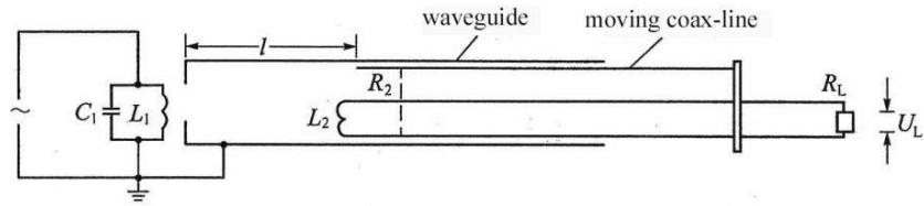 Figure 1: Example of Output Attenuator for a Meter Wave Standard Signal Generator
To visualize the actual operating state of the cut-off waveguide, Figure 1 shows the output circuit of a standard signal generator capable of obtaining a voltage output in the microvolt $(\mu V)$ range[3]. When the receiving electrode (L) mounted on the coaxial line is moved, the output voltage U is uniformly and continuously changed for use by the experimenter. Here, $l$ represents the length of the actual operating cut-off waveguide.
The main mode of the circular waveguide, strictly written as $\mathrm{HE}_{11}$ mode, indicates that the effect of the finite conductivity of the wall cannot be ignored, and the $H_{11}$ mode ( $T E_{11}$ mode) under ideal conditions will be slightly affected by the mode coupling[4]. But generally speaking, the main mode in the circular waveguide is $H_{11}$ mode ( $T E_{11}$ mode); If its inner diameter is $2\mathbf{a}$, the cutoff wavelength of the mode is
$$
\lambda_{\mathrm{c.11}} = \frac{2\pi}{k} a = 3.412 a\tag{4}
$$
Set $\lambda$ to the operating wavelength (depending on the signal source), so in order to obtain the $H_{11}$ -mode evanescent field must be satisfied:
$$
a < \frac {\lambda}{3 . 4 1 2} \tag {5}
$$
Here are the transverse dimensions of the circular waveguide used in the primary attenuation standards built by the highest metrological institutions in several countries: $2a = 3.2\mathrm{cm}$ (NIM); $2a \approx 5.06\mathrm{cm}(\mathrm{NPL})$; $2a \approx 8.12\mathrm{cm}(\mathrm{NBS})$.
The relation A-1 equation of the cutoff attenuator is not linear at all locations and has A nonlinear segment at smaller 1 (and therefore smaller $\mathbf{A}$ ) $^{[3]}$. In order to maintain high accuracy, the application can avoid this section, that is, avoid the initial attenuation section of about 20dB, that is, maintain the linear relationship $\mathbf{A} = \alpha \mathbf{1}$. The laser length measurement technology can be accurately measured, so the focus of the study turns to the attenuation constant $\alpha$. It must be pointed out that the outstanding contribution of the author is the monograph «Introduction to the Theory of Waveguide Cutoff Below», published in 1991, which makes the cutoff waveguide theory into a complete system, and derives some new equations and formulas, and gives the solution methods[10]. In the book, it is pointed out that for microwave attenuation measurement, a branch of metrology, in the 30 years from 1950 to 1980, the accuracy of the cutoff attenuator standard was increased from $5 \times 10^{-3}$ to close to $5 \times 10^{-5}$, because it is basically a calculation standard, and the attenuation constant is mainly determined by the basic unit (length and frequency). In the case of the increasing level of machining and surface treatment technology, it is required to theoretically derive the attenuation constant formula with higher accuracy (higher than $5 \times 10^{-5}$ ). For the $\mathrm{HE}_{11}$ mode in the metal-walled circular waveguide, the formula is derived as[4]:
$$
\alpha_{11} = \frac{2\pi}{\lambda_c} \sqrt{ \frac{1}{2} \left[ 1 - \left(\frac{\lambda_c}{\lambda}\right)^2 \varepsilon_r - \mathbf{J}_{11} \right] + \frac{1}{2} \sqrt{ \left[ 1 - \left(\frac{\lambda_c}{\lambda}\right)^2 \varepsilon_r - \mathbf{J}_{11} \right]^2 + \mathbf{J}_{11}^2 } } \quad (\mathrm{Np}/\mathrm{m}) \tag{6}
$$
among
$$
\mathrm{J}_{11} = \frac{g\tau}{a} = \mu_{\mathrm{rc}} \left[ 1 + \frac{1}{k_{11}^{2} - 1} \left(\frac{\lambda_{c}}{\lambda}\right)^{2} \right] \frac{\tau}{a} \tag{7}
$$
Where $\mu_{\mathrm{rc}}$ is the relative magnetic permeability of the wall metal; $\varepsilon_{\mathrm{r}}$ is the relative dielectric constant of the filling medium; $\tau$ is the skin depth of the inner wall, $\tau = (\pi \mu \sigma f)^{-1/2}$, where $\sigma$ is the RF conductivity of the wall metal, $\mu = \mu_{\mathrm{rc}} \mu_0$ is the magnetic permeability of the wall metal. The calculation shows that the formula derived by the author is the most accurate one of the same kind (the accuracy is $1 \times 10^{-6}$ ), which can meet the calculation needs of establishing high precision national attenuation standard.
It can be obtained from formula (2):
$$
\mathrm{d}A = \frac{\mathrm{d}\alpha}{\alpha} A + \alpha \cdot \mathrm{d}l \tag{8}
$$
The above formula indicates the method of giving electrical performance indicators for standard cutoff attenuators, which is very important. The first term on the right side of the equation is caused by the circular cut-off waveguide, and the second term is caused by the length measuring (displacement measuring) mechanism. Since the 1970s, due to the development of laser length measurement technology, the second item has been greatly reduced (such as displacement resolution up to 0.0001dB), so the main task is to reduce $\mathbf{d}\alpha / \alpha$. The basic parameters of the first order cutoff attenuation standard developed successfully by various countries are derived from two main factors: the uncertainty of the radius of the circular waveguide (da/a) and the uncertainty of the RF conductivity of the waveguide wall material ( $\mathbf{d}\sigma / \sigma$ ). The operating mode is $\mathrm{H}_{11}(\mathrm{TE}_{11})$, and the operating frequency is $30\mathrm{MHz}$.
Now look at where the US and China have reached. According to literature [11], the NBS of the United States in 1960 was as follows: the average inner diameter of the cut-off waveguide was $81.21015\mathrm{mm}$ (at $20^{\circ}\mathrm{C}$ ), the diameter machining uniformity was $\pm 0.762\mu \mathrm{m}$, the diameter measurement uncertainty was $\pm 1.27\mathrm{mm}$, the radio frequency conductivity of the tube wall was $1.2825\times 10^{-7}(\Omega \cdot \mathrm{m})^{-1}$, and the uncertainty was $\mathbf{d}\sigma / \sigma = \pm 5\%$. For such a waveguide, the attenuation constant $\alpha = 0.393701$ dB/mm(at $20^{\circ}\mathrm{C}$ ). The partial error and the uncertainty of pipe diameter caused by $\pm 3\times 10^{-5}$, the small change of temperature in the constant temperature room caused by $\pm 1\times 10^{-5}$, and the uncertainty of pipe wall conductivity caused by $\pm 2.6\times 10^{-5}$. NBS technical report gives $\alpha = 0.393701$ dB/mm. $\mathbf{d}\alpha / \alpha = \pm 1\times 10^{-4}$, that is, one part in 10,000.
In addition, according to literature [4], the situation of NIM in China in 1980 was as follows: average inner diameter of cutoff waveguide $31.96254\mathrm{mm}$ (at $20^{\circ}\mathrm{C}$ ), non-uniformity of pipe diameter processing $\pm 0.5\mu \mathrm{m}$, uncertainty of pipe diameter measurement $\pm 0.6\mu \mathrm{m}$, radio frequency conductivity of pipe wall $= 1.6034\times 10^{-7}(\Omega \cdot \mathrm{m})^{-1}$, uncertainty $\pm 4\%$. In this case, the attenuation constant $\alpha = 0.99995775$ dB/mm ( $20^{\circ}\mathrm{C}$ ); After synthesizing the partial errors, the NIM technical report gives $\mathrm{d}\alpha /\alpha = 5\times 10^{-5}$, that is, 5 parts per 100,000.
It can be seen that the attenuation standard established by China's NIM is better than that established by the NBS of US. As for a lot of theoretical analysis work is not NBS.
## III. HISTORICAL BACKGROUND: FROM THOMSON EQUATION TO CMS EQUATION
British scientist Joseph Thomson (1856-1940) won the Nobel Prize in Physics in 1906 for his discovery of the electron. In 1893 J. Thomson published a book: Notes on New Research in Electromagnetics - a continuation of Professor Clerk Maxwell's «Treatises on Electricity and Magnetism» [12]. It fully affirms the realizability of transmitting electromagnetic waves in a circular metal-walled tube (that is, a circular waveguide). Why is Thomson so early can come to the right conclusion? This is mainly because his mathematical starting point is correct: first analyze the electrical vibration of the cylindrical cavity inside the conductor, that is, solve the two-dimensional wave equation. This made him the first scientist in history to predict waveguides.

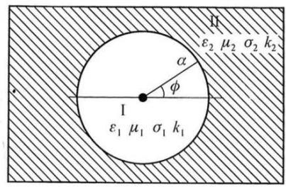
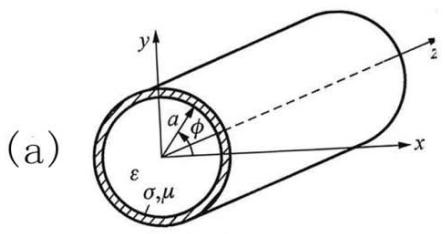
(b) Figure 2: Circular Waveguide For the reader's ease of understanding, Thomson's analysis is presented in today's notation, and its system of units is changed to SI. A medium cylinder with radius of (a) is buried in a uniform infinite conductor space $(\varepsilon_{\mathrm{c}}, \mu_{\mathrm{c}})$, and the cylindrical coordinate system $(r, \phi, z)$ is taken for analysis (FIG. 2). Thomson showed that the following partial differential equations held in the medium:
$$
\frac{\partial^{2}H_{z}}{\partial x^{2}} + \frac{\partial^{2}H_{z}}{\partial y^{2}} = \frac{1}{V^{2}} \frac{\partial^{2}H_{z}}{\partial t^{2}}
$$
He called V "the speed of electrodynamic action" propagating through a medium, which is actually the speed of electromagnetic waves. The following partial differential equation holds in the conductor:
$$
\frac {\partial^ {2} H _ {z}}{\partial x ^ {2}} + \frac {\partial^ {2} H _ {z}}{\partial y ^ {2}} = \sigma \mu_ {\mathrm {c}} \frac {\partial^ {2} H _ {z}}{\partial t}
$$
Where $\sigma$ is electrical conductivity. The above two formulas can be written as
$$
\nabla_ {t} ^ {2} H _ {z} = \frac {1}{V ^ {2}} \frac {\partial^ {2} H _ {z}}{\partial t ^ {2}} \quad (i n m e d i u m)
$$
$$
\nabla_ {t} ^ {2} H _ {z} = \sigma \mu_ {\mathrm{c}} \frac{\partial^ {2} H _ {z}}{\partial t} (in conductor)
$$
This was Thomson's starting point. When you take a cylindrical coordinate system, then
$$
\frac{\partial^ {2} H _ {z}}{\partial r ^ {2}} + \frac{1}{r} \frac{\partial^ {2} H _ {z}}{\partial r} + \frac{1}{r ^ {2}} \frac{\partial^ {2} H _ {z}}{\partial \phi^ {2}} = \frac{1}{V ^ {2}} \frac{\partial^ {2} H _ {z}}{\partial t ^ {2}} \quad \text{(inmedium)}
$$
$$
\frac{\partial^ {2} H _ {z}}{\partial r ^ {2}} + \frac{1}{r} \frac{\partial^ {2} H _ {z}}{\partial r} + \frac{1}{r ^ {2}} \frac{\partial^ {2} H _ {z}}{\partial \phi^ {2}} = \sigma \mu_ {\mathrm{c}} \frac{\partial^ {2} H _ {z}}{\partial t} \quad (\text{inside})
$$
Thomson assumed $\mathbf{H}_{\mathrm{z}}$ changes according to the law of $\cos \phi \cdot \mathrm{e}^{\mathrm{j}\omega t}$, which in fact introduced the steady state, monochromatic simple harmonic concept proposed by Helmholtz (1821-1894) in 1860. In this way, two ordinary differential equations are obtained:
$$
\frac{\mathrm{d} ^ {2} H _ {z}}{\mathrm{d} r ^ {2}} + \frac{1}{r} \frac{\mathrm{d} H _ {z}}{\mathrm{d} r} + \left(\frac{\omega^ {2}}{V ^ {2}} - \frac{m ^ {2}}{r ^ {2}}\right) H _ {z} = 0 \quad (\text{inmedium}) \tag{9}
$$
$$
\frac{\mathrm{d} ^ {2} H _ {z}}{\mathrm{d} r ^ {2}} + \frac{1}{r} \frac{\mathrm{d} H _ {z}}{\mathrm{d} r} - \left(j \omega \sigma \mu_ {\mathrm{c}} + \frac{m ^ {2}}{r ^ {2}}\right) H _ {\neq 0} (\text{inconductor})
$$
Where $m$ is a positive integer. Let $\gamma_{\mathrm{c}} = \sqrt{\mathrm{j}\omega\mu_{\mathrm{c}}\sigma}$, then the equation in the conductor is
$$
\frac{\mathrm{d}^{2}H_{z}}{\mathrm{d}\left(\gamma_{\mathrm{c}}r\right)^{2}} + \frac{1}{\gamma_{\mathrm{c}}r} \frac{\mathrm{d}H_{z}}{\mathrm{d}\left(\gamma_{\mathrm{c}}r\right)} - \left[1 + \frac{m^{2}}{\left(\gamma_{\mathrm{c}}r\right)^{2}}\right] H_{z} = 0
$$
The equation in the medium is Bessel equation, while in the conductor it is Bessel equation with virtual variable.
Obviously, the equation in the medium has only the following special solutions:
$$
H _ {z} ^ {I} = A \cos \phi \cdot J _ {m} \left(\frac{\omega}{V} r\right) \cdot e ^ {j \omega t} \tag{11}
$$
Where $\mathbf{A}$ is the constant. The other particular solution of the general solution (Neumann function) does not exist, because it is necessary to ensure that the field at $\mathbf{r} = 0$ is finite. For the equation in the conductor, there may be two special solutions are $\mathbf{I}_{\mathrm{m}}(\gamma_{\mathrm{c}}\mathbf{r})$ and $K_{\mathrm{m}}(\gamma_{\mathrm{c}}\mathbf{r})$, but the bigger, $\mathbf{r}$ $\mathbf{I}_{\mathrm{m}}$ bigger, this does not meet the physical reality, so there is only one special solution:
$$
H _ {z} ^ {I I} = B \cos \mathrm {m} \phi \cdot \mathrm {K} _ {m} (j \gamma_ {\mathrm {c}} r) \cdot \mathrm {e} ^ {j \omega t} \tag {12}
$$
Where $\mathbf{B}$ is the constant. Therefore, the change in the medium field is according to the Bessel function; Within the conductor, the field is modified by the second class Bessel function. The latter description is what makes him unique.
Thomson derived the characteristic equations of circular waveguide $\mathbf{H}_{\mathrm{mn}}$ modes, and it is surprising that this work succeeded at the end of the 19th century. His method was to obtain two different equations with two boundary conditions, combine them to eliminate the two arbitrary constants, and finally obtain a transcendental equation, called the characteristic equation (a term later used in the 20th century, but not by Thomson). The two boundary conditions are as follows:
1. At the interface between the medium and the conductor, the magnetic field line parallel to the surface is continuous, which can be written as
$$
\left. H _ {z} ^ {I} \right| _ {r = a} = \left. H _ {z} ^ {I I} \right| _ {r = a}
$$
2. The interface between the medium and the conductor is continuous with$\mathbf{r}$the vertical electric strength. In the present expression, it can be written as
$$
E _ {\phi} ^ {I} \big | _ {r = a} = E _ {\phi} ^ {I I} \big | _ {r = a}
$$
The first boundary condition causes
$$
A J _ {m} \left(\frac {\omega}{V} a\right) = B K _ {m} (j \gamma_ {c} a)
$$
However, in order to apply the second boundary condition, we must first write the expression, i.e
$$
E _ {\phi} ^ {I} \approx - \frac{1}{j \omega \varepsilon} \frac{\mathrm{d} H _ {z} ^ {I}}{\mathrm{d} r} \quad (\text{inmedium})
$$
$$
E _ {\phi} ^ {I I} \approx - \frac{1}{\sigma} \frac{\mathrm{d} H _ {z} ^ {I I}}{\mathrm{d} r} \quad (\text{inconductor})
$$
This way, we can write
$$
\frac{\mathrm{d}H_{z}^{I}}{\mathrm{d}r} = A \cos\phi \, \mathbf{J}_{m}^{\prime} \left(\frac{\omega}{V} r\right) \mathrm{e}^{j\omega t} \frac{\omega}{V}
$$
$$
\frac{\mathrm{d}H_{z}^{II}}{\mathrm{d}r} = B \cos\phi \, \mathrm{K}_{m}^\prime (j\gamma_{\mathrm{c}} r) \, \mathrm{e}^{j\omega t} \, j\gamma_{\mathrm{c}}
$$
By the second boundary condition, we get
$$
A \frac {1}{j \omega \varepsilon} \frac {\omega}{V} J _ {m} ^ {\prime} \left(\frac {\omega}{V} a\right) = B \frac {1}{\sigma} j \gamma_ {\mathrm {c}} K _ {m} ^ {\prime} (j \gamma_ {\mathrm {c}} a)
$$
Simultaneous solution, and set $\mu = \mu_0$, $\mu_{\mathrm{c}} = \mu_{\mathrm{rc}}\mu_0$, then
$$
\frac{\omega}{V a} \frac{J_{m}^{\prime}\left(\frac{\omega}{V} a\right)}{J_{m}\left(\frac{\omega}{V} a\right)} = \frac{\mu_{\mathrm{rc}}}{j \gamma_{\mathrm{c}} a} \frac{K_{m}^{\prime}\left(j \gamma_{\mathrm{c}} a\right)}{K_{m}\left(j \gamma_{\mathrm{c}} a\right)}
$$
This is the characteristic equation of the circular waveguide when the wall conductivity is finite, that is, the equation (86) in Thomson's book[5].
Thomson pointed out that when "the wavelength of the electric vibration can be compared with the diameter of the cylinder $(2\mathbf{a})''$, that is, when the wavelength is very short and the frequency is very high, it is $\gamma_{c}\mathbf{a}$ very large, then
$$
\mathrm {K} _ {m} (j \gamma_ {\mathrm {c}} a) = (- 1) ^ {m} \mathrm {e} ^ {- \gamma_ {\mathrm {c}} a} \sqrt {\frac {\pi}{2 \gamma_ {\mathrm {c}} a}}
$$
Thus there is
$$
\mathrm {K} _ {m} ^ {\prime} \left(j \gamma_ {\mathrm {c}} a\right) = j \mathrm {K} _ {m} \left(j \gamma_ {\mathrm {c}} a\right)
$$
At this time, the right end of equation (13) becomes $\mu_{\mathrm{rc}} / \gamma_{\mathrm{c}}\mathbf{a}$, which is a small quantity, so when the frequency is very high (i.e. microwave), the following equation is obtained as an approximate solution of the equation:
$$
\mathbf {J} _ {m} ^ {\prime} \left(\frac {\omega}{V} a\right) \tag {14}
$$
This means that the tangential component of the electric field strength at the interface is zero. At this time, take $m = 1$ to obtain the equation of "maximum period of electric vibration":
$$
\frac {\omega}{V} a = 1. 8 4 1
$$
From this, the cut-off wavelength of the $\mathsf{H}_{11}$ mode is
$$
\lambda_{\mathrm{c.11}} = 0.543 \times 2\pi a = 3.142 a
$$
This is slightly larger than half a circumference $(\pi a)$. The above concept is completely correct, but Thomson did not have a "mode" at the time.
Thomson pointed out that if $\lambda > \lambda_{\mathrm{c}}$ (the operating wavelength is greater than the cut-off wavelength), "the electrical vibration is not attenuated", which is the electromagnetic wave transmission. However, if we carefully examine the right side of the characteristic equation, we find that there is a small imaginary number term, "which marks the gradual reduction of vibration". That is to say, when the finite conductivity of the wall is taken into account, there is a small attenuation in the propagation of the electromagnetic wave.
The "wave whose wavelength is comparable to the diameter of a cylinder" predicted by Thomson turned out to be the microwave. The circular waveguide he predicted was realized 43 years later (i.e. 1936) by scientists at Bell Laboratories (BTL) in the United States[13]. This shows that the predictions of science can be made much earlier than the development of technology, and demonstrates the power of applied mathematics. It is commendable that he deals with the finite conductive wall at the beginning, thus making the discussion close to reality and giving people a deeper impression. Under microwave conditions, he pointed out that his characteristic equation can be solved according to the ideal conductive wall, so as to find the cutoff frequency and cutoff wavelength, and the error is not large. In this way, Thomson correctly solved the problem of calculating the sum of the principal modules. In addition, he pointed out that the finite conductive wall must cause a small attenuation of the guided wave. His shortcomings lie in: (1) In the derivation process, it is assumed that the conductor $\sigma$ is very large and the medium $\sigma = 0$; (2) From the beginning, it is stipulated that it is a type of magnetic wave mode. Two points (1) and (2) determine that his analysis is not very strict, especially the second point is the most important.
Thomson started with the $\mathbf{H}_{\mathrm{z}}$ scalar wave equation. However, when the conductivity is finite, the electric and magnetic fields must be superimposed to satisfy the boundary conditions at $\mathbf{r} = \mathbf{a}$. Therefore, the resultant field is neither a transverse magnetic field nor a transverse electric field, but a hybrid mode. A TM or TE mode can exist alone only if the wall conductivity $\sigma = \infty$.
From 1893 to 1936, a long gap was formed in the field of waveguide theory. It was not until 1936 that J. arson and three others published a characteristic equation that solved the problem of both assuming finite wall conductivity and mixed mode analysis.[7] This is known as the Carson-Mead-Schelkunoff equation, and since both are finite wall analyses, it should be possible to derive J. Thomas's equation from the CMS equation. On account of
$$
j \gamma_ {\mathrm {c}} a = j \sqrt {j \omega \mu_ {\mathrm {c}} \sigma} a = \sqrt {- j \omega \mu_ {\mathrm {c}} \sigma} a = a \omega \sqrt {\frac {\mu_ {\mathrm {c}} \sigma}{j \omega}}
$$
So when $\sigma \gg \omega \varepsilon$, there is
$$
j \gamma_ {c} a = a \omega \sqrt {\mu_ {c} \varepsilon_ {c}} = a k
$$
Where $\operatorname{ream} \mathbf{k} = \omega \sqrt{\mu_{\mathrm{c}} \varepsilon_{\mathrm{c}}}$, let
$$
v = a \sqrt {k ^ {2} + \gamma^ {2}}
$$
So when $\mathbf{k}^2\gg \gamma^2$, there is
$$
v \approx j \dot {\gamma} _ {c} a
$$
So the right end of the characteristic equation is
$$
\frac {\mu_ {\mathrm {r c}}}{a k} \frac {\mathrm {K} _ {m} ^ {\prime} (a k)}{\mathrm {K} _ {m} (a k)} = \frac {\mu_ {\mathrm {r c}}}{v} \frac {\mathrm {K} _ {m} ^ {\prime} (v)}{\mathrm {K} _ {m} (v)}
$$
On the other hand, if the medium is a vacuum $(\varepsilon_0,\mu_0)$, then
$$
\frac{\omega}{V}a = \omega\sqrt{\mu_0\varepsilon_0}a = k_0a
$$
Where $k_{0} = \omega \sqrt{\mu_{0}\varepsilon_{0}}$, let
$$
u = a \sqrt {k _ {0} ^ {2} + \gamma^ {2}}
$$
When $k_{0, \gg}^{2} \gamma^{2}$, we have
$$
u = \frac {\omega}{V} a
$$
So Thomson's characteristic equation can also be written as
$$
\frac {1}{u} \frac {\mathrm {J} _ {m} ^ {\prime} (u)}{\mathrm {J} _ {m} (u)} = \frac {\mu_ {\mathrm {r c}}}{v} \frac {\mathrm {K} _ {m} ^ {\prime} (v)}{\mathrm {K} _ {m} (v)} \tag {16}
$$
But mathematics knows
$$
\mathrm{K}_{m}(jx)=(-1)^{m}\left(\frac{\pi}{2}j^{m+1}\right)\mathrm{H}_{m}^{(1)\prime}(x)
$$
Where $\mathbf{H}_{\mathfrak{m}}^{(1)}$ is the first kind of order Hankel function, so there is $\mathbf{m}$
$$
\frac{\mathrm{K}_{m}^{\prime}(jx)}{\mathrm{K}_{m}(jx)} = \frac{\mathrm{H}_{m}^{(1)\prime}(x)}{\mathrm{H}_{m}^{(1)}(x)}
$$
The characteristic equation can be obtained as
$$
\frac {1}{u} \frac {\mathrm {J} _ {m} ^ {\prime} (u)}{\mathrm {J} _ {m} (u)} = \frac {\mu_ {\mathrm {r c}}}{v} \frac {\mathrm {H} _ {m} ^ {(1) ^ {\prime}} (v)}{\mathrm {H} _ {m} ^ {(1)} (v)} \tag {17}
$$
Obviously, this is part of the CMS equation, or it can be immediately derived from the CMS equation[14]. It can also be seen that Thomson's equation does not contain waveguide propagation constant $\gamma$, which will undoubtedly greatly reduce the application value of the equation.
## IV. A NEW METHOD FOR ACCURATE SOLUTION OF CMS EQUATION
In the development of waveguide theory, a prominent research direction is the characteristic
$$
- \left[ \frac{\mu_ {1}}{u} \frac{\mathrm{J} _ {m} ^ {\prime} (u)}{\mathrm{J} _ {m} (u)} - \frac{\mu_ {2}}{v} \frac{\mathrm{H} _ {m} ^ {\prime} (v)}{\mathrm{H} _ {m} (v)} \right] \left[ \frac{k _ {1} ^ {2}}{\mu_ {1} u} \frac{\mathrm{J} _ {m} ^ {\prime} (u)}{\mathrm{J} _ {m} (u)} - \frac{k _ {2} ^ {2}}{\\mu_ {2} v} \frac{\mathrm{H} _ {m} ^ {\prime} (v)}{\mathrm{H} _ {m} (v)} \right] = m ^ {2} \gamma^ {2} \left(\frac{1}{u ^ {2}} - \frac{1}{u ^ {2}}\right) ^ {2} \tag{18}
$$
equation method, which is remarkably effective for cylindrical guided wave systems and can be applied in other cases. The essence of the method is to derive the eigen equation containing the longitudinal propagation constant $(\gamma = \alpha + \mathrm{j}\beta)$, which is actually the eigen value equation. For cylindrical guided wave structures, the initial derivation was for metal-walled circular waveguides, but it was soon found that this method could be generalized to other guided wave systems.
Figure 2(b) shows a vacuum cylinder $(\varepsilon_0, \mu_0)$ embedded in an infinitely large conducting medium $(\varepsilon_{\mathrm{c}}, \mu_{\mathrm{c}})$. For the sake of universality, the macro parameters of region I are $\varepsilon_1, \mu_1, \sigma_1$ and the macro parameters of region II are $\varepsilon_2, \mu_2, \sigma_2$. In this way, a generalized mathematical physical model can be constructed, which is applicable not only to metal wall circular waveguides, but also to a series of other guided waveguides, such as single-line surface waveguides, dielectric tube circular waveguides, dielectric rod circular waveguides, and optical fibers. The generalized characteristic equation is derived by J. Carson et al., in cylindrical coordinate system, the field vector is written as
$$
\boldsymbol {E} = E _ {r} \boldsymbol {i} _ {r} + E _ {\phi} \boldsymbol {i} _ {\phi} + E _ {z} \boldsymbol {i} _ {z}
$$
$$
\boldsymbol{H} = H_{r} \boldsymbol{i}_{r} + H_{\phi} \boldsymbol{i}_{\phi} + H_{z} \boldsymbol{i}_{z}
$$
Where $\mathbf{i}$ is the unit vector. Starting from the two curl equations $(\nabla \times \mathbf{H} = \mathbf{j}\omega \varepsilon \mathbf{E}, \nabla \times \mathbf{E} = -\mathbf{j}\omega \mu \mathbf{H})$ in Maxwell equations, the relationship between the transverse field component and the longitudinal field component can be found out when electromagnetic wave propagates along the cylinder. First specify the following symbols:
$$
h _ {1} r = r \sqrt {\omega^ {2} \varepsilon_ {1} \mu_ {1} + \gamma^ {2}}
$$
$$
h _ {2} r = r \sqrt {\omega^ {2} \varepsilon_ {2} \mu_ {2} + \gamma^ {2}}
$$
Ignoring the mathematical derivation, the CMS equation can be obtained[14]:
Where $\mathbf{u} = h_1\mathbf{a}$, $\nu = h_2\mathbf{a}$. The above equation is the generalized characteristic equation of cylindrical wave. The cylindrical function in the formula is a transcendental function with infinite roots for each value, so the solution of the above equation is a discrete spectrum, and a value can be obtained for each normal wave type, so it is an eigen value equation. $\mathbf{m} \gamma_{\mathrm{mn}}$
Carson et al.'s paper used 8th-order determinants to find non-zero solutions under Bezout condition when 8 constants were treated as variables, while we use 4th-order determinants. This is because we only take $\cos m\phi$ or $\sin m\phi$ for analysis; This can be done because these two types of modes are polarially degenerate. However, the derivation is an eigen-valued equation, and the degeneracy model of the eigenvalued problem can be ignored, so the derivation method can be greatly simplified.
For the most common non-ideal conductive wall circular waveguide, region 1 is air and region 2 is conductive medium, so the characteristic equation becomes
$$
-k_{0}^{2} \left[ \frac{1}{u} \frac{\mathrm{J}_{m}^{\prime}(u)}{\mathrm{J}_{m}(u)} - \frac{\mu_{\mathrm{rc}}}{v} \frac{\mathrm{H}_{m}^{\prime}(v)}{\mathrm{H}_{m}(v)} \right] \left[ \frac{\varepsilon_{\mathrm{rl}}}{u} \frac{\mathrm{J}_{m}^{\prime}(u)}{\mathrm{J}_{m}(u)} - \left(\varepsilon_{\mathrm{r2}} + \frac{\sigma}{j\omega\varepsilon_{0}}\right) \frac{1}{v} \frac{\mathrm{H}_{m}^{\prime}(v)}{\mathrm{H}_{m}(v)} \right] = m^{2} \gamma^{2} \left(\frac{1}{v^{2}} - \frac{1}{u^{2}}\right)^{2}
$$
it is
$$
u = a \sqrt {\mu_ {\mathrm {r} 1} k _ {0} ^ {2} + \gamma^ {2}}
$$
$$
v = a \sqrt {k _ {2} ^ {2} + \gamma^ {2}}
$$
Zhixun Huang and Jin Pan propose a theoretical analysis and a new numerical solution, see below[15]. Suppose the region I is the non-dissipative medium and the region II is conductor, then
$$
\varepsilon_ {1} = \varepsilon_ {\mathrm{r} 1} \varepsilon_ {0}; \quad \mu_ {1} = \mu_ {0}; \quad \mu_ {2} = \mu_ {\mathrm{c}} = \mu_ {\mathrm{r c}} \mu_ {0}
$$
$$
\varepsilon_ {2} = \varepsilon_ {\mathrm{c}} = \varepsilon_ {\mathrm{r} 2} \varepsilon_ {0} + \frac{\sigma} {j \omega} = \varepsilon_ {0} \left(\varepsilon_ {\mathrm{r} 2} + \frac{\sigma} {j \omega \varepsilon_ {0}}\right)
$$
where $\varepsilon_{2}(\varepsilon_{\mathrm{c}})$ is the complex permittivity. Then the wave numbers of two regions become:
$$
k _ {1} ^ {2} = \omega^ {2} \varepsilon_ {\mathrm {r} 1} \varepsilon_ {0} \mu_ {0} = \varepsilon_ {\mathrm {r} 1} k _ {0} ^ {2}; k _ {2} ^ {2} = \omega^ {2} \varepsilon_ {\mathrm {c}} \mu_ {\mathrm {c}} = \mu_ {\mathrm {r c}} k _ {0} ^ {2} \left(\varepsilon_ {\mathrm {r} 2} + \frac {\sigma}{j \omega \varepsilon_ {0}}\right)
$$
so we have:
$$
- k_{0}^{2} \left[ \frac{1}{u} \frac{\mathrm{J}_{m}^{\prime}(u)}{\mathrm{J}_{m}(u)} - \frac{\mu_{\mathrm{rc}}}{v} \frac{\mathrm{H}_{m}^{\prime}(v)}{\mathrm{H}_{m}(v)} \right] \left[ \frac{\varepsilon_{\mathrm{r}1}}{u} \frac{\mathrm{J}_{m}^{\prime}(u)}{\mathrm{J}_{m}(u)} - \left(\varepsilon_{\mathrm{r}2} + \frac{\sigma}{j \omega \varepsilon_{0}}\right) \frac{1}{v} \frac{\mathrm{H}_{m}^{\prime}(v)}{\mathrm{H}_{m}(v)} \right] - m^{2} \gamma^{2} \left(\frac{1}{v^{2}} - \frac{1}{u^{2}}\right)^{2} = 0
$$
Equation (20) is the basic propagation equation for circular waveguides, the field components in the guide for the $(\mathbf{m},\mathbf{n})$ mode are proportional to $\exp [j(\omega \varepsilon -\gamma z - m\phi)]$. But
$$
v ^ {2} = a ^ {2} k _ {2} ^ {2} + a ^ {2} \gamma^ {2} = a ^ {2} k _ {1} ^ {2} \left[ \left(\frac {k _ {2}}{k _ {1}}\right) ^ {2} - 1 \right] + u ^ {2}
$$
Equation (20) can be written in the form:
$$
F (u) = 0 \tag {21}
$$
The algorithm for solving equation (21) is based upon the Newton-Raphson method, which is based upon the preliminary determination by trial of an approximate root $\mathbf{u}_0$:
- First guess $\mathbf{u}_0$
- Next guess $u_{1}, u_{1} = u_{0} - [F(u_{0}) / F'(u_{0})]$,
- Third guess $u_{2}, u_{2} = u_{1} - [F(u_{1}) / F'(u_{1})]$.
This process may be repeated until the desired degree of approximation is attained:
$$
u _ {n} = u _ {n - 1} - \frac {F (u _ {n - 1})}{F ^ {\prime} (u _ {n - 1})}
$$
where $n$ is the calculation number, not mode index. And now we may have:
$$
\frac {u _ {n} - u _ {n - 1}}{u _ {n}} < 1 \times 1 0 ^ {- 7}
$$
In common case, it has been assumed that the bounding conductor is lossfree, but in practice, this assumption will not be true. Because of the finite conductivity of the surrounding conductor, the electric field will penetrate into the metal, and the resistance losses thereby incurred will cause the coupling of wave modes, except the circular symmetrical modes in the circular waveguide. When $\mathbf{m} \neq 0$, this case yields waves of the type $\mathsf{HE}_{\mathrm{mn}}(\mathbf{E}_{\mathrm{z}}\neq 0)$ and $\mathsf{EH}^{mn}(\mathbf{H}_{\mathrm{z}}$ $\neq 0)$, named with the first derivation given by Carson-Mead-Schelkunoff. We must bear firmly in mind, that the hybrid wave has six field components. So we can strictly distinguish between the hybrid modes $\mathsf{HE}^{mn}$ and the transverse electric modes $\mathbf{H}_{\mathrm{mn}}$
Putting $\mathbf{m} = 1$, from the CMS equation on HE mode, we have:
$$
F (u) = - k _ {0} ^ {2} \left[ \frac {1}{u} \frac {\mathrm {J} _ {1} ^ {\prime} (u)}{\mathrm {J} _ {1} (u)} - \frac {\mu_ {\mathrm {r c}}}{v} \frac {\mathrm {H} _ {1} ^ {\prime} (v)}{\mathrm {H} _ {1} (v)} \right] \left[ \frac {\varepsilon_ {\mathrm {r l}}}{u} \frac {\mathrm {J} _ {1} ^ {\prime} (u)}{\mathrm {J} _ {1} (u)} - \left(\varepsilon_ {\mathrm {r 2}} + \frac {\sigma}{j \omega \varepsilon_ {0}}\right) \frac {1}{v} \frac {\mathrm {H} _ {1} ^ {\prime} (v)}{\mathrm {H} _ {1} (v)} \right] - m ^ {2} \gamma^ {2} \left(\frac {1}{v ^ {2}} - \frac {1}{u ^ {2}}\right) ^ {2} \tag {22}
$$
But
$$
\mathrm {J} _ {1} ^ {\prime} (u) = \mathrm {J} _ {0} (u) - \frac {1}{u} \mathrm {J} _ {1} (u); \quad \mathrm {H} _ {1} ^ {\prime} (v) = \mathrm {H} _ {0} ^ {\prime} (v) - \frac {1}{v} \mathrm {H} _ {1} (v)
$$
Then
$$
\begin{array}{l} F (u) = - k _ {0} ^ {2} \left[ \varepsilon_ {\mathrm {r} 1} \left(\frac {1}{u} \frac {\mathrm {J} _ {0} (u)}{\mathrm {J} _ {1} (u)} - \frac {1}{u ^ {2}}\right) ^ {2} - \left(\frac {1}{u} \frac {\mathrm {J} _ {0} (u)}{\mathrm {J} _ {1} (u)} - \frac {1}{u ^ {2}}\right) \left(\varepsilon_ {\mathrm {r} 1} \mu_ {\mathrm {r c}} + \varepsilon_ {\mathrm {r} 2} + \frac {\sigma}{j \omega \varepsilon_ {0}}\right) \times \right. \\\left. \frac {1}{v} \left(\frac {\mathrm {H} _ {0} (v)}{\mathrm {H} _ {1} (v)} - \frac {1}{v}\right) + \mu_ {\mathrm {r c}} \left(\varepsilon_ {\mathrm {r} 2} + \frac {\sigma}{j \omega \varepsilon_ {0}}\right) \frac {1}{v ^ {2}} \left(\frac {\mathrm {H} _ {0} (v)}{\mathrm {H} _ {1} (v)} - \frac {1}{v}\right) ^ {2} \right] - \left(\frac {u ^ {2}}{a ^ {2}} - \varepsilon_ {\mathrm {r} 1} k _ {0} ^ {2}\right) ^ {2} \left(\frac {1}{v ^ {2}} - \frac {1}{u ^ {2}}\right) ^ {2} (23) \\F ^ {\prime} (u) = - k _ {0} ^ {2} \frac {2 \varepsilon_ {\mathrm {r} 1}}{u ^ {2}} \left(\frac {\mathrm {J} _ {0} (u)}{\mathrm {J} _ {1} (u)} - \frac {1}{u}\right) \left[ \frac {2}{u ^ {2}} - 1 - \left(\frac {\mathrm {J} _ {0} (u)}{\mathrm {J} _ {1} (u)}\right) ^ {2} \right] + k _ {0} ^ {2} \left(\varepsilon_ {\mathrm {r} 1} \mu_ {\mathrm {r c}} + \varepsilon_ {\mathrm {r} 2} + \frac {\sigma}{j \omega \varepsilon_ {0}}\right) \times \\\left\{\frac {1}{u v} \left[ \frac {2}{u ^ {2}} - 1 - \left(\frac {\mathrm {J} _ {0} (u)}{\mathrm {J} _ {1} (u)}\right) ^ {2} \right] \left(\frac {\mathrm {H} _ {0} (v)}{\mathrm {H} _ {1} (v)} - \frac {1}{v}\right) + \left(\frac {\mathrm {J} _ {0} (u)}{\mathrm {J} _ {1} (u)} - \frac {1}{u}\right) \frac {1}{v ^ {2}} \times \right. \\\left[ \frac {1}{v} \frac {\mathrm {H} _ {0} (v)}{\mathrm {H} _ {1} (v)} - \left(\frac {\mathrm {H} _ {0} (v)}{\mathrm {H} _ {1} (v)}\right) ^ {2} - 1 + \frac {1}{v ^ {2}} \right] - \left(\frac {\mathrm {J} _ {0} (u)}{\mathrm {J} _ {1} (u)} - \frac {1}{u}\right) \frac {1}{v ^ {3}} \left(\frac {\mathrm {H} _ {0} (v)}{\mathrm {H} _ {1} (v)} - \frac {1}{v}\right) \Bigg \} - \\k _ {0} ^ {2} \mu_ {\mathrm {r c}} \left(\varepsilon_ {\mathrm {r} 2} + \frac {\sigma}{j \omega \varepsilon_ {0}}\right) \frac {2 u}{v ^ {3}} \left(\frac {\mathrm {H} _ {0} (v)}{\mathrm {H} _ {1} (v)} - \frac {1}{v}\right) \left[ \frac {2}{v ^ {2}} - 1 - \left(\frac {\mathrm {H} _ {0} (v)}{\mathrm {H} _ {1} (v)}\right) ^ {2} \right] - (24) \\\left. 2 \left(\frac {1}{v ^ {2}} - \frac {1}{u ^ {2}}\right) \frac {u}{a ^ {2}} \left(\frac {1}{v ^ {2}} - \frac {1}{u ^ {2}}\right) + 2 \left(\frac {u ^ {2}}{a ^ {2}} - \varepsilon_ {\mathrm {r} 1} k _ {0} ^ {2}\right) \left(\frac {1}{u ^ {3}} - \frac {u}{v ^ {4}}\right) \right] \\\end{array}
$$
Now, in our practical condition $\mathbf{f} \ll \mathbf{f}_{\mathrm{c}}$, the attenuation constant $\alpha$ is very large, so we have
$$
u _ {0} = a \sqrt {k _ {0} ^ {2} + \gamma_ {0} ^ {2}} \approx a \gamma_ {0}
$$
Putting
$$
\gamma_ {0} = \alpha_ {0} \left(1 + j \frac {\tau}{2 a}\right)
$$
Using Linder's formula:
$$
\alpha_ {0} = \frac {2 \pi}{\lambda_ {c}} \sqrt {1 - \left(\lambda_ {c} / \lambda\right) ^ {2}}
$$
Then
$$
u _ {0} = \frac {2 \pi}{\lambda_ {c}} \sqrt {1 - \left(\lambda_ {c} / \lambda\right) ^ {2}} \left(a + j \frac {\tau}{2}\right) \tag {25}
$$
So that the $\mathbf{F}(\mathbf{u}_0)$ and $\mathbf{F}'(\mathbf{u}_0)$ can be obtained by computer analysis. The skin depth of the walls of the guide is given by
$$
\tau = \frac {1}{\operatorname {R e} \left(j \omega^ {2} \mu_ {\mathrm {c}} \varepsilon_ {\mathrm {c}}\right)}
$$
For the most important mode $\mathrm{HE}_{11}$, the cutoff wavelength may be written in the form
$$
f _ {c} = \frac {2 \pi a}{1 . 8 4 1 1 8 3 7 8} = 3. 4 1 2 5 7 9 1 a
$$
The calculations will be made for the brass guide. It will be assumed that the original data are given by:
$$
\begin{array}{l} u _ {0} = 4 \times 1 0 ^ {- 7} \mathrm {H / m} (\mathrm {p e r m e a b i l i t y o f f r e e s p a c e}), \\\varepsilon_ {0} = 8. 8 5 4 1 8 7 8 1 8 \times 1 0 ^ {- 1 2} \mathrm {F / m (p e r m i t t i v i t y o f f r e e s p a c e)}, \\\varepsilon_ {\mathrm {r} 1} = 1. 0 0 0 5 3 7 (\text {r e l a t i v e p e r m i t t i v i t y o f a i r}), \\\mu_ {\mathrm {r c}} = 0. 9 9 9 9 8 (\text {r e l a t i v e p e r m e a b i l i t y o f b r a s s}), \\\begin{array}{r l} & {\sigma = 1. 6 0 3 4 \times 1 0 ^ {7} 1 / \Omega \mathrm {m (R F c o n d u c t i v i t y o f g u i d e w a l l)},} \\& {a = 1. 5 9 8 1 2 5 \times 1 0 ^ {- 2} \mathrm {m (i n n e r r a d i u s o f c i r c u l a r g u i d e)},} \end{array} \\f = 3 0 \mathrm {M H z} (\mathrm {s i g n a l f r e q u e n c y}). \\\end{array}
$$
Now, we calculate the $\alpha$ and $\beta$:
$$
\begin{array}{l} \varepsilon_ {\mathrm {r} 1} = 1, \alpha = 0. 9 9 9 9 5 9 3 \mathrm {d B / m m}, \beta = 0. 0 8 2 7 0 7 3 \mathrm {r a d / m} \\\begin{array}{l} \varepsilon_ {\mathrm {r l}} = 1. 0 0 0 5 3 7, \alpha = 0. 9 9 9 9 5 9 3 \mathrm {d B / m m}, \beta = 0. 0 8 2 7 0 7 3 \\\mathrm {r a d / m} \end{array} \\\end{array}
$$
$\varepsilon_{\mathrm{r1}} = 2$ $\alpha = 9999440\mathrm{dB / mm}$ $\beta = 0.0827096\mathrm{rad / m}$
It shows how the attenuation constan $\alpha$ and phase constant $\beta$ depend on the relative permittivity of medium in the guide. It is seen that the difference between vacuum and air should not be sufficient large to be observed.
The attenuation constant of 30MHz WBCO attenuator standard built in NIM is 0.99995775 dB/mm. As a numerical example, we calculated the attenuation constant of same attenuator, the final result is 0.99995930dB/mm. This value is larger than that mentioned above, the correction will be 1.55 part in $10^{6}$.
## V. USING THE SURFACE IMPEDANCE PERTURBATION METHOD TO DERIVE AN ACCURATE ATTENUATION CONSTANT FORMULA: THE HUANG EQUATION
Zhi-xun Huang has tried to directly derive the calculation formula of the attenuation constant of the precise cut-off waveguide by using other analytical methods instead of starting from the characteristic equation of the cylindrical structure, and has succeeded. We use the surface impedance theory of the waveguide. Let's start with the Maxwell curl equation, let
$$
\varepsilon_ {\mathrm {c}} = \varepsilon + \frac {\sigma}{j \omega} = \varepsilon \left(1 + \frac {\sigma}{j \omega \varepsilon}\right) \tag {26}
$$
we have
$$
\nabla \times \boldsymbol {H} _ {\mathrm {c}} = j \omega \varepsilon_ {\mathrm {c}} \boldsymbol {E} _ {\mathrm {c}}
$$
The subscript c stands for conductor. The planar metal surface impedance is defined as
$$
Z _ {\mathrm {s}} = \sqrt {\frac {\mu_ {\mathrm {c}}}{\varepsilon_ {\mathrm {c}}}} \tag {27}
$$
Plug in the formula (26) and get
$$
Z _ {\mathrm {s}} = \sqrt {\frac {j \omega \mu_ {\mathrm {c}}}{\sigma + j \omega \varepsilon}} \tag {28}
$$
There are good conductors
$$
Z _ {\mathrm {s}} \approx \sqrt {\frac {j \omega \mu_ {\mathrm {c}}}{\sigma}} = \sqrt {\frac {\omega \mu_ {\mathrm {c}}}{\sigma}} e ^ {j \pi / 4} \tag {29}
$$
In 1948, Leontovich deduced the relationship between tangential electric field and tangential magnetic field in metal as follows[16].
$$
\boldsymbol {E} _ {\mathrm {c}} \approx \sqrt {\frac {\omega \mu_ {\mathrm {c}}}{\sigma}} \mathrm {e} ^ {j \pi / 4} \left(\boldsymbol {i} _ {n} \boldsymbol {H} _ {\mathrm {c}} \right. \tag {30}
$$
Where $\pmb{i}_{\mathrm{n}}$ is the unit vector perpendicular to the metal surface; Take the axis to the metal surface as the origin point to the coordinates inside the metal, then it can be written
$$
\boldsymbol {E} _ {\mathrm {c}} = \boldsymbol {E} _ {\mathrm {s}} \mathrm {e} ^ {- \gamma_ {\mathrm {c}} r}
$$
Where subscript s represents surface. So we can derive
$$
\boldsymbol {E} _ {\mathrm {s}} \approx \sqrt {\frac {\omega \mu_ {\mathrm {c}}}{\sigma}} \mathrm {e} ^ {j \pi / 4} \left(\boldsymbol {i} _ {n} \boldsymbol {H} _ {\mathrm {s}}\right) \tag {31}
$$
Because $\sigma$ is very large and $E_{s}$ is small, the magnetic field is mainly in the inner surface of the conductor. It can now be concluded that
$$
\boldsymbol {E} _ {\mathrm {s}} \approx Z _ {\mathrm {s}} \left(\boldsymbol {i} _ {n} \boldsymbol {H} _ {\mathrm {s}}\right) \tag {32}
$$
The approximate sign means that the displacement current in the conductor is ignored. The above equation is a concise form of the surface boundary condition of a nonideal conductor, where the surface impedance is the scale coefficient in this vector equation and is scalar. A good conductor is small, and therefore $\mathbf{E}_{\mathrm{s}}$ is small.
Leontovich condition describes the relationship between the surface electromagnetic field components of a non-ideal conductor with good conductivity. Despite the small $E_{s}$ size of a good conductor, the calculations considered are obviously much better than those considered when the conductivity is infinite. It can be seen that Leontovich's condition already implies the concept of surface impedance. The application of Leontovich condition is as follows: 1 When electromagnetic wave passes through an object, the complex refractive index is $n = n' + jn''$, requiring $n'' > 1$; 2 Let the skin layer be $\tau$, $\tau_{\ll}\lambda /2\pi$; 3 Let it be the radius of curvature of the surface of the object, $\tau_{\ll}r$ (a surface with little curvature can treat the wave of the adjacent surface as a plane wave).
Metal-walled circular waveguides are not flat metals and are more complicated to deal with. On the inner surface of such a waveguide, since the inner radius is $a$, the coordinates of any point on the cylinder are $(\mathbf{a}, \phi, z)$, and the tangential vector field of the point is
$$
\boldsymbol {E} _ {\mathrm {s}} = E _ {\phi} \boldsymbol {i} _ {\phi} + E _ {z} \boldsymbol {i} _ {z}
$$
$$
\boldsymbol {H} _ {\mathrm {s}} = H _ {\phi} \boldsymbol {i} _ {\phi} + H _ {\mathrm {z}} \boldsymbol {i} _ {\mathrm {z}}
$$
Define the impedance dyadic of the circular waveguide as
$$
\tilde {\boldsymbol {Z}} = Z _ {\phi} \boldsymbol {i} _ {\phi} \boldsymbol {i} _ {\phi} + Z _ {z} \boldsymbol {i} _ {z} \boldsymbol {i} _ {z} \tag {33}
$$
Where $Z_{\phi}$ is the circumferential surface impedance; $Z_{z}$ is the axial surface impedance; $i_{\phi}i_{\phi}$ is a dyadic circumferential unit vector; $i_{z}i_{z}$ is the dyadic axial unit vector. The electric field vector and the magnetic field vector of the inner surface of the circular waveguide are related by the following formula:
$$
\vec {\boldsymbol {Z}} _ {\mathrm {s}} = \boldsymbol {Z} \left(\boldsymbol {H} _ {\mathrm {s}} \boldsymbol {i} _ {\mathrm {r}}\right) \tag {34}
$$
This is also a way of writing surface boundary conditions, which can be shortened to Leontovich conditions under certain conditions. On account of
$$
\boldsymbol {H} _ {\mathrm {s}} \times \boldsymbol {i} _ {\mathrm {r}} = \left(H _ {\phi} \boldsymbol {i} _ {\phi} H _ {\mathrm {z}} \boldsymbol {i} _ {\mathrm {z}}\right) \times \boldsymbol {i} _ {\mathrm {r}} = H _ {\mathrm {z}} \boldsymbol {i} _ {\phi} - H _ {\phi} \boldsymbol {i} _ {\mathrm {z}}
$$
Therefore,
$$
\vec {\boldsymbol {Z}} \left(\boldsymbol {H} _ {\mathrm {s}} \boldsymbol {i} _ {\mathrm {r}}\right) = \left[ \begin{array}{l l l} 0 & 0 & 0 \\0 & Z _ {\phi} & 0 \\0 & 0 & Z _ {\mathrm {z}} \end{array} \right] \left[ \begin{array}{l} H _ {\mathrm {z}} \\- H _ {\phi} \end{array} \right]
$$
The first row and column of the first matrix to the right of the equation are zero, so the remaining factors can be used:
$$
\vec {\boldsymbol {Z}} \cdot (\boldsymbol {H} _ {\mathrm {s}} \boldsymbol {i} _ {\mathrm {r}}) = \left[ \begin{array}{l l} Z _ {\phi} & 0 \\0 & Z _ {\mathrm {z}} \end{array} \right] \left[ \begin{array}{l} H _ {\mathrm {z}} \\- H _ {\phi} \end{array} \right] = Z _ {\phi} H _ {\mathrm {z}} \boldsymbol {i} _ {\phi} - Z _ {\mathrm {z}} H _ {\phi} \boldsymbol {i} _ {\mathrm {z}}
$$
hence
$$
\boldsymbol {E} _ {\mathrm {s}} = Z _ {\phi} H _ {\mathrm {z}} \boldsymbol {i} _ {\phi} - Z _ {\mathrm {z}} H _ {\phi} \boldsymbol {i} _ {\mathrm {z}} \tag {35}
$$
Thus writable
$$
\begin{array}{l} E _ {\phi} = Z _ {\phi} H _ {z} \\E _ {z} = - Z _ {z} H _ {\phi} \\\end{array}
$$
$$
Z _ {\phi} = \frac {E _ {\phi}}{H _ {z}} \Bigg | _ {r = a} \tag {36}
$$
$$
Z _ {\mathrm {z}} = - \left. \frac {E _ {\mathrm {z}}}{H _ {\phi}} \right| _ {r = a} \tag {37}
$$
Where $Z_{\phi}$ is the circumferential surface impedance of the inner wall of the circular waveguide; $Z_{z}$ is the axial surface impedance of the inner wall of the circular waveguide, which is generally mode dependent. For certain patterns, they may not differ much. In short, for circular waveguide and cylindrical resonator, the definition of surface impedance must be expanded to two. Since both are complex:
$$
Z _ {\phi} = R _ {\phi} + j X _ {\phi} \tag {38}
$$
$$
Z _ {\mathrm {z}} = R _ {\mathrm {z}} + j X _ {\mathrm {z}} \tag {39}
$$
So there are four real quantities that need to be determined. If the two impedances are normalized to the vacuum wave impedance $(= 376.62)$, the symbol is $Z_{00}\Omega$
$$
\widetilde {Z} _ {\phi} = \frac {Z _ {\phi}}{Z _ {0 0}} \tag {40}
$$
$$
\widetilde {Z} _ {\mathrm {z}} = \frac {Z _ {\mathrm {z}}}{Z _ {0 0}} \tag {41}
$$
The above statement shows that it is necessary to distinguish between the two surface impedances for non-planar metals. The ambiguity of the surface impedance reflects the non-unity of the field relation of the surface. In the simple theory, the difference between the two kinds of surface impedance in the inner wall of the circular waveguide is ignored
$$
\tilde {Z} _ {\phi} \approx \tilde {Z} _ {z} \tag {42}
$$
In fact, the normalized surface impedance of the flat metal $Z_{f}$ (i.e. $Z_{s}$ ) is taken instead of the two. This approach loses its rigor, but simplifies the derivation considerably.
The surface impedance analysis of metal-walled waveguides must lead to the theory of coupled modes. Given the surface impedance is equivalent to given the tangential field. Strictly speaking, as long as the loss of the waveguide wall is considered, there is no separate wave or magnetic wave in the circular waveguide except $\mathbf{H}_{0\mathrm{n}}$ wave and $E_{0\mathrm{n}}$ wave, because the surface impedance makes the wave and magnetic wave coupling. The strict theory when the coupling is not ignored is the coupled wave theory. The solution to the problem of wave propagation in an ideal waveguide with a given shape is known, and the mode is assumed $\mathbf{M}_0$. When the wall of the waveguide is a non-ideal conductor, the field in the waveguide is given by:
$$
\psi = M _ {0} + \sum_ {i = 1} ^ {\infty} C _ {\tau} M _ {i} \tag {43}
$$
In the formula $\mathbf{M}_{\mathrm{i}}$ is the orthogonal module. For non-ideal waveguides, there is no longer a pure, single normal mode. As indicated in the above equation, a new factor is introduced into the orthogonal normalizing function set - the self-coupling coefficient C of the mixed mode. It is no longer possible to classify TM and TE modes in the waveguide. The cause of C can be described from different angles, one of which is the surface impedance. To get a better sense of this, consider the $E_{\mathrm{mn}}$ (EH mn, to be precise) mode groups in circular waveguides. Let the longitudinal electric field component in the ideal waveguide be
$$
E _ {z} = \mathbf {J} _ {m} (h r) \cos \phi
$$
Let's just write down the time phase factor of the field. For a non-ideal conductive wall waveguide, the surface impedance will couple a certain amount of H-wave energy, resulting in
$$
H _ {z} = C _ {i} J _ {m} (h r) \sin m \phi
$$
In the case of ideal waveguide. $H_{\phi}$ is
$$
H _ {\phi} ^ {E} = - j \frac {k _ {0}}{h _ {0}} J _ {m} ^ {\prime} (h r) \cos \phi
$$
The coupling is caused by H waves
$$
H _ {\phi} ^ {H} = C _ {i} \left[ - j \frac {\beta_ {0} m}{h _ {0} ^ {2} r} J _ {m} (h r) \cos \phi \right]
$$
hence
$$
\left. H _ {\phi} \right| _ {r = a} = \left[ - j \frac {k _ {0}}{h _ {0}} \mathrm {J} _ {m} ^ {\prime} (h a) - j C _ {i} \frac {\beta_ {0} m}{h _ {0} ^ {2} a} \mathrm {J} _ {m} (h a) \right] \cos \phi
$$
On the other hand
$$
E _ {z} \big | _ {r = a} = J _ {m} (h a) \cos m \phi
$$
Combine the above types can be obtained
$$
\tilde {Z} _ {\mathrm {z}} = \frac {\mathrm {J} _ {m} (h a)}{- j \frac {k _ {0}}{h _ {0}} \mathrm {J} _ {m} ^ {\prime} (h a) + j C _ {i} \frac {\beta_ {0} m}{h _ {0} ^ {2} a} \mathrm {J} _ {m} (h a)} \tag {44}
$$
Expand the pair by Taylor series, and take the first term, and get $\mathbf{J}_m(ha)h_0a$
$$
J _ {m} (h a) \approx a (\delta h) J _ {m} ^ {\prime} \left(h _ {0} a\right)
$$
Plug in the above formula and get
$$
\tilde {Z} _ {\mathrm {z}} \approx \frac {a \delta h}{j \frac {k _ {0}}{h _ {0}} + j C _ {i} \frac {\beta_ {0} m}{h _ {0} ^ {2} a} \delta h} \tag {45}
$$
If we ignore the first term in the right denominator, we get
$$
\tilde {Z} _ {\mathrm {z}} \approx \frac {h _ {0} ^ {2} a}{j C _ {i} \beta_ {0} m} \tag {46}
$$
That is
$$
C _ {i} \approx \frac {h _ {0} ^ {2} a}{\beta_ {0} m} \frac {1}{j \tilde {Z} _ {\mathrm {z}}} \tag {47}
$$
make
$$
C _ {\tau} = \frac {1}{C _ {i}} \tag {48}
$$
we have
$$
C _ {\tau} \approx \frac {\beta_ {0} m}{h _ {0} ^ {2} a} j \tilde {Z} _ {z} \tag {49}
$$
Because $Z_{z}$ is small, $C_{\tau}$ is also a small amount; And when $Z_{z} \to 0$, then $C_{\tau} \to 0$. This means that all $E$ waves in the circular waveguide are stable. In addition, when $m = 0$, $C_{\tau} = 0$. Therefore, the purity of $E_{0n}$ mode is not impaired by $Z_{z}$ existence.
In a similar way, we can lead the circumferential surface impedance of the exit mode $E_{\mathrm{mn}}$
$$
\tilde {Z} _ {\phi} = \frac {j \frac {\beta_ {0} m}{h _ {0} ^ {2} a} J _ {m} (h a) + j C _ {i} \frac {k _ {0}}{h _ {0}} J _ {m} ^ {\prime} (h a)}{C _ {i} J _ {m} (h a)} \tag {50}
$$
In addition to the approximation relation of Bessel function, $J_{\mathrm{m}}^{\prime}(\mathbf{ha}) \approx J_{\mathrm{m}}^{\prime}(\mathbf{h}_{0}\mathbf{a})$ is taken, so it is obtained
$$
\tilde {Z} _ {\phi} = \frac {\beta_ {0} m}{h _ {0} ^ {2} a} \frac {1}{C _ {i}} + j \frac {k _ {0}}{h _ {0}} \frac {1}{a \cdot \delta h} \tag {51}
$$
If we ignore the second term on the right, we get
$$
C _ {i} \approx \frac {\beta_ {0} m}{h _ {0} ^ {2} a} \frac {1}{\tilde {Z} _ {\phi}} \tag {52}
$$
Thus obtained
$$
C _ {\tau} = \frac {h _ {0} ^ {2} a}{\beta_ {0} m} (j \tilde {Z} _ {\phi}) \tag {53}
$$
$$
\text {S o} Z _ {\phi} \text {t o} 0, C _ {\tau} \rightarrow 0.
$$
The case of $\mathbf{H}_{\mathrm{mn}}$ (strictly HE $^{mn}$ ) pattern groups is discussed below. Let the longitudinal magnetic field component in the ideal waveguide be
$$
H _ {z} = J _ {m} (h r) \cos m \phi
$$
For non-ideal waveguides, the inner wall surface impedance will be coupled to a certain wave energy, resulting in $E$
$$
H _ {z} = J _ {m} (h r) \cos m \phi
$$
Follow the previous way to extrapolate
$$
\widetilde {Z} _ {\phi} = j \frac {k _ {0}}{h _ {0}} \frac {\mathrm {J} _ {m} ^ {\prime} (h a)}{\mathrm {J} _ {m} (h a)} - j C _ {i} \frac {\beta_ {0} m}{h _ {0} ^ {2} a} \tag {54}
$$
$$
\tilde {Z} _ {\mathrm {z}} = \frac {C _ {i} \mathbf {J} _ {m} (h a)}{- j \frac {\beta_ {0} m}{h _ {0} ^ {2} a} \mathbf {J} _ {m} (h a) + j C _ {i} \frac {k _ {0}}{h _ {0}} \mathbf {J} _ {m} ^ {\prime} (h a)} \tag {55}
$$
The characteristic equation can also be derived from the surface impedance analysis. For example, for the $\mathbf{H}_{\mathrm{mn}}$ (strictly HE $^{\text{mn}}$ ) pattern group, from the formula (54) and the formula (55), make them equal, and specify $(\gamma_0 = \mathbf{j}\beta_0)$, thus it can be deduced:
$$
\frac {k _ {0} ^ {2}}{h _ {0} ^ {2}} \left[ \frac {\mathrm {J} _ {m} ^ {\prime} (h a)}{\mathrm {J} _ {m} (h a)} \right] ^ {2} + j \frac {k _ {0}}{h _ {0}} \left(\tilde {Z} _ {\phi} + \frac {1}{\tilde {Z} _ {\mathrm {z}}}\right) \left[ \frac {\mathrm {J} _ {m} ^ {\prime} (h a)}{\mathrm {J} _ {m} (h a)} \right] + \left[ \left(\frac {m \gamma_ {0}}{h _ {0} ^ {2} a}\right) ^ {2} - \frac {\tilde {Z} _ {\phi}}{\tilde {Z} _ {\mathrm {z}}} \right] = 0 \tag {56}
$$
The above equation is called the surface impedance characteristic equation in order to distinguish it from the characteristic equation established by the field matching method. make
$$
\frac {k _ {0}}{h _ {0}} \frac {\mathbf {J} _ {m} ^ {\prime} (h a)}{\mathbf {J} _ {m} (h a)} = y \tag {57}
$$

$$
y ^ {2} + j \left(\tilde {Z} _ {\phi} + \frac {1}{\tilde {Z} _ {\mathrm {z}}}\right) y + \left[ \left(\frac {m \gamma_ {0}}{h _ {0} ^ {2} a}\right) ^ {2} - \frac {\tilde {Z} _ {\phi}}{\tilde {Z} _ {\mathrm {z}}} \right] = 0 \tag {58}
$$
So it can be solved
$$
y = - \frac {j}{2} \left(\widetilde {Z} _ {\phi} + \frac {1}{\widetilde {Z} _ {\mathrm {z}}}\right) \pm \frac {1}{2} \sqrt {- \left(\widetilde {Z} _ {\phi} + \frac {1}{\widetilde {Z} _ {\mathrm {z}}}\right) ^ {2} - 4 \left[ \left(\frac {m \gamma_ {0}}{h _ {0} ^ {2} a}\right) ^ {2} - \frac {\widetilde {Z} _ {\phi}}{\widetilde {Z} _ {\mathrm {z}}} \right]} = 0 \tag {59}
$$
Take a plus sign (HE mn pattern group) or a minus sign (EH mn pattern group). Let $\tilde{Z}_{\phi} \ll 1$ approximate equation for HE mn can be obtained:
$$
\frac {k _ {0}}{h _ {0}} \frac {\mathrm {J} _ {m} ^ {\prime} (h a)}{\mathrm {J} _ {m} (h a)} \approx - j \tilde {Z} _ {\phi} + j \frac {m \gamma_ {0}}{h _ {0} ^ {2} a} \tilde {Z} _ {\mathrm {z}} \tag {60}
$$
The above formula can be solved by perturbation method.
Now let's see how we derive the attenuation constant. When propagating with an ideal conductive wall, the field component is proportional to $\mathrm{e}^{\mathrm{j}\omega t - \gamma_0z}$, $\gamma_0 = \sqrt{\mathbf{h}_0^2 - \mathbf{k}_0^2}$. When the waveguide wall is not ideally conductive, the field component is proportional to $\mathrm{e}^{\mathrm{j}\omega t - \gamma z}$, $\gamma = \sqrt{h_0^2 - k_0^2}$. If the non-ideal waveguide is regarded as a perturbation of the ideal waveguide, it can be proved
$$
\gamma = \sqrt {\gamma_ {0} ^ {2} + 2 h _ {0} \delta h + (\delta h) ^ {2}}
$$
When $\lambda >\lambda_{c},\gamma_{0} = \alpha_{0}$,therefore
$$
\left[ \frac {k _ {0}}{h _ {0}} \frac {\mathbf {J} _ {m} ^ {\prime} (h a)}{\mathbf {J} _ {m} (h a)} \right] ^ {2} + j \left[ \frac {k _ {0}}{h _ {0}} \frac {\mathbf {J} _ {m} ^ {\prime} (h a)}{\mathbf {J} _ {m} (h a)} \right] \left(Z _ {\phi} + \frac {1}{Z _ {\mathrm {z}}}\right) + \left[ \left(\frac {\beta_ {0} m}{h _ {0} ^ {2} a}\right) ^ {2} - \frac {Z _ {\phi}}{Z _ {\mathrm {z}}} \right] = 0 \tag {62}
$$
$$
\frac {k _ {0}}{h _ {0}} \frac {\mathrm {J} _ {m} ^ {\prime} (h a)}{\mathrm {J} _ {m} (h a)} = - \frac {j}{2} \left(Z _ {\phi} + \frac {1}{Z _ {\mathrm {z}}}\right) \left[ 1 - \sqrt {1 + \left(\frac {2}{Z _ {\phi} + \frac {1}{Z _ {\mathrm {z}}}}\right) ^ {2} \left(\frac {\beta_ {0} m}{h _ {0} ^ {2} a} - \frac {Z _ {\phi}}{Z _ {\mathrm {z}}}\right)} \right] \tag {63}
$$
$$
\gamma = \sqrt {\alpha_ {0} ^ {2} + 2 h _ {0} \delta h + (\delta h) ^ {2}}
$$
So the problem is finding $\delta h$, it is a complex quantity, $\delta h = h_1 + jh_2$. Thus it can be proved that
$$
\alpha = \operatorname {R e} = \gamma \frac {2 \pi}{\lambda_ {c}} \sqrt {\frac {1}{2} \left(\frac {\lambda_ {c}}{2 \pi}\right) ^ {2} A + \frac {1}{2} \sqrt {\left(\frac {\lambda_ {c}}{2 \pi}\right) ^ {4} \left(A ^ {2} + B ^ {2}\right)}} \tag {61}
$$
$$
A = \alpha_ {0} ^ {2} + 2 h _ {0} h _ {1} + h _ {1} ^ {2} - h _ {2} ^ {2}
$$
$$
B = 2 h _ {2} \left(h _ {0} + h _ {1}\right)
$$
In the perturbation method, $\delta \mathbf{h}$ is a function of the surface impedance and the waveguide geometry. In order to derive the $H_{11}$ wave, the derivation is a little more complicated. The normalized value of the wave surface impedance is given. The above formula can be expressed as the binary simultaneous equations of, and a new equation is obtained after elimination $\tau_{s}$:
By using function expansion, it can be obtained approximately
$$
\frac {\mathrm {J} _ {m} ^ {\prime} (h a)}{\mathrm {J} _ {m} (h a)} = \frac {h _ {0}}{k _ {0}} \left\{\frac {- j Z _ {\phi} - \left(\frac {\beta_ {0} m}{h _ {0} ^ {2} a}\right) ^ {2} j Z _ {\mathrm {z}}}{1 + Z _ {\phi} Z _ {\mathrm {z}}} \right\} \left\{1 + Z _ {\mathrm {z}} \frac {Z _ {\phi} - \left(\frac {\beta_ {0} m}{h _ {0} ^ {2} a}\right) ^ {2} Z _ {\mathrm {z}}}{(1 + Z _ {\phi} Z _ {\mathrm {z}}) ^ {2}} \right\}
$$
Finally get
$$
\alpha = \frac {2 \pi}{\lambda_ {c}} \sqrt {\frac {1}{2} (M - J) + \frac {1}{2} \sqrt {(M - J) ^ {2} + J ^ {2} \left(1 - J + \frac {J ^ {2}}{4}\right)}} \tag {64}
$$
Where $J$ represents the influence of the finite conductivity (or skin depth) of the waveguide material. If the term $J^3$ and $J^4$, is ignored, there is
$$
\alpha = \frac {2 \pi}{\lambda_ {c}} \sqrt {\frac {1}{2} (M - J) + \frac {1}{2} \sqrt {(M - J) ^ {2} + J ^ {2}}} \tag {65}
$$
it is
$$
\alpha = \frac {2 \pi}{\lambda_ {c}} \sqrt {\frac {1}{2} \left[ 1 - \left(\frac {\lambda_ {c}}{\lambda}\right) ^ {2} - \mathbf {J} \right] + \frac {1}{2} \sqrt {\left[ 1 - \left(\frac {\lambda_ {c}}{\lambda}\right) ^ {2} - \mathbf {J} \right] ^ {2} + \mathbf {J} ^ {2}}} \tag {66}
$$
Where $J$ is related to the wave pattern:
$$
\left\{
\begin{array}{l}
J _ {0 1} = \frac {\mu_ {\mathrm {r}} \tau}{a} \left(\frac {\lambda_ {c}}{\lambda}\right) ^ {2} \\
J _ {1 1} = \frac {g \tau}{a} \\
g = (1 + 0.4186) \mu_ {\mathrm {r}} \left(\frac {\lambda_ {c}}{\lambda}\right) ^ {2}
\end{array}
\right.
$$
Formula (66) is the main result of this section. It's called Huang's equation. In the derivation process, Leontovich condition is assumed to be true, which naturally has errors; Bessel function operation and final formula shape sorting, there are also errors. However, the formula (66) is more accurate than the formulas listed in foreign literature, and its accuracy can reach $10^{-7}$.
In formula (66), if the term $\mathbf{J}^2$ is zero, then
$$
\alpha = \frac {2 \pi}{\lambda_ {c}} \sqrt {1 - \left(\frac {\lambda_ {c}}{\lambda}\right) ^ {2} - \mathbf {J}} \tag {67}
$$
This is Rauskolb's formula, where $J = g \frac{\tau}{a}$. If we take $g = 1$ and $J = g / a$, we get Grantham and Freeman's formula
$$
\alpha_ {1 1} = \frac {2 \pi}{\lambda_ {c}} \sqrt {1 - \left(\frac {\lambda_ {c}}{\lambda}\right) ^ {2} - \frac {\tau}{a}} \tag {68}
$$
Therefore, we can see that the formulas in this paper can summarize the previous formulas.
In summary, for $\mathrm{HE}_{11}$ modes in a metal-walled circular waveguide, Huanng's equation is:
$$
\alpha_ {1 1} = \frac {2 \pi}{\lambda_ {0}} \sqrt {\frac {1}{2} \left[ 1 - \left(\frac {\lambda_ {c}}{\lambda}\right) ^ {2} - \mathbf {J} _ {1 1} \right] + \frac {1}{2} \sqrt {\left[ 1 - \left(\frac {\lambda_ {c}}{\lambda}\right) ^ {2} \varepsilon_ {\mathrm {r}} - \mathbf {J} _ {1 1} \right] ^ {2} + \mathbf {J} _ {1 1} ^ {2}}} \tag {69}
$$
$$
J _ {1 1} = \frac {g \tau}{a} = \mu_ {\mathrm {r c}} \left[ 1 + \frac {1}{k _ {1 1} ^ {2} - 1} \left(\frac {\lambda_ {c \varepsilon}}{\lambda}\right) ^ {2} \right] \frac {\tau}{a} \tag {70}
$$
And $\lambda_{c} = \frac{2\pi a}{k_{11}}$, where $k_{11} = 1.84118378$; The formula $\alpha_{11}$ derived by me is the most accurate of its kind, and can fully meet the needs of establishing high-precision national attenuation standards.
As mentioned earlier, for microwave attenuation measurement, between 1950 and 1980, the accuracy of the cutoff attenuation standard was increased from $5 \times 10^{-3}$ to close to $5 \times 10^{-5}$, because it is basically a calculation standard, and the attenuation constant is mainly determined by the basic unit (length and time). In the case of the increasing level of machining and surface treatment technology, it is required to theoretically derive the attenuation constant formula with higher precision. This gives rise to the so-called Huang equation.
## VI. GENERAL THEORY OF METAL-WALLED CIRCULAR WAVEGUIDES LINED WITH DIELECTRIC LAYERS: HUANG ZENG EQUATION
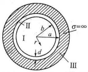 Figure 3: Metallic Wall Circular Waveguide Lined with Dielectric Layer
In 1943, H. Buchholz[18] published the paper "Circular waveguides filled with dielectric matter", which first put forward the problem of the influence of dielectric filled waveguides. In 1950, H. Wachowski and R. Beam[19] published an article entitled "Dielectric rod waveguide with Shielding". In the above paper, the characteristic equation (assuming the conductivity of the waveguide material $\sigma = \infty$ ) when the inner wall of the circular waveguide is artificially added with a uniform dielectric layer (FIG. 3) is derived, which is called the BwB equation. In 1957, Unger[20] proposed a perturbed approximate solution to the BwB equation. These works are called "artificial dielectric layer circular waveguide theory". In 1949, J. Brown[21] published a paper entitled
"Correction of attenuation constant of piston type attenuator", which analyzed the normal mode of circular waveguides with uniform oxide layer on the inner wall, and also assumed that the conductivity of the waveguide material $\sigma = \infty$; The eigen equation derived under this assumption is called Brown equation, and its shape is different from that of BwB equation. In 1993, Zhi-xun Huang and Cheng Zeng[17] published the most general formula, called the Huang Zeng equation.
In early applications, the lined waveguide is mainly used as a long-distance transmission tool in the micro wave and infrared bands, that is, the application of the lined uniform dielectric layer to obtain a small attenuation of the main low-order mode. Later, in the study of mode suppression and how to reduce the radar reflection cross section (RCS), the opposite application of low-loss long-distance transmission has appeared, that is, the use of lining the medium layer to obtain a large attenuation of the main low-order mode; The theoretical basis is that since the internal radiation of the low-order mode in the terminal short-circuit waveguide is the main contribution to RCS, the RCS can be greatly reduced as long as the lined dielectric layer can effectively inhibit the main low-order mode.
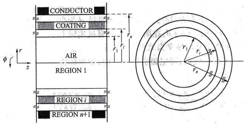 Figure 4: Multi-Layer Dielectric Lined Metal Wall Circular Waveguide
When assuming the physical model, Zhi-xun Huang and Cheng Zeng[14] stipulate that the dielectric lining of the metal-walled circular waveguide can be multi-layered, that is, multilayered coated circular waveguide, as shown in FIG. 4.A difficult mathematical analysis results in the following characteristic equation:
$$
k _ {0} ^ {2} \left(\frac {\varepsilon_ {\mathrm {r} 1}}{h _ {1}} \frac {\mathrm {J} _ {m} ^ {\prime} (u)}{\mathrm {J} _ {m} (u)} - \frac {\varepsilon_ {\mathrm {r} 2}}{h _ {2}} \frac {F _ {e} ^ {\prime} (q)}{F _ {e} (q)}\right) \left(\frac {\mu_ {\mathrm {r} 1}}{h _ {1}} \frac {\mathrm {J} _ {m} ^ {\prime} (u)}{\mathrm {J} _ {m} (u)} - \frac {\mu_ {\mathrm {r} 2}}{h _ {2}} \frac {F _ {h} ^ {\prime} (q)}{F _ {h} (q)}\right) \tag {71}
$$
$$
= \eta_ {b} ^ {2} + \left(R _ {e} (q) R _ {h} (q) \eta_ {a} ^ {2} - \frac {1}{k _ {0} ^ {2}} P _ {2} ^ {2} (q) \eta_ {a} ^ {2} \eta_ {b} ^ {2} + \frac {8 \mu_ {\mathrm {r} 2} \varepsilon_ {\mathrm {r} 2} \eta_ {a} \eta_ {b}}{\pi^ {2} a b h _ {2} ^ {4}}\right) \frac {1}{R _ {e} (q) R _ {h} (q)}
$$
$$
\eta_ {b} = \eta_ {1}, \quad \eta_ {a} = \eta_ {2}
$$
$$
u = h _ {1} b, q = h _ {2} b, v = h _ {3} a
$$
$$
F _ {e} (q) = \frac {\varepsilon_ {\mathrm {r} 2}}{h _ {2}} Q _ {2} (q) - \frac {\varepsilon_ {\mathrm {r} 3}}{h _ {3}} \frac {\mathrm {H} _ {m} ^ {\prime (2)} (\nu)}{\mathrm {H} _ {m} ^ {(2)} (\nu)} P _ {2} (q) \tag {72}
$$
$$
R _ {e} (q) = \frac {\varepsilon_ {\mathrm {r} 2}}{h _ {2}} P _ {2} ^ {\prime} (q) - \frac {\varepsilon_ {\mathrm {r} 3}}{h _ {3}} \frac {\mathbf {H} _ {m} ^ {\prime (2)} (v)}{\mathbf {H} _ {m} ^ {(2)} (v)} P _ {2} (q) \tag {73}
$$
among
$$
P _ {i} \left(h _ {i} r _ {i - 1}\right) = J _ {m} \left(h _ {i} r _ {i - 1}\right) N _ {m} \left(h _ {i} r _ {i}\right) - J _ {m} \left(h _ {i} r _ {i}\right) N _ {m} \left(h _ {i} r _ {i - 1}\right) \tag {74}
$$
$$
Q _ {i} \left(h _ {i} r _ {i - 1}\right) = J _ {m} \left(h _ {i} r _ {i - 1}\right) N _ {m} ^ {\prime} \left(h _ {i} r _ {i}\right) - J _ {m} ^ {\prime} \left(h _ {i} r _ {i}\right) N _ {m} \left(h _ {i} r _ {i - 1}\right) \tag {75}
$$
$$
P _ {i} ^ {\prime} \left(h _ {i} r _ {i - 1}\right) = J _ {m} ^ {\prime} \left(h _ {i} r _ {i - 1}\right) N _ {m} \left(h _ {i} r _ {i}\right) - J _ {m} \left(h _ {i} r _ {i}\right) N _ {m} ^ {\prime} \left(h _ {i} r _ {i - 1}\right) \tag {76}
$$
$$
Q _ {i} ^ {\prime} \left(h _ {i} r _ {i - 1}\right) = J _ {m} ^ {\prime} \left(h _ {i} r _ {i - 1}\right) N _ {m} ^ {\prime} \left(h _ {i} r _ {i}\right) - J _ {m} ^ {\prime} \left(h _ {i} r _ {i}\right) N _ {m} ^ {\prime} \left(h _ {i} r _ {i - 1}\right) \tag {77}
$$
Our new equation can be used to deal with the situation of artificially adding dielectric layer to the inner wall of the circular waveguide, and to analyze the effect of forming oxide layer in the precision cutoff attenuator.
## VII. CALCULATION OF THE INFLUENCE OF OXIDE LAYER ON THE INNER SURFACE OF CIRCULAR WAVEGUIDE[6]
Microwave attenuation measurement technology mainly uses IF instead of the method, that is, the standard cut-off waveguide attenuator as the core, to form a comparable standard at IF (30MHz). If its accuracy reaches $5 \times 10^{-5}$, the overall microwave attenuation measurement accuracy can reach $10^{-3} \sim 10^{-4}$. In short, the circular cut-off waveguide is the heart of the cut-off attenuation standard, and its processing conditions meet the requirements of high precision and low roughness to ensure that the electrical index is qualified. The entire attenuation standard should be placed in a laboratory with constant temperature and humidity. Taking the standard of the National Institute of Metrology (NIM) as an example, the accuracy is $\mathrm{d}A$
$$
= \pm (5 \times 1 0 ^ {- 5} + 0. 0 0 0 2) \mathrm {d B}; \text {T h i s m e a n s t h a t i . e .} \frac {\mathrm {d} \gamma_ {1 1}}{\gamma_ {1 1}}
$$
$= \pm 5\times 10^{-5}$ $\alpha \cdot \mathrm{d}l = 0.0002\mathrm{dB}$. Other indicators are: measuring range $0\sim 120\mathrm{dB}$, resolution $\pm 0.0001\mathrm{dB}$ (0.1mdB). Accordingly, two examples of accuracy data can be calculated: $\pm 0.0007\mathrm{dB} / 10\mathrm{dB}$ (i.e., $\pm 7\times 10^{-5}$ ); $\pm 0.0052\mathrm{dB} / 100\mathrm{dB}$ (i.e. $\pm 5.2\times 10^{-5}$ ). The high resolution length measurement guarantees a reduction of $\mathrm{d}l$ which is due to the use of laser length measurement technology.
Below the national standards, there are so-called secondary standards, which are distributed in various industrial sectors and assume the task of regional standards. The fixed-point same frequency comparison method (based on the medium frequency substitution method) is adopted, which is based on the cut-off attenuator as the core standard component. For example, the domestic T0-7 attenuation standard measuring instrument, its total index is: frequency 1GHz~12.5GHz(fixed intermediate frequency 30MHz after conversion), attenuation range 100dB, attenuation measurement accuracy $5 \times 10^{-4\left[20\right]}$. Specifically for the standard cutoff attenuator, the circular cutoff waveguide is made of H59 brass, the diameter is $2a = 31.962mm$, the diameter machining accuracy is $\pm 5\mu m$, and the internal surface roughness Ra is $0.2\mu m$. Corresponding attenuation constant $\alpha = 1\mathrm{dB / mm}$; The length measurement technique used is raster, not laser, but also achieves high resolution - reading resolution of 0.002dB(2mdB).
For the cut-off waveguide attenuators with accuracy up to $5 \times 10^{-5}$, the oxidation layer on the inner wall of the guided wall is a problem that needs to be considered. The thickness of this oxide layer is small, but it is a factor in error. As mentioned earlier, the relevant equations are the starting point for our analysis. For example, Brown's equation assumes that the oxide film is a pure medium and its dielectric constant is $\varepsilon_0 \sim \infty$. Brown's[21] approximate analysis shows that the error of the propagation constant for $\mathsf{H}_{11}$ mode in the cutoff region is
$$
\frac {\mathrm {d} \gamma_ {1 1}}{\gamma_ {1 1}} = (1 \sim 1. 8) \frac {d}{a} \tag {78}
$$
Where $a$ is the inner diameter of circular waveguide; $\mathbf{d}$ is the oxide film thickness. Therefore, Brown believes that if the attenuation constant error is required to be $< 1\times 10^{-5}$, the oxide film thickness is required to be $\mathbf{d} < 10^{-4}\mathrm{mm}(0.1\mu \mathrm{m})$. These can be called "circular cut-off waveguide theories for naturally occurring thick layers of oxide film".
The characteristics of this section are as follows: 1 The characteristic equation of the metal-walled circular waveguide with dielectric layer is discussed; 2 Brown equation was derived from Buchholz-Wachowski-Beam equation (BWB equation); 3 The perturbation solution $(\mathbf{H}_{\mathrm{mn}}$ mode) of Brown equation is discussed. 4 The case of H-mode below the truncated frequency is further obtained; 5 The reasons for the inconsistency between the two sets of theoretical results are analyzed. 6 The $\mathsf{H}_{11}$ -mode cut-off waveguide is numerically calculated, the influence of oxide layer is numerically analyzed, and the limit of tolerable oxide layer thickness is obtained.
If we follow Figure 3 for discussion, we have $a = b + d$, $\rho = b / a < 1$, $x_1 = h_1a$, $x_2 = h_2a$, $\rho x_1 = h_1b$, $\rho x_2 = h_2b$. Here, is the radial propagation constant:
$$
h _ {1} ^ {2} = + k _ {0} ^ {2} \gamma^ {2}
$$
$$
h _ {2} ^ {2} = k _ {2} ^ {2} + \gamma^ {2} \approx \varepsilon_ {\mathrm {r}} k _ {0} ^ {2} + \gamma^ {2} \tag {79}
$$
Where $\gamma$ is the axial propagation constant: $k_{2}$ is a parameter that characterizes the performance of the medium is:
$$
k _ {2} = \sqrt {\omega^ {2} \varepsilon_ {2} \mu_ {2} - j \omega \mu_ {2} \sigma_ {2}}
$$
Where $\varepsilon_{2}$ is the dielectric constant of the dielectric layer $\mu_{2}$ is the permeability of the dielectric layer, $\mu_{2} = \mu_{\mathrm{r}}\mu_{0}\sigma_{2}$ is the conductivity of the dielectric layer. For the actual medium, $\sigma_{2}\approx 0$ so there are
$$
k _ {2} = \omega \sqrt {\varepsilon_ {2} \mu_ {2}} = k _ {0} \sqrt {\varepsilon_ {\mathrm {r}} \mu_ {\mathrm {r}}}
$$
take the medium $\mu_{\mathrm{r}} = 1$, so get
$$
k _ {2} \approx \sqrt {\varepsilon_ {\mathrm {r}} k _ {0}} \tag {80}
$$
Unger gives the form of the BwB equation as: [12]
$$
m ^ {2} \left[ \frac {1}{x _ {1} ^ {2}} - \frac {1}{x _ {2} ^ {2}} \right] ^ {2} - \rho^ {2} \frac {x _ {2} ^ {2} - x _ {1} ^ {2}}{x _ {2} ^ {2} - \varepsilon_ {\mathrm {r}} x _ {1} ^ {2}} \left[ \frac {1}{x _ {1}} \frac {\mathbf {J} _ {m} ^ {\prime} (\rho x _ {1})}{\mathbf {J} _ {m} (\rho x _ {1})} + \frac {\varepsilon_ {\mathrm {r}} \mathbf {W} _ {m} (\rho x _ {2})}{\rho x _ {2} ^ {2} \mathbf {U} _ {m} (\rho x _ {2})} \right] \cdot \left[ \frac {1}{x _ {1}} \frac {\mathbf {J} _ {m} ^ {\prime} (\rho x _ {1})}{\mathbf {J} _ {m} (\rho x _ {1})} + \frac {1}{\rho x _ {2} ^ {2}} \frac {\mathbf {V} _ {m} (\rho x _ {2})}{\mathbf {Z} _ {m} (\rho x _ {2})} \right] = 0 \tag {81}
$$
$$
\mathrm {U} _ {m} (\rho x _ {2}) = J _ {m} (\rho x _ {2}) N _ {m} (x _ {2}) - N _ {m} (\rho x _ {2}) J _ {m} (x _ {2})
$$
$$
\mathrm {V} _ {m} (\rho x _ {2}) = \rho x _ {2} ^ {2} \left[ \mathrm {J} _ {m} ^ {\prime} (\rho x _ {2}) N _ {m} ^ {\prime} (x _ {2}) - N _ {m} ^ {\prime} (\rho x _ {2}) \mathrm {J} _ {m} ^ {\prime} (x _ {2}) \right]
$$
$$
\mathrm {W} _ {m} (\rho x _ {2}) = \rho x _ {2} ^ {2} [ J _ {m} (x _ {2}) N _ {m} ^ {\prime} (\rho x _ {2}) - \mathrm {J} _ {m} ^ {\prime} (\rho x _ {2}) N _ {m} (x _ {2}) ]
$$
$$
Z _ {m} \left(\rho x _ {2}\right) = x _ {2} \left[ J _ {m} ^ {\prime} \left(x _ {2}\right) N _ {m} \left(\rho x _ {2}\right) - J _ {m} \left(\rho x _ {2}\right) N _ {m} ^ {\prime} \left(x _ {2}\right) \right]
$$
Now we want to transform the formula, for example
$$
\rho^ {2} \frac {x _ {2} ^ {2} - x _ {1} ^ {2}}{x _ {2} ^ {2} - \varepsilon_ {\mathrm {r}} x _ {1} ^ {2}} = \rho^ {2} \frac {h _ {2} ^ {2} - h _ {1} ^ {2}}{h _ {2} ^ {2} - \varepsilon_ {\mathrm {r}} h _ {1} ^ {2}} = \rho^ {2} \frac {\left(\varepsilon_ {\mathrm {r}} - 1\right) k _ {0} ^ {2}}{\left(1 - \varepsilon_ {\mathrm {r}}\right) \gamma^ {2}} = \rho^ {2} \frac {k _ {0} ^ {2}}{- \gamma^ {2}} = \frac {k _ {0} ^ {2} b ^ {2}}{k _ {\mathrm {z}} ^ {2} a ^ {2}}
$$
again, let's deal with the following items:
$$
\frac {\varepsilon_ {\mathrm {r}}}{\rho x _ {2} ^ {2}} \frac {\mathrm {W} _ {m} (\rho x _ {2})}{\mathrm {U} _ {m} (\rho x _ {2})} = \frac {\varepsilon_ {\mathrm {r}}}{x _ {2}} \frac {\mathrm {J} _ {m} (x _ {2}) N _ {m} ^ {\prime} (\rho x _ {2}) - \mathrm {J} _ {m} ^ {\prime} (\rho x _ {2}) N _ {m} (x _ {2})}{\mathrm {J} _ {m} (\rho x _ {2}) N _ {m} (x _ {2}) - N _ {m} (\rho x _ {2}) J _ {m} (x _ {2})} - \frac {\varepsilon_ {\mathrm {r}}}{h _ {2} a} \frac {\mathrm {J} _ {m} ^ {\prime} (h _ {2} b) N _ {m} (h _ {2} a) - J _ {m} (h _ {2} a) N _ {m} ^ {\prime} (h _ {2} b)}{\mathrm {J} _ {m} (h _ {2} b) N _ {m} (h _ {2} a) - J _ {m} (h _ {2} a) N _ {m} (h _ {2} b)}
$$
It is
$$
P _ {m} \left(h _ {2} r\right) = J _ {m} \left(h _ {2} r\right) N _ {m} \left(h _ {2} a\right) - J _ {m} \left(h _ {2} a\right) N _ {m} \left(h _ {2} r\right)
$$
where $r$ represents radial coordinates. Then there is
$$
P _ {m} \left(h _ {2} b\right) = J _ {m} \left(h _ {2} b\right) N _ {m} \left(h _ {2} a\right) - J _ {m} \left(h _ {2} a\right) N _ {m} \left(h _ {2} b\right)
$$
$$
P _ {m} ^ {\prime} \left(h _ {2} b\right) = J _ {m} ^ {\prime} \left(h _ {2} b\right) N _ {m} \left(h _ {2} a\right) - J _ {m} \left(h _ {2} a\right) N _ {m} ^ {\prime} \left(h _ {2} b\right)
$$
Therefore available
$$
\frac {\varepsilon_ {r}}{\rho x _ {2} ^ {2}} \frac {\mathrm {W} _ {m} (\rho x _ {2})}{\mathrm {U} _ {m} (\rho x _ {2})} = - \frac {\varepsilon_ {r}}{h _ {2} a} \frac {P _ {m} ^ {\prime} (h _ {2} b)}{P _ {m} (h _ {2} b)}
$$
It is
$$
Q _ {m} \left(h _ {2} r\right) = J _ {m} \left(h _ {2} r\right) N _ {m} ^ {\prime} \left(h _ {2} a\right) - J _ {m} ^ {\prime} \left(h _ {2} a\right) N _ {m} \left(h _ {2} r\right)
$$
the same can be proved:
$$
\frac {1}{\rho x _ {2} ^ {2}} \frac {\mathrm {V} _ {m} (\rho x _ {2})}{\mathrm {Z} _ {m} (\rho x _ {2})} = - \frac {1}{h _ {2} a} \frac {Q _ {m} ^ {\prime} (h _ {2} b)}{Q _ {m} (h _ {2} b)}
$$
After this kind of sorting, the BwB equation becomes
$$
\left[ \frac {1}{h _ {1}} \frac {\mathrm {J} _ {m} ^ {\prime} \left(h _ {1} b\right)}{\mathrm {J} _ {m} \left(h _ {1} b\right)} - \frac {\varepsilon_ {\mathrm {r}}}{h _ {2}} \frac {P _ {m} ^ {\prime} \left(h _ {2} b\right)}{P _ {m} \left(h _ {2} b\right)} \right] \cdot \left[ \frac {1}{h _ {1}} \frac {\mathrm {J} _ {m} ^ {\prime} \left(h _ {1} b\right)}{\mathrm {J} _ {m} \left(h _ {1} b\right)} - \frac {\mu_ {\mathrm {r}}}{h _ {2}} \frac {Q _ {m} ^ {\prime} \left(h _ {2} b\right)}{Q _ {m} \left(h _ {2} b\right)} \right] = \frac {m ^ {2}}{b ^ {2}} \frac {k _ {\mathrm {z}} ^ {2}}{k _ {0} ^ {2}} \left[ \frac {1}{h _ {1} ^ {2}} - \frac {1}{h _ {2} ^ {2}} \right] ^ {2} \tag {82}
$$
the above formula is strict when the waveguide material is ideally conductive $(\sigma = \infty)$.
We tried to derive the Brown equation from the BwB equation, and now we have
$$
h _ {1} a = h _ {1} b + h _ {1} d
$$
$$
h _ {2} a = h _ {2} b + h _ {2} d
$$
Suppose $d \ll b$, cylindrical functions can be expanded by variables. $\mathbf{h}_1b$ and $\mathbf{h}_2b$. The Taylor series shows:
$$
f \left(x _ {0} + \Delta\right) = f \left(x _ {0}\right) + f ^ {\prime} \left(x _ {0}\right) \Delta + \frac {1}{2 !} f ^ {\prime} \left(x _ {0}\right) \Delta^ {2} + \dots
$$
linear expansion is preferable if $\Delta$ small:
$$
f \left(x _ {0} + \Delta\right) = f \left(x _ {0}\right) + f ^ {\prime} \left(x _ {0}\right) \Delta
$$
Therefore there may be
$$
J _ {m} \left(h _ {2} a\right) = J _ {m} \left(h _ {2} b\right) + h _ {2} d J _ {m} ^ {\prime} \left(h _ {2} b\right)
$$
$$
\mathbf {J} _ {m} ^ {\prime} \left(h _ {2} a\right) = \mathbf {J} _ {m} ^ {\prime} \left(h _ {2} b\right) + h _ {2} d \mathbf {J} _ {m} ^ {\prime \prime} \left(h _ {2} b\right)
$$
The second type of Bessel function also has a similar relationship, so it can be proved that:
$$
\frac {P _ {m} ^ {\prime} \left(h _ {2} b\right)}{P _ {m} \left(h _ {2} b\right)} \approx - \frac {1}{h _ {2} d} \tag {83}
$$
Now we need to utilize the Wronsky relation of the integer order Bessel function:
$$
\mathrm {J} _ {m} (x) N _ {m} ^ {\prime} (x) - \mathrm {J} _ {m} ^ {\prime} (x) N _ {m} (x) = \mathrm {J} _ {m + 1} (x) N _ {m} (x) - \mathrm {J} _ {m} (x) N _ {m + 1} (x) = \mathrm {J} _ {m} (x) N _ {m - 1} (x) - \mathrm {J} _ {m - 1} (x) N _ {m} (x) = \frac {2}{\pi x}
$$
and
$$
\mathrm {J} _ {m} (x) N _ {m} ^ {\prime \prime} (x) - \mathrm {J} _ {m} ^ {\prime \prime} (x) N _ {m} (x) = - \frac {2}{\pi x ^ {2}}
$$
$$
\mathrm {J} _ {m} ^ {\prime} (x) N _ {m} ^ {\prime \prime} (x) - \mathrm {J} _ {m} ^ {\prime \prime} (x) N _ {m} ^ {\prime} (x) = \frac {2}{\pi x} \left(1 - \frac {m ^ {2}}{x ^ {2}}\right)
$$
It can therefore be proved that:
$$
\frac {Q _ {m} ^ {\prime} \left(h _ {2} b\right)}{Q _ {m} \left(h _ {2} b\right)} \approx h _ {2} d \left(1 - \frac {m ^ {2}}{h _ {2} ^ {2} b ^ {2}}\right) \tag {84}
$$
The following symbols are also introduced:
$$
u = h _ {1} b = b \sqrt {k _ {0} ^ {2} + \gamma^ {2}} \tag {85}
$$
$$
q = h _ {2} b = b \cdot \overline {{k _ {2} ^ {2} + \gamma^ {2}}} \tag {86}
$$
and consider the following relationship:
$$
k _ {z} ^ {2} = - \gamma^ {2}
$$
This style (82) can be arranged as
$$
- \left[ k _ {0} ^ {2} \frac {\mathrm {J} _ {m} ^ {\prime} (u)}{\mathrm {J} _ {m} (u)} + \frac {b u k _ {2} ^ {2}}{\mu_ {1} d q ^ {2}} \right] \cdot \left[ \frac {\mathrm {J} _ {m} ^ {\prime} (u)}{\mathrm {J} _ {m} (u)} - \frac {\mu_ {r} u d}{b} \left(1 - \frac {m ^ {2}}{q ^ {2}}\right) \right] = m ^ {2} \gamma^ {2} u ^ {2} \left(\frac {1}{u ^ {2}} - \frac {1}{q ^ {2}}\right) ^ {2}
$$
can also be written as
$$
- \left[ \frac {k _ {0} ^ {2}}{\mu_ {0}} \frac {\mathrm {J} _ {m} ^ {\prime} (u)}{\mathrm {J} _ {m} (u)} + \frac {b u k _ {2} ^ {2}}{d q ^ {2} \mu_ {2}} \right] \cdot \left[ \mu_ {0} \frac {\mathrm {J} _ {m} ^ {\prime} (u)}{\mathrm {J} _ {m} (u)} - \frac {\mu_ {r} u d}{b} \left(1 - \frac {m ^ {2}}{q ^ {2}}\right) \right] = \frac {m ^ {2} \gamma^ {2}}{u ^ {2}} \left[ 1 - \frac {u ^ {2}}{q ^ {2}} \right] ^ {2} \tag {87}
$$
this is Brown's characteristic equation. The error only comes from ignoring small quantities of higher order during linear expansion, which requires very little (the oxide film is very thin). Brown's equation is correct, but it cannot be used for film thickness.
Equation (87) can also be written as
$$
\left[ \frac {k _ {0} ^ {2}}{\mu_ {0}} \frac {\mathrm {J} _ {m} ^ {\prime} (u)}{\mathrm {J} _ {m} (u)} + \frac {b u k _ {2} ^ {2}}{d q ^ {2} \mu_ {2}} \right] \cdot \left[ \mu_ {0} \frac {\mathrm {J} _ {m} ^ {\prime} (u)}{\mathrm {J} _ {m} (u)} - \frac {\mu_ {r} u d}{b} \left(1 - \frac {m ^ {2}}{q ^ {2}}\right) \right] = \frac {m ^ {2} k _ {\mathrm {z}} ^ {2}}{u ^ {2}} \left[ 1 - \frac {u ^ {2}}{q ^ {2}} \right] ^ {2} \tag {88}
$$
Now the perturbation solution of Brown's equation is required; Multiply the left side of the formula and expand it, multiply the left and right side by $d / b$, omit the $(d / b)^2$ term, and set $\delta = d / b$ to obtain the approximate equation:
$$
k _ {2} ^ {2} \frac {\mu_ {0}}{\mu_ {2}} \left[ \frac {\mathbf {J} _ {m} ^ {\prime} (u)}{\mathbf {J} _ {m} (u)} \right] + k _ {0} ^ {2} \delta \left[ \frac {\mathbf {J} _ {m} ^ {\prime} (u)}{\mathbf {J} _ {m} (u)} \right] ^ {2} - k _ {2} ^ {2} \frac {u ^ {2}}{q ^ {2}} \delta \left(1 - \frac {m ^ {2}}{q ^ {2}}\right) - m ^ {2} k _ {z} ^ {2} u ^ {2} \delta \left(\frac {1}{u ^ {2}} - \frac {1}{q ^ {2}}\right) ^ {2} = 0 \tag {89}
$$
It is actually
$$
f (u) = 0 (9 0)
$$
now we're going to approximate it. For the sake of comparison with Brown's original text, using one of his symbols, it is actually:
$$
h _ {m n} = j \gamma_ {m n} \tag {91}
$$
hence
$$
h _ {m n} ^ {2} = k _ {0} ^ {2} - \frac {u _ {m n} ^ {2}}{b ^ {2}} \tag {92}
$$
perturbation is for $\delta = 0$ (no oxide film present). Case of $\delta = 0$:
$$
\mathrm {J} _ {m} ^ {\prime} (u) = 0
$$
let the root be
$$
u _ {m n} = k _ {m n}
$$
when a thin oxide film is present, perturbations are generated:
$$
u _ {m n} = + k _ {m n} \mathrm {d} u _ {m n} \tag {93}
$$
now we're going to do the Newton-Raphson process, which is
$$
\mathrm {d} u _ {m n} \approx - \frac {f \left(k _ {m n}\right)}{f ^ {\prime} \left(k _ {m n}\right)} \tag {94}
$$
However, it can be proved that:
$$
\frac {\mathrm {d} h _ {m n}}{h _ {m n}} = - \frac {u _ {m n}}{b ^ {2} h _ {m n} ^ {2}} \mathrm {d} u _ {m n} \tag {95}
$$
and
$$
\frac {\mathrm {d} h _ {m n}}{h _ {m n}} = \frac {\mathrm {d} \gamma_ {m n}}{\gamma_ {m n}} \tag {96}
$$
So when $u_{mn} = k_{mn}$,
$$
\frac {\mathrm {d} \gamma_ {m n}}{\gamma_ {m n}} = - \frac {k _ {m n} ^ {2}}{b ^ {2} h _ {m n} ^ {2}} \mathrm {d} u _ {m n} = \frac {k _ {m n}}{b ^ {2} h _ {m n} ^ {2}} \frac {f \left(k _ {m n}\right)}{f ^ {\prime} \left(k _ {m n}\right)} \tag {97}
$$
So let's figure $\mathbf{d}\pmb{u}_{mn}$ out first. From formula (89), when $\mathbf{J}_m^{\prime}(\mathbf{u}) = 0$
$$
f (u) = - k _ {2} ^ {2} \frac {u ^ {2}}{q ^ {2}} \left(1 - \frac {m ^ {2}}{q ^ {2}}\right) \delta - m ^ {2} k _ {\mathrm {z}} ^ {2} u ^ {2} \left[ \frac {1}{u ^ {2}} - \frac {1}{q ^ {2}} \right] ^ {2} \delta
$$
Thus obtained
$$
f \left(k _ {m n}\right) = - k _ {2} ^ {2} \frac {k _ {m n} ^ {2}}{q _ {m n} ^ {2}} \left(1 - \frac {m ^ {2}}{q _ {m n} ^ {2}}\right) \delta - \left(k _ {2} ^ {2} \frac {\delta}{q _ {m n} ^ {2}}\right) \frac {m ^ {2} k _ {z} ^ {2} k _ {m n} ^ {2} q _ {m n} ^ {2}}{k _ {2} ^ {2}} \left[ \frac {1}{k _ {m n} ^ {2}} - \frac {1}{q _ {m n} ^ {2}} \right] ^ {2}
$$
replace it with $k_{z}^{2}$, and arrange it $h_{mn}^{2}$
$$
f \left(k _ {m n}\right) = - k _ {2} ^ {2} \frac {\delta}{q _ {m n} ^ {2}} \left\{k _ {m n} ^ {2} \left(1 - \frac {m ^ {2}}{q _ {m n} ^ {2}}\right) + \frac {m ^ {2} h _ {m n} ^ {2} q _ {m n} ^ {2}}{k _ {2} ^ {2} k _ {m n} ^ {2}} \left(1 - \frac {k _ {m n} ^ {2}}{q _ {m n} ^ {2}}\right) ^ {2} \right\} \tag {98}
$$
look below; $f^{\prime}(k_{mn})$ Just take the first term of formula (89) (zero-order approximation) and set then there is $\mu_2 = \mu_0$,
$$
f (u) = k _ {2} ^ {2} \frac {u}{q ^ {2}} \left[ \frac {\mathrm {J} _ {m} ^ {\prime} (u)}{\mathrm {J} _ {m} (u)} \right]
$$
The expression is obtained by solving according to the differential rule obtain $\mathbf{f}'(u)$, and then $J_{\mathrm{m}}'(\mathbf{k}_{\mathrm{mn}})$ equal to 0, so that's it
$$
f ^ {\prime} \left(k _ {m n}\right) = \frac {k _ {2} ^ {2}}{q _ {m n} ^ {2}} k _ {m n} \frac {\mathrm {J} _ {m} ^ {\prime \prime} \left(k _ {m n}\right)}{\mathrm {J} _ {m} \left(k _ {m n}\right)}
$$
Using the Bessel recurrence formula:
$$
\mathrm {J} _ {m} ^ {\prime \prime} \left(k _ {m n}\right) = - \left(1 - \frac {m ^ {2}}{k _ {m n} ^ {2}}\right) \mathrm {J} _ {m} \left(k _ {m n}\right)
$$
$$
f ^ {\prime} \left(k _ {m n}\right) = - \frac {k _ {2} ^ {2}}{q _ {m n} ^ {2}} k _ {m n} \left(1 - \frac {m ^ {2}}{k _ {m n} ^ {2}}\right) \tag {99}
$$
thus obtained
$$
\frac {\mathrm {d} \gamma_ {m n} ^ {(b)}}{\gamma_ {m n} ^ {(b)}} \approx \frac {\delta}{h _ {m n} ^ {2} b ^ {2}} \left[ k _ {m n} ^ {2} \left(1 - \frac {m ^ {2}}{q _ {m n} ^ {2}}\right) + \frac {m ^ {2} h _ {m n} ^ {2} q _ {m n} ^ {2}}{k _ {2} ^ {2} k _ {m n} ^ {2}} \left(1 - \frac {k _ {m n} ^ {2}}{q _ {m n} ^ {2}}\right) ^ {2} \right] \frac {k _ {m n} ^ {2}}{k _ {2} ^ {2} - m ^ {2}} \tag {100}
$$
$h_{mn}$: obtained from formula (92)
$$
h _ {m n} ^ {2} = k _ {0} ^ {2} - \frac {k _ {m n} ^ {2}}{b ^ {2}} \tag {101}
$$
It can be determined by the following formula: $q_{mn}$
$$
q _ {m n} ^ {2} = k _ {2} ^ {2} b ^ {2} + \gamma_ {m n} ^ {2} b ^ {2} = k _ {2} ^ {2} b ^ {2} - h _ {m n} ^ {2} b ^ {2} = k _ {2} ^ {2} b ^ {2} - k _ {0} ^ {2} b ^ {2} + k _ {m n} ^ {2} \tag {102}
$$
These results are consistent with Brown's.
The opposite formula (100) can be deformed. On account of
$$
k _ {m n} ^ {2} - \frac {m ^ {2} k _ {m n} ^ {2}}{q _ {m n} ^ {2}} = \left(k _ {m n} ^ {2} - m ^ {2}\right) + m ^ {2} \left(1 - \frac {k _ {m n} ^ {2}}{q _ {m n} ^ {2}}\right) = \left(k _ {m n} ^ {2} - m ^ {2}\right) + m ^ {2} k _ {m n} ^ {2} \left(\frac {1}{k _ {m n} ^ {2}} - \frac {1}{q _ {m n} ^ {2}}\right)
$$
So the equation (100) can be written as
$$
\frac {\mathrm {d} \gamma_ {m n} ^ {(b)}}{\gamma_ {m n} ^ {(b)}} = \frac {\delta k _ {m n} ^ {2}}{h _ {m n} ^ {2} b ^ {2}} + \frac {m ^ {2} \delta}{h _ {m n} ^ {2} b ^ {2}} \left\{k _ {m n} ^ {2} \left(\frac {1}{k _ {m n} ^ {2}} - \frac {1}{q _ {m n} ^ {2}}\right) + \frac {k _ {m n} ^ {2} q _ {m n} ^ {2}}{k _ {2} ^ {2} k _ {m n} ^ {2}} \left(1 - \frac {k _ {m n} ^ {2}}{q _ {m n} ^ {2}}\right) ^ {2} \right\} \frac {k _ {m n} ^ {2}}{k _ {m n} ^ {2} - m ^ {2}}
$$
where The symbol $(\pmb{b})$ indicates that this result is obtained by expanding the reference radius (not). The second term on the right can be simplified to
$$
\frac {m ^ {2} \delta}{h _ {m n} ^ {2} b ^ {2}} \left\{\frac {q _ {m n} ^ {2} - k _ {m n} ^ {2}}{q _ {m n} ^ {2}} + \frac {h _ {m n} ^ {2} \left(q _ {m n} ^ {2} - k _ {m n} ^ {2}\right)}{k _ {2} ^ {2} k _ {m n} ^ {2} q _ {m n} ^ {2}} \right\} \frac {k _ {m n} ^ {2}}{k _ {m n} ^ {2} - m ^ {2}} = \frac {m ^ {2} \delta}{h _ {m n} ^ {2} b ^ {2}} \frac {q _ {m n} ^ {2} - k _ {m n} ^ {2}}{k _ {m n} ^ {2} - m ^ {2}} \left\{\frac {k _ {2} ^ {2} k _ {m n} ^ {2} + h _ {m n} ^ {2} \left(q _ {m n} ^ {2} - k _ {m n} ^ {2}\right)}{k _ {2} ^ {2} q _ {m n} ^ {2}} \right\}
$$
however
$$
q _ {m n} ^ {2} - k _ {m n} ^ {2} = k _ {0} ^ {2} b ^ {2} \left(\varepsilon_ {\mathrm {r}} - 1\right) \tag {103}
$$
It can therefore be proved that:
$$
k _ {2} ^ {2} k _ {m n} ^ {2} + h _ {m n} ^ {2} \left(q _ {m n} ^ {2} - k _ {m n} ^ {2}\right) = k _ {0} ^ {2} q _ {m n} ^ {2} \tag {104}
$$
we plug in these results
$$
\frac {\mathrm {d} \gamma_ {m n} ^ {(b)}}{\gamma_ {m n} ^ {(b)}} = \frac {\delta k _ {m n} ^ {2}}{h _ {m n} ^ {2} b ^ {2}} + \frac {m ^ {2} \delta}{h _ {m n} ^ {2} b ^ {2}} - \frac {q _ {m n} ^ {2} - k _ {m n} ^ {2}}{k _ {m n} ^ {2} - m ^ {2}} = \frac {k _ {0} ^ {2}}{k _ {2} ^ {2}} \frac {\delta k _ {m n} ^ {2}}{h _ {m n} ^ {2} b ^ {2}} + m ^ {2} \delta \frac {\varepsilon_ {\mathrm {r}} - 1}{k _ {m n} ^ {2} - m ^ {2}} \frac {k _ {0} ^ {2}}{k _ {2} ^ {2}} \frac {k _ {0} ^ {2}}{h _ {m n} ^ {2}}
$$
However $k_{0}^{2}, k_{2}^{2} - \varepsilon_{r}$, In addition can be ordered
$$
G _ {m n} ^ {2} = \frac {h _ {m n} ^ {2}}{k _ {0} ^ {2}} = 1 - \frac {k _ {m n} ^ {2}}{b ^ {2} k _ {0} ^ {2}} = \frac {1 - \frac {\lambda^ {2}}{\left(\frac {2 \pi b}{k _ {m n}}\right) ^ {2}}}{1 - \frac {\lambda^ {2}}{\lambda_ {c . m n} ^ {2}}}
$$
hence
$$
\frac {\mathrm {d} \gamma_ {m n} ^ {(b)}}{\gamma_ {m n} ^ {(b)}} = \frac {\delta k _ {m n} ^ {2}}{h _ {m n} ^ {2} b ^ {2}} + m ^ {2} \delta \frac {\varepsilon_ {\mathrm {r}} - 1}{\varepsilon_ {\mathrm {r}}} \frac {1}{\left(k _ {m n} ^ {2} - m ^ {2}\right)} G _ {m n} ^ {2}
$$
however
$$
F _ {m n} ^ {2} = \frac {h _ {m n} ^ {2} b ^ {2}}{k _ {m n} ^ {2}} = \frac {b ^ {2} k _ {0} ^ {2}}{k _ {m n} ^ {2}} - 1 = \left(\frac {2 \pi b}{k _ {m n}}\right) ^ {2} \frac {1}{\lambda^ {2}} - 1 = \frac {\lambda_ {c . m n} ^ {2}}{\lambda^ {2}} - 1 \tag {105}
$$
So finally get
$$
\frac {\mathrm {d} \gamma_ {m n} ^ {(b)}}{\gamma_ {m n} ^ {(b)}} = \frac {\delta}{F _ {m n} ^ {2}} + \frac {m ^ {2} \delta \left(\varepsilon_ {\mathrm {r}} - 1\right)}{\varepsilon_ {\mathrm {r}} \left(k _ {m n} ^ {2} - m ^ {2}\right) G _ {m n} ^ {2}} \tag {106}
$$
This expression is relatively comprehensive, Brown has not given such a clear expression.
## VIII. ANALYSIS OF CIRCULAR CUT-OFF WAVEGUIDE AND $\mathsf{H}_{11}^{-}$ MODE
Approximation theory still admits that positive scale can exist. Start with a clear formula, which is obtained from equation
$$
\frac {\mathrm {d} \gamma_ {m n} ^ {(b)}}{\gamma_ {m n} ^ {(b)}} = \frac {d / b}{\left(\frac {\lambda_ {c . m n}}{\lambda}\right) ^ {2} - 1} + \frac {d}{b} \frac {m ^ {2}}{k _ {m n} ^ {2} - m ^ {2}} \left(1 - \frac {1}{\varepsilon_ {\mathrm {r}}}\right) \frac {1}{1 - \left(\frac {\lambda}{\lambda_ {c . m n}}\right) ^ {2}} \tag {107}
$$
Let $m = n = 1$, get the formula applicable to $\mathsf{H}_{11}$ mode
$$
\frac {\mathrm {d} \gamma_ {1 1} ^ {(b)}}{\gamma_ {1 1} ^ {(b)}} = \frac {d / b}{\left(\frac {\lambda_ {c . 1 1}}{\lambda}\right) ^ {2} - 1} + \frac {d}{b} \frac {1}{k _ {1 1} ^ {2} - 1} \left(1 - \frac {1}{\varepsilon_ {\mathrm {r}}}\right) \frac {1}{1 - \left(\frac {\lambda}{\lambda_ {c . 1 1}}\right) ^ {2}} \tag {108}
$$
For the specific case of the cut-off waveguide attenuation standard, $\lambda \gg \lambda_{\mathrm{c}}$, it is obtained
$$
\frac {\mathrm {d} \gamma_ {1 1} ^ {(b)}}{\gamma_ {1 1} ^ {(b)}} \approx - \frac {d}{b} - \frac {d}{b} \frac {1}{k _ {1 1} ^ {2} - 1} \left(1 - \frac {1}{\varepsilon_ {\mathrm {r}}}\right) \left(\frac {\lambda_ {c . 1 1}}{\lambda}\right) ^ {2} \tag {109}
$$
Obviously, the second term on the right side of the equation is small, so
$$
\frac {\mathrm {d} \gamma_ {1 1} ^ {(b)}}{\gamma_ {1 1} ^ {(b)}} \approx - \frac {d}{b} \tag {110}
$$
The minus sign indicates that the oxidation film reduces the attenuation constant.
Now proceed from equation (24) of Brown's paper[13]; Let $\mu_{2} = \mu_{0}$, $m = n = 1$, then the formula becomes
$$
\frac {\mathrm {d} \gamma_ {1 1} ^ {(b)}}{\gamma_ {1 1} ^ {(b)}} = \frac {d}{b} \frac {1}{h _ {1 1} ^ {2} b ^ {2}} \frac {k _ {1 1} ^ {2}}{k _ {1 1} ^ {2} - 1} \left\{k _ {1 1} ^ {2} \left(1 - \frac {1}{q _ {1 1} ^ {2}}\right) + \frac {h _ {1 1} ^ {2} q _ {1 1} ^ {2}}{k _ {2} ^ {2} k _ {1 1} ^ {2}} \left(1 - \frac {k _ {1 1} ^ {2}}{q _ {1 1} ^ {2}}\right) ^ {2} \right\}
$$
Brown, however, "takes the unperturbed decay constant $\mathbf{k}_{11} / b$," which has two caveats.
1. This assumption is only true if the terms $\mathbf{k}_0$ in the formula are ignored. By numerical verification, it is proved that it is allowed to work in the cut-off area.
2. Brown lost a minus sign and should have taken it instead
$$
h _ {1 1} ^ {2} b ^ {2} = - k _ {1 1} ^ {2} \tag {111}
$$
hence
$$
\frac {\mathrm {d} \gamma_ {1 1} ^ {(b)}}{\gamma_ {1 1} ^ {(b)}} = - \frac {d}{b} \frac {k _ {1 1} ^ {2}}{k _ {1 1} ^ {2} - 1} \left\{1 - \frac {1}{q _ {1 1} ^ {2}} + \frac {h _ {1 1} ^ {2} q _ {1 1} ^ {2}}{k _ {2} ^ {2}} \left(\frac {1}{k _ {1 1} ^ {2}} - \frac {1}{q _ {1 1} ^ {2}}\right) ^ {2} \right\} = - \frac {d}{b} \frac {k _ {1 1} ^ {2}}{k _ {1 1} ^ {2} - 1} \left\{1 - \frac {1}{q _ {1 1} ^ {2}} - \frac {q _ {1 1} ^ {2}}{b ^ {2} k _ {2} ^ {2} k _ {1 1} ^ {2}} + \frac {2}{b ^ {2} k _ {2} ^ {2}} - \frac {k _ {1 1} ^ {2}}{b ^ {2} k _ {2} ^ {2} q _ {1 1} ^ {2}} \right\} \tag {112}
$$
If $\varepsilon_{\mathrm{r}} \gg 1$ is assumed, then $\mathbf{k}_2^2 \gg \mathbf{k}_0^2$, therefore desirable:
$$
q _ {1 1} ^ {2} = \approx b ^ {2} k _ {2} ^ {2} - b ^ {2} k _ {0} ^ {2} + k _ {1 1} ^ {2} b ^ {2} k _ {2} ^ {2} + k _ {1 1} ^ {2} \tag {113}
$$
Hence there
$$
\frac {q _ {1 1} ^ {2}}{b ^ {2} k _ {2} ^ {2} k _ {1 1} ^ {2}} + \frac {k _ {1 1} ^ {2}}{b ^ {2} k _ {2} ^ {2} q _ {1 1} ^ {2}} = \frac {b ^ {2} k _ {2} ^ {2} + k _ {1 1} ^ {2}}{b ^ {2} k _ {2} ^ {2} k _ {1 1} ^ {2}} + \frac {q _ {1 1} ^ {2} - b ^ {2} k _ {2} ^ {2}}{b ^ {2} k _ {2} ^ {2} q _ {1 1} ^ {2}} = \frac {1}{k _ {1 1} ^ {2}} + \frac {2}{b ^ {2} k _ {2} ^ {2}} - \frac {1}{q _ {1 1} ^ {2}}
$$
You get it when you plug it in
$$
\frac {\mathrm {d} \gamma_ {1 1} ^ {(b)}}{\gamma_ {1 1} ^ {(b)}} \approx - \frac {d}{b} \tag {114}
$$
This result is correct, and Brown's original formula is:
$$
\frac {\mathrm {d} h _ {1 1}}{h _ {1 1}} = \frac {d}{b} \frac {1}{k _ {1 1} ^ {2} - 1} \left\{\frac {k _ {1 1} ^ {4} - k _ {1 1} ^ {2} + b ^ {2} k _ {2} ^ {2} (k _ {1 1} ^ {2} + 1)}{k _ {1 1} ^ {2} + b ^ {2} k _ {2} ^ {2}} \right\}
$$
this is wrong, because of the loss of a minus sign. Brown is wrong, but his conclusion is still correct on an order of magnitude scale.
We discuss the perturbation of BwB equation
$(\mathsf{H}^{mn}$ -mode) and $\mathsf{H}_{11}$ -mode cases. There is now
$$
k _ {2} ^ {2} \frac {u}{x _ {2} ^ {2}} \left[ \frac {\mathrm {J} _ {m} ^ {\prime} (u)}{\mathrm {J} _ {m} (u)} \right] + k _ {0} ^ {2} \delta \left[ \frac {\mathrm {J} _ {m} ^ {\prime} (u)}{\mathrm {J} _ {m} (u)} \right] ^ {2} - k _ {2} ^ {2} \frac {u ^ {2}}{x _ {2} ^ {2}} \delta \mathrm {K} - m ^ {2} h _ {m n} ^ {2} u ^ {2} \delta \left[ \frac {1}{u ^ {2}} - \frac {1}{x _ {2} ^ {2}} \right] ^ {2} = 0 \tag {117}
$$
$$
h _ {1} b = h _ {1} a - h _ {1} d
$$
$$
h _ {2} b = h _ {2} a - h _ {2} d
$$
Suppose $d \ll a$, cylindrical functions can be expanded by variables $\mathbf{h}_1\mathbf{a}$ 、 $\mathbf{h}_2\mathbf{a}$. Introduce the following symbols:
$$
u = h _ {1} a = a \sqrt {k _ {0} ^ {2} + \gamma^ {2}} \tag {115}
$$
$$
x _ {2} = h _ {2} a = a \sqrt {k _ {2} ^ {2} + \gamma^ {2}} \tag {116}
$$
And let $\delta = d / a$, similar analysis is obtained
The term $\delta^2$ was omitted from the derivation. Where $K$ is
$$
K = \frac {\mathrm {J} _ {m} ^ {\prime} (u)}{\mathrm {J} _ {m} (u)} + \left(1 - \frac {m ^ {2}}{x _ {2} ^ {2}}\right) \tag {118}
$$
Take formula (117) as
$$
f (u) = 0 \tag {119}
$$
It can be proved that:
$$
\frac {\mathrm {d} \gamma_ {m n} ^ {(a)}}{\gamma_ {m n} ^ {(a)}} = - \frac {k _ {m n}}{a ^ {2} h _ {m n} ^ {2}} \mathrm {d} u _ {m n} \tag {120}
$$
It can also be proved that:
$$
\frac {\mathrm {d} \gamma_ {m n} ^ {(a)}}{\gamma_ {m n} ^ {(a)}} = \frac {m ^ {2} \delta}{h _ {m n} ^ {2} a ^ {2}} \left\{1 - \frac {k _ {m n} ^ {2}}{x _ {2 . m n} ^ {2}} + \frac {h _ {m n} ^ {2} x _ {2 . m n} ^ {2}}{k _ {2} ^ {2} k _ {m n} ^ {2}} \left[ 1 - \frac {k _ {m n} ^ {2}}{x _ {2 . m n} ^ {2}} \right] ^ {2} \right\} \frac {k _ {m n} ^ {2}}{k _ {m n} ^ {2} - m ^ {2}} \tag {121}
$$
and
$$
h _ {m n} ^ {2} = k _ {0} ^ {2} - \frac {k _ {m n} ^ {2}}{a ^ {2}} \tag {122}
$$
$$
x _ {2. m n} ^ {2} = k _ {2} ^ {2} a ^ {2} - k _ {0} ^ {2} a ^ {2} + k _ {m n} ^ {2} \tag {123}
$$
But the formula has been rearranged to become
$$
\frac {\mathrm {d} \gamma_ {m n} ^ {(a)}}{\gamma_ {m n} ^ {(a)}} = \frac {m ^ {2} \delta}{h _ {m n} ^ {2} a ^ {2}} \frac {x _ {2 . m n} ^ {2} - k _ {m n} ^ {2}}{k _ {m n} ^ {2} - m ^ {2}} \left\{\frac {k _ {2} ^ {2} k _ {m n} ^ {2} + h _ {m n} ^ {2} \left(x _ {2 . m n} ^ {2} - k _ {m n} ^ {2}\right)}{k _ {2} ^ {2} x _ {2 . m n} ^ {2}} \right\}
$$
However $(\mathbf{x}_{2,\mathrm{mn}}^2 -\mathbf{k}_{\mathrm{mn}}^2)$ can be written as:
$$
x _ {2. m n} ^ {2} - k _ {m n} ^ {2} = k _ {0} ^ {2} a ^ {2} \left(\varepsilon_ {\mathrm {r}} - 1\right) \tag {124}
$$
And know $k_0^2, k_\gamma^2 = 1 / \varepsilon_r$, so the last can be obtained
$$
\frac {\mathrm {d} \gamma_ {m n} ^ {(a)}}{\gamma_ {m n} ^ {(a)}} = m ^ {2} \delta \frac {\left(\varepsilon_ {\mathrm {r}} - 1\right)}{\varepsilon_ {\mathrm {r}}} \frac {1}{\left(k _ {m n} ^ {2} - m ^ {2}\right) G _ {m n} ^ {2}} \tag {125}
$$
$$
G _ {m n} ^ {2} = \frac {h _ {m n} ^ {2}}{k _ {0} ^ {2}} = 1 - \left(\frac {\lambda}{\lambda_ {c . m n}}\right) ^ {2} \tag {126}
$$
$$
\lambda_ {c. m n} = \frac {2 \pi \alpha}{k _ {m n}} \tag {127}
$$
The formula can be written as
$$
\frac {\mathrm {d} \gamma_ {m n} ^ {(a)}}{\gamma_ {m n} ^ {(a)}} = \frac {d}{a} \frac {m ^ {2}}{k _ {m n} ^ {2} - m ^ {2}} \left(1 - \frac {1}{\varepsilon_ {\mathrm {r}}}\right) \frac {1}{1 - \left(\frac {\lambda}{\lambda_ {c . m n}}\right) ^ {2}} \tag {128}
$$
Let $m = n = 1$, get the formula applicable to $\mathsf{H}_{11}$ modes:
$$
\frac {\mathrm {d} \gamma_ {1 1} ^ {(a)}}{\gamma_ {1 1} ^ {(a)}} = \frac {d}{a} \frac {1}{k _ {1 1} ^ {2} - 1} \left(1 - \frac {1}{\varepsilon_ {\mathrm {r}}}\right) \frac {1 1}{1 - \left(\frac {\lambda}{\lambda_ {c . 1 1}}\right) ^ {2}} \tag {129}
$$
for the specific case of the cut-off attenuation standard, $\lambda \gg \lambda_{\mathrm{c}}$ thus obtained
$$
\frac {\mathrm {d} \gamma_ {1 1} ^ {(b)}}{\gamma_ {1 1} ^ {(b)}} \approx - \frac {d}{a} \frac {1}{k _ {1 1} ^ {2} - 1} \left(1 - \frac {1}{\varepsilon_ {\mathrm {r}}}\right) \left(\frac {\lambda_ {c . 1 1}}{\lambda}\right) ^ {2} \tag {130}
$$
equation (130) shows that the artificial application of dielectric layer on the inner wall causes only a small effect and can be ignored.
So why are the results of the two theories inconsistent?
First, the formula should be written as
$$
h _ {m n} ^ {(b)} = \sqrt {k _ {0} ^ {2} - \frac {u _ {m n} ^ {2}}{b ^ {2}}} = \sqrt {k _ {0} ^ {2} - \frac {k _ {m n} ^ {2}}{b ^ {2}}} \tag {131}
$$
the other formula should be written as
$$
h _ {m n} ^ {(a)} = \sqrt {k _ {0} ^ {2} - \frac {k _ {m n} ^ {2}}{a ^ {2}}} \tag {132}
$$
the difference between them can therefore be found:
$$
h _ {m n} ^ {(b)} - h _ {m n} ^ {(a)} = \sqrt {k _ {0} ^ {2} - \frac {k _ {m n} ^ {2}}{b ^ {2}}} - \sqrt {k _ {0} ^ {2} - \frac {k _ {m n} ^ {2}}{a ^ {2}}}
$$
however
$$
\delta = \frac {d}{a} = \frac {a - b}{a} = 1 - \frac {b}{a}
$$
hence
$$
b ^ {2} = a ^ {2} (1 - \delta) ^ {2} \tag {133}
$$
Hence there
$$
h _ {m n} ^ {(b)} = \sqrt {k _ {0} ^ {2} - \frac {k _ {m n} ^ {2}}{a ^ {2} (1 - \delta) ^ {2}}} \approx \sqrt {k _ {0} ^ {2} - \frac {k _ {m n} ^ {2}}{a ^ {2}} (1 + 2 \delta)} - h _ {m n} ^ {(a)} \sqrt {1 - \frac {2 k _ {m n} ^ {2}}{a ^ {2} h _ {m n} ^ {(a) ^ {2}}} \delta}
$$
Again, we approximate, we get
$$
h _ {m n} ^ {(b)} \approx h _ {m n} ^ {(a)} \left[ 1 - \frac {k _ {m n} ^ {2}}{a ^ {2} h _ {m n} ^ {(a) ^ {2}}} \delta \right]
$$
Thus obtained
$$
h _ {m n} ^ {(b)} - h _ {m n} ^ {(a)} = - \frac {\delta k _ {m n} ^ {2}}{a ^ {2} h _ {m n} ^ {(a)}} \tag {134}
$$
On the other hand, formula (121) can be deformed and arranged into the following form:
$$
\frac {\mathrm {d} h _ {m n} ^ {(a)}}{h _ {m n} ^ {(a)}} = + - \frac {\delta k _ {m n} ^ {2}}{a ^ {2} h _ {m n} ^ {(a)}} + \frac {\delta}{a ^ {2} h _ {m n} ^ {(a) ^ {2}}} \left\{k _ {m n} ^ {2} \left(1 - \frac {m ^ {2}}{x _ {2 . m n} ^ {2}}\right) \frac {m ^ {2} h _ {m n} ^ {2} x _ {2 . m n} ^ {2}}{k _ {2} ^ {2} k _ {m n} ^ {2}} \left[ 1 - \frac {k _ {m n} ^ {2}}{x _ {2 . m n} ^ {2}} \right] ^ {2} \right\} \frac {k _ {m n} ^ {2}}{k _ {m n} ^ {2} - m ^ {2}}
$$
compared to the past formula, hence
$$
\mathrm {d} h _ {m n} ^ {(a)} - \mathrm {d} h _ {m n} ^ {(b)} = - \frac {\delta k _ {m n} ^ {2}}{a ^ {2} h _ {m n} ^ {(a)}} \tag {135}
$$
Therefore, it is obtained from formula (134) and formula (135):
$$
h _ {m n} ^ {(a)} + \mathrm {d} h _ {m n} ^ {(a)} = h _ {m n} ^ {(b)} + \mathrm {d} h _ {m n} ^ {(b)} \tag {136}
$$
$$
\gamma_ {m n} ^ {(a)} + \mathrm {d} \gamma_ {m n} ^ {(a)} = \gamma_ {m n} ^ {(b)} + \mathrm {d} \gamma_ {m n} ^ {(b)} \tag {137}
$$
That is to say, after the propagation constant is perturbed, the result is the same whether it is expanded $\mathbf{a}$ or expanded $\mathbf{b}$. In other words, under first-order approximation, the results obtained by BwB equation are consistent with those obtained by Brown equation.
Consider the following formula:
$$
\gamma_ {1 1} ^ {(a)} + \mathbf {d} \gamma_ {1 1} ^ {(a)} = \gamma_ {1 1} ^ {(b)} + \mathbf {d} \gamma_ {1 1} ^ {(b)} \tag {138}
$$
the sum is the same, but the items are different. To give a number like this:
$$
1. 0 0 0 1 0 0 0 + 0. 0 0 0 0 0 0 6 = 1. 0 0 0 0 0 0 6 + 0. 0 0 0 1 \tag {139}
$$
Even though the equation is true, the small quantity on the left is $6 \times 10^{-7}$, and the small quantity on the right is $1 \times 10^{-4}$. So the end result is different.
If the medium layer is not artificially laid, but caused by natural oxidation, the use of Brown analysis is obviously more reasonable, because just finished processing is the radius $b$, the propagation constant; $\gamma_{11}^{(b)}$. Oxidation expands the ideal conductive boundary to cause perturbation. From an experimental point of view, the propagation constant in the presence of an oxide layer can only be compared with that in the absence of oxidation $\gamma_{11}^{(b)}$, and cannot be compared with that in the absence of oxidation $\gamma_{11}^{(\mathrm{a})}$.
The conclusion is that the process of naturally forming an oxide layer on the inner surface of a copper or brass circular waveguide may cause an error of $10^{-5}$
orders of magnitude in the attenuation constant (depending on the thickness), which cannot be ignored for high accuracy standards! Brown's analysis had a few flaws at the end, but it was mostly correct. As for the sign of the error, all analyses indicate that the presence of an inner dielectric layer reduces the attenuation constant. There are no contradictions or differences to explain here.
We finally discuss the numerical calculation of the $H_{11}$ -mode case where the operating frequency is much less than the cutoff frequency, or the operating wave is longer than the cutoff wavelength. Then, the $H_{11}$ -mode can be numerically calculated by the formula (140) and written as
$$
\frac {\Delta \alpha_ {1 1}}{\alpha_ {1 1}} \approx - \frac {d}{a} \tag {140}
$$
hence
$$
\left| \frac {\Delta \alpha_ {1 1}}{\alpha_ {1 1}} \right| \approx \frac {d}{b} \tag {141}
$$
namely
$$
d \approx b \left| \frac {\Delta \alpha_ {1 1}}{\alpha_ {1 1}} \right| \tag {142}
$$
For example, if there is such a copper (or brass) waveguide with an internal radius $b$ of $16000.00\mu \mathrm{m}$, there is
$$
d \approx 1. 6 \times 1 0 ^ {4} \left| \frac {\Delta \alpha_ {1 1}}{\alpha_ {1 1}} \right| \quad \mu m \tag {143}
$$
It can be seen that when it is specified that $\left| \Delta \alpha_{11} \right| / \alpha_{11}$ is less than a certain value, it is also necessary to ensure that the thickness of the oxide film is less than a certain value. For example, $< 5 \times 10^{-5}$, oxide film thickness $d \leq 0.8\mu m$.
It can be seen that if we want to make a cutoff attenuation standard with an uncertainty of $5 \times 10^{-5}$, it is necessary to take appropriate anti-oxidation measures for copper (or brass) waveguides. Because even if the error assigned to this aspect is $1 \times 10^{-5}$, the oxide film thickness is still required to be $d < 0.16\mu m$. In the scientific research of surface physics and surface chemistry, there are special instruments and methods for measuring the thickness of oxide film, such as the ellipsometer method (using the polarization of the metal and the oxide film to measure) and the film resistance method, which can be selected, and this paper will not be described.
## IX. CONCLUSION
Based on a research project I participated in at NIM in China in the past, based on the mathematical equations in the waveguide theory and a lot of mathematical analysis, this paper makes an original research on the cut-off waveguide theory used in first-order attenuation criteria, and gets a series of new achievements. They are unknown to the international scientific community, such as the later named equations (Huang equation, Huang Zeng equation), as well as some unique algorithms. This paper is a complete summary, a large number of mathematical analysis work has been elevated to the level of physical significance, so that this paper is not only a contribution to metrology, but also to the enrichment of basic scientific theories - providing new mathematical equations in teaching, and strengthening the waveguide theory in physics.
From the development and experimental results, NIM reached a high level of accuracy of $5 \times 10^{-5}$ for the cut-off attenuation standard in 1980. This requires a theoretical calculation accuracy better than $1 \times 10^{-6}$. It is best to reach $1 \times 10^{-7}$. This paper shows how the author achieved this requirement through hard work, and vividly illustrates the twists and turns and hardships of scientific research work.
I would like to thank Professor Min Zhu for his help in writing this article.
Generating HTML Viewer...
References
22 Cites in Article
H Barlow,A Cullen (1950). A Conversation Between Harold Barlow and Alec Cullen, on November 24,1983.
D Harnett,N Case (1935). The Design and Testing of Multirange Receivers.
Z Huang (1963). Unknown Title.
Mengzong Song (1980). Development report of standard cut-off attenuator for first-order attenuator.
Yongjian Xia,Ronggen Mo (1982). Unknown Title.
Huang Zhi-Xun (1983). Unknown Title.
E Linder (1942). Attenuation of Electromagnetic Fields in Pipes Smaller than the Critical Size.
R Grantham,J Freeman (1948). A Standard of Attenuation for Microwave Measurements.
R Rauskolb (1962). Unknown Title.
Z Huang (1981). An Introduction to the Theory of Waveguide Bolow Cutoff.
C Allred,C Cook (1960). Unknown Title.
Joseph Thomson (1893). Notes on Recent Researches in Electricity and Magnetism.
G Southworth (1936). Unknown Title.
John Carson,Sallie Mead,S Schelkunoff (1936). Hyper-Frequency Wave Guides-Mathematical Theory.
X Huang,J Pan (1987). Unknown Title.
M Leontovich (1948). Unknown Title.
Zhixun Huang,Cheng Zeng (1993). Attenuation properties of normal modes in coated circular waveguides with imperfectly conducting walls.
H Buchholz,Elektr (1943). Unknown Title.
H Wachowski,Rep,Invest (1950). II. Pharmakologie der Antikoagulantien.
H Unger,Bell (1957). Circular Electric Wave Transmission in a Dielectric-Coated Waveguide.
J Brown (1949). Corrections to the attenuation constants of piston attenuators.
Circular Section Metal Wall cut-off Waveguide Accurate Calculation when used as a Standard Attenuator.
No ethics committee approval was required for this article type.
Data Availability
Not applicable for this article.
How to Cite This Article
Zhi-Xun Huang. 2026. \u201cCircular Section Metal Wall cut-off Waveguide Accurate Calculation when used as a Standard Attenuator\u201d. Global Journal of Science Frontier Research - A: Physics & Space Science GJSFR-A Volume 24 (GJSFR Volume 24 Issue A1).
Explore published articles in an immersive Augmented Reality environment. Our platform converts research papers into interactive 3D books, allowing readers to view and interact with content using AR and VR compatible devices.
Your published article is automatically converted into a realistic 3D book. Flip through pages and read research papers in a more engaging and interactive format.
Our website is actively being updated, and changes may occur frequently. Please clear your browser cache if needed. For feedback or error reporting, please email [email protected]
Thank you for connecting with us. We will respond to you shortly.