I. INTRODUCTION

Timely diagnosis of plant diseases plays an important role in crop protection and sustainable agriculture [1]. The past decade has seen advances in science in all fields, particularly in agriculture, including the detection of plant diseases, the development of resistant varieties, and the introduction of advanced management approaches [2]. Generally, the diagnosis of plant diseases is classified according to field and laboratory conditions, based on prevalence, symptoms and signs (In vivo), cultivation, and characterization (In vitro) [3]. Minor errors and misidentifications due to complex diseases can sometimes occur during early diagnosis under field conditions due to visual inspection, sampling, and manual errors by untrained people [4]. Most cases occurred with foliar diseases and non-cultivated pathogens, leading to errors in diagnosis and subsequent treatment. Under this situation, deep learning technology in agriculture can be used in various ways for its development [5]. These techniques include various types such as Convolutional Neural Networks (CNNs), Augmented Short-Term Memory Networks (LSTMs), Recurrent Neural Networks (R.N.N.), Generative Adversarial Networks (GANs), Radial Basis Function Networks (RBFNs), and Multilayer Perceptron's. the algorithm is used. (M.L.P.), Self-Organizing Maps (S.O.M.), Deep Belief Networks (DBN), Restricted Boltzmann Machines (R.B.M.), and Autoencoders [6]. These convolutional neural networks (CNNs) are used for irrigation, fertilization planning, monitoring plant growth trends, drought signs, pest infestation, plant disease detection and diagnosis, and crop assessment related to ripening and harvesting for sustainable agricultural production [7,8]. CNN (Convolutional Neural Network) is a unique and advanced class of Artificial Neural Networks (ANN), commonly used for visual image analysis, and primarily for extracting features from gridded matrix data sets. This includes input layers (containing raw images), convolutional layers (extracting features from the input dataset through learnable filters or kernels), and pooling layers (containing regularly inserted images such as transforms (neuron code), reduction in calculation amount of volume to prevent overfitting through typical layers of max and average pooling), a fully connected layer (computing the final classification and regression), and an output layer (taking the dataset from the previous layer), providing probability evaluation through sigmoid or softmax tasks) [9]. With the exception of image insertion, these functions are entirely automated.

Based on these auto-perception and rapid comparisons, computational technologies are useful in the early identification of plant diseases for improved management. [10, 11].

Nowadays, advanced deep learning techniques (D.L.T.s) have been used better in CNNs by implementing different types of architectures or models. Especially, AlexNet, GoogLeNet, ResNet (tomato leaf curl diseases), LeNet (Banana foliar diseases), AlexNetOWTbn, Overfeat, V.G.G., Xception, SqueezeNet, and VGG-Inception models. Among them, VGG-Inception outclassed all the other models. The comparison and superior class were scored between the models by performance metrics of optimization, customization, sensitivity, specificity, and F1-score [12]. This strategy was used to diagnose foliar diseases and disorders of crops in agriculture. In particular, high green-biomass-producing legume crops such as green gram, black gram, cowpea, lentil, pigeon pea, and peas were studied by deep learning techniques for better yield and management of diseases [13, 14]. Because their potential ability to yield depends on their vegetative growth, when it is affected, the yield is also reduced [15]. Among these legumes, black gram (Vigna mungo L.) is one of the most essential legume crops predominantly cultivated on rainfed conditions in India with an area of 44.9 lakh ha. and accounting for a production of 26.2 lakh tonnes. In Tamil Nadu, 3.72 lakh hectares with a production of 1,262 lakh metric tonnes are associated with a productivity of $645\mathrm{kg}/\mathrm{ha}$ [16]. In particular, its yield has reduced due to fungal and viral diseases like powdery mildew, anthracnose, and yellow mosaic from 9.0 to $50.0\mathrm{\%}$ during the vegetative to reproductive stage. The severity of these diseases also depends upon the stage of infection, virulence, genotypes, and environmental factors [17]. Furthermore, by approaching manual diagnosis, these factors cause faults or misleads in diagnosis under field conditions. It encourages the application of deep learning algorithms to diagnose and manage plant diseases [18]. Considering this background, the study was carried out to diagnose foliar diseases in black gram (Vigna mungo L.) using deep learning algorithms.

II. MATERIALS AND METHODS

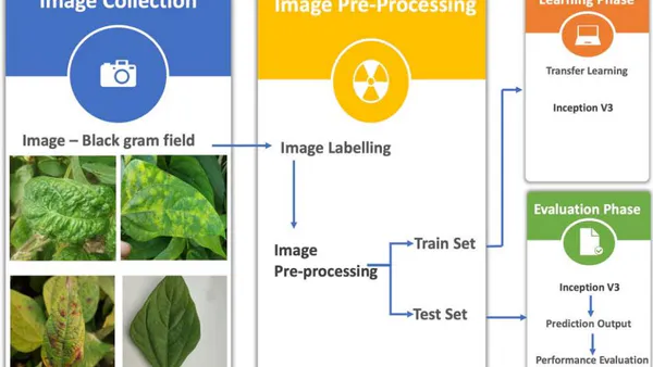
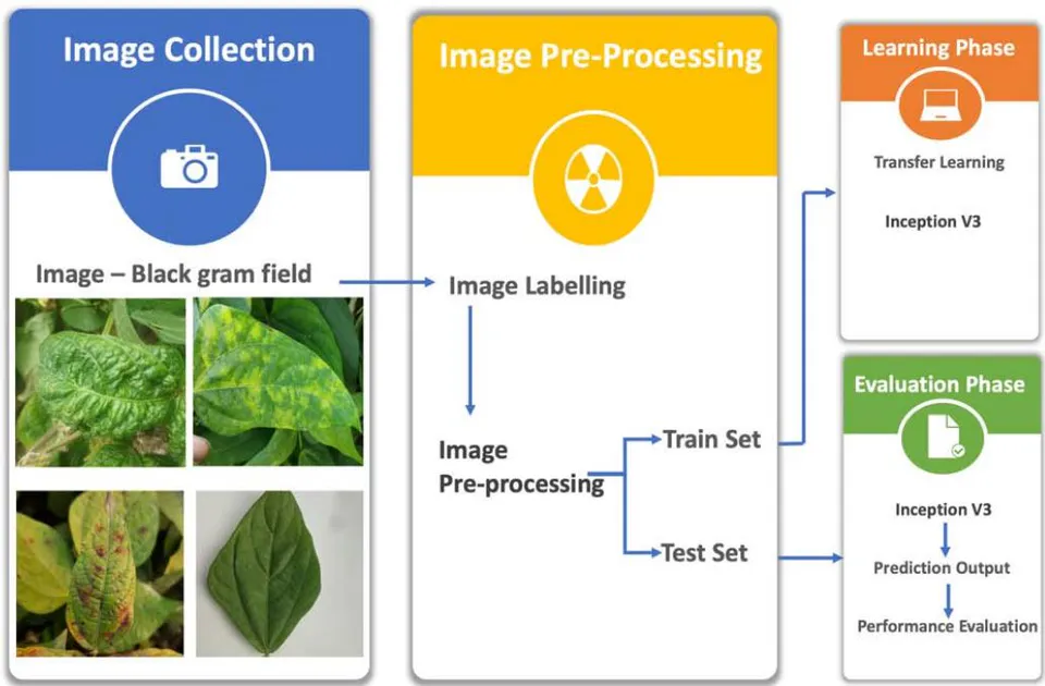
In this study, the work was carried out initially with a survey and collection of samples, application of advanced V3 inception model progresses such as preprocessing of images, learning phase and evaluation phase for diagnosis of foliar diseases in black gram.

a) Survey and Collection of Disease Images

Depending upon the disease prevalence, consecutively cultivating of same varieties of rice fallow black gram, this location was selected for these studies. During Kharif 2022, a vast survey was conducted on rice fallow black gram cultivated fields in four different blocks, such as Aranthangi, Gandarvakottai, Pudukkottai and Thiruvarankulam of Pudukkottai district in Tamil Nadu (Table 1).

S. No.	Survey Conducted Villages	Geo Co- ordinates	Name of the Blocks	Name of the District	Cultivars
1.	Vannarapatti	10.52;78.96	Pudukkottai
2.	Vannarapatti	10.52;78.96	Pudukkottai
3.	Adanakottai	10.53;78.96	Pudukkottai
4.	Adanakottai	10.53;78.97	Pudukkottai
5.	S.Solagampatti	10.59;79.02	Gandarvakottai
6.	S.Solagampatti	10.59;79.01	Gandarvakottai
7.	S.Solagampatti	10.59;79.01	Gandarvakottai
8.	S.Solagampatti	10.59;79.01	Gandarvakottai
9.	Puthunagar	10.62;79.04	Gandarvakottai
10.	Puthunagar	10.62;79.04	Gandarvakottai
11.	Puthunagar	10.43;78.98	Gandarvakottai
12.	Puthunagar	10.43;78.97	Gandarvakottai	Pudukkottai	VBN8, VBN10 & VBN11
13.	Puthunagar	10.42;78.97	Gandarvakottai
14.	Vellalaviduthi	10.51; 79.07	Gandarvakottai
15.	Mankkottai	10.35; 78.95	Thiruvarankulam
16.	Mankkottai	10.35; 78.91	Thiruvarankulam
17.	Kothakottai	10.34;78.91	Thiruvarankulam
18.	Dhatchinapura m	10.34; 78.91	Thiruvarankulam
19.	Pappanpatti	10.37; 78.91	Thiruvarankulam
20.	NPRC, Vamabn	10.36; 78.92	Thiruvarankulam
21.	Ambalapuram	10.19; 79.13	Aranthangi
22.	Sengarai,	10.11; 78.93	Aranthangi
23.	M. S. K. Veedu	10.22; 78.90	Aranthangi
24.	Kunnakkurumb i,	10.21; 78.97	Aranthangi
25.	Ramasamipura m	10.23; 79.13	Aranthangi
26.	Mangalanadu	10.20; 79.14	Aranthangi
27.	Kallaakottai	10.50; 79.08	Aranthangi

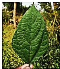
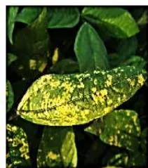
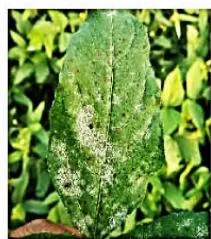
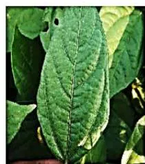
The diseases (anthracnose, powdery mildew, leaf crinkle, yellow mosaic) infected and additionally healthy leaf sample images were captured by a camera (SONY Alpha ILCE-6100Y APS-C) in cultivars of VBN8, VBN10, and VBN11 during sunlight of morning 6.00 to 10.00 am. Totally, 27376 images were collected at 24.2 Mega Pixels (Each one), which comprised disease images such as anthracnose (4225 Nos.), leaf crinkle (6354 Nos.), powdery mildew (6120 Nos.), yellow mosaic (4211 Nos.) and healthy (6466 Nos.). Furthermore, these images were classified by the ratio (80:20) several training sets and several test sets on each and every disease and accompanied by typical symptoms [19], and were described in Table 2.

Images Classificatio n (Diseases)	No. of Using Sets of Images		Total No. of using Sets	Typical Symptoms
	Training Set	Test Set
Anthracnose	3,380	845	4,225	Circular, black, sunken spots with a dark center and bright red-orange margins on leaves [20].
Leaf crinkle	5,084	1,270	6,354	The youngest leaves as chlorosis around some lateral veins and branches near the margin. The leaves show curling of the margin downwards.Some of the leaves show twisting. The veins show reddish-brown discoloration on the under surface which also extends to the petiole [21].
Powdery Mildew	4,896	1,224	6,120	White powdery patches appear on leaves and other green parts which later become dull-colored. These patches gradually increase in size and become circular covering the lower surface completely [22].
Yellow Mosaic	3,201	1,010	4211	Initially, mild scattered yellow spots appear on young leaves and show irregular yellow and green patches alternating with each other. Spots gradually increase in size and ultimately some leaves turn completely yellow. Infected leaves also show necrotic symptoms [23].
Healthy	4,801	1,665	6466	Uninfected
Total No. of images used	21,362	6,014	27,376

b) Image Pre-Processing

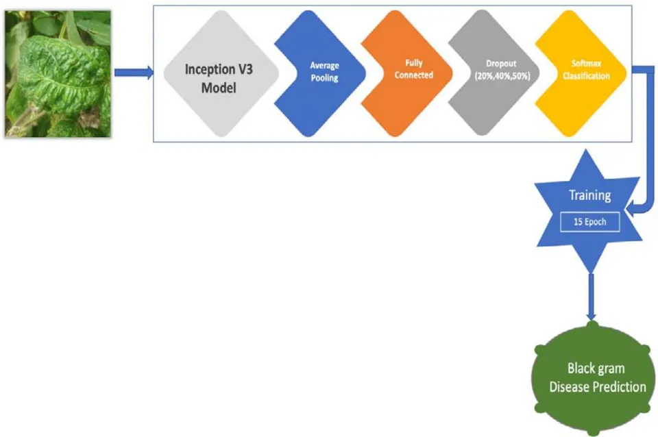
In our experiments, image pre-processing and CNN algorithms, as shown in Figure 1, were implemented using Anaconda 3(Python 3) and the Keras library. The experimental hardware environment includes a Mac Pro with $1.4\mathrm{GHz}$ Quad-Core Intel Core i5. The symptoms-based classified images were further used in this pre-processing. The images were preprocessed using Python programming language with image width, height $150\times 150$ with images $256\times 256$ pixels. Images were trained using the inception V3 model. Images were divided into $80\mathrm{\%}$ training and $20\mathrm{\%}$ testing. In each step, there were different numbers of batches, and each batch contained about 32 images. Data augmentation such as flip, rotation, and zoom were used to create an anomaly dataset for training the model and to detect anomalies. The background noise for images was zoomed out to remove the unnecessary features and to overcome the dropouts. Further, the convolution layers were used to make clarification and diagnosis of diseases with similarity scores and dissimilarities.

c) Application of Convolution Layers

In this layer, the filters or kernels were used to extract the features from the black gram images by moving the kernel over the images, and with the features, feature maps were created. Backpropagation techniques were used with filters and weights. In this layer, the number of parameters was reduced to maintain the network efficiency.

i. Batch Normalization Layers

In this layer data were broken down into mini batches during normalization, to reduce the complexity of the system. In this layer the speed-up process was initiated for training deep neural network features $z$ is remeasured with the equation

Where

• = very small positive number
• = A verage of mini batch mean
• = Mini batch variance

The value of $z$ in the first layer is calculated according to the equation

where

$x=$ the value of input features

To scale and shift the normalized input $\gamma$ and $\beta$ are added, learning using the network parameters through equation

ii. Activation Layers

In this layer, the activation function was used to speed up the arithmetic operation without exploiting the problems. Rectified Linear Unit (ReLU) was used as the basic activation function $\mathbf{z}$ using a mathematical model

The final activation function was used as the output for the last dense layer. The prediction probabilities were 0, 1, 2, 3, 4 for multiple classifications. The softmax function was used for the decimal probabilities of each class. It was calculated from output i with the equation

where $z(i)=$ the output of the i dimension

$\mathsf{m}=$ number of dimensions with respect to the number of classes

The class with the highest probability, while predicting by the method was as described below

iii. Pooling Layers

In these layers, the dimension of feature maps was reduced, selecting the important features created by the convolution layers. There were two poolings: average and maximum pooling. In our model, average pooling, which takes the average value of each feature map, was used.

iv. Fully Connected Layers

In these layers, there were neurons and the last layer of the neural network. With the input, the final output of the pooling or convolution layers is turned into

single vector by means of the flattened layer. The ediction was done using weights, and the final obabilities were given by the dense layer. The number parts in the last dense layer which corresponds to the number of classes.

v. Dropout layer

This layer was used to regularize the neural network and to avoid overfitting by deleting the portion of incoming neurons and their connection.

d) Functions and Optimizations

i. Loss function

This was also called as cost function. The cross-entropy was to find the loss between actual output $y$ and the expected output $\hat{y}$. Cross entropy for multiple classifications was calculated using the equation

ii. Optimization Function

The optimization function was used to reduce the loss function; the Adam optimizer was used in this model. Weights were learned adaptively by Adam Optimizer.

e) Assessment and Evaluation

i. Application of Inception V3 models

In the research paper, Inception V3 was used for pre-training the models. Inception V3 was an additional design for CNN developed by Google. Inception starts with a sparse structure, increases the network depth and width, and clusters the spare data into a dense structure to enhance the model accuracy [26].

Transfer the learning of plant pathology data to the Inception V3 model pre-trained on ImageNet data to speed up the training process and to improve the model performance; the Inception V3 model has 94 convolution layers, 14 pooling, and dense layers [25]. Transfer of learning, pre-trained CNN model includes feature extraction and fine-tuning to achieve the best results. In this paper, feature extraction was first used to train the new classifier, and the model was fine-tuned. Inception V3 was trained using training parameters (Table 3).

Parameter	Value
Batch Size	32
Dropout	20%, 40%, and 50%
Activation function	ReLU, SoftMax
Optimizer	Adam
CNN Training
Epoch	15
Epoch Learning Rate	0.001

Optimization level for Batch size: ; Dropout: 20, 40 & 50% (Study carried out in this experiment at V3 Inception Model) and Epoch 15 is optimized one (Constant) In the research paper, average pooling, dense layer, and SoftMax were added as the activation function for the last layer. The dropout rate was used to train the model. The next step was determining the learning rate, and Adam was used as an optimizer. The

epochs specified were 15 for the training set. The Inception V3 model consists of 21,768,352 trainable parameters during CNN training. The Inception V3 model used to diagnose black gram diseases is summarized in Table 4.

Type of Layer	Output Shape	Parameters
Input	(224, 224, 3)	0
Sequential	(224, 224, 3)	0
Functional (Inception V3)	(5, 5, 192)	393216
Average Pooling	(5, 5, 1280)	0
Dropout	(5, 5, 1280)	0
Dense	(0,3)	512
Total parameters	21,802,784
Trainable parameters	21,768,352
Non-trainable parameters	34,432

CNN has numerous parameters, so there was a possibility of overfitting issues, which can be solved through the dropout procedure. Dropout was a method of randomly disconnecting that can separate connections across different nodes and had a 1-p dropout probability. The dropout layer increases the algorithm's robustness while reducing the number of model parameters. The random inactivation layer enhances the robustness of the network structure and helps to prevent overfitting in the model [26]. Dropout has recently been utilized to reduce overfitting in deep neural networks. Dropout disabled certain neurons in each layer during each epoch, and the remaining neurons were used for forward and backward propagations. As a result, the active neurons were motivated to extract the needed features independently and successfully without the assistance of inactive ones. In this research, dropout rates were 20 percent, 40 percent and 50 percent were studied. Assessment indicators used for the classification of disease diagnosis were accuracy and confusion matrix for comparing models when training and testing the image dataset used. The confusion matrix is a table that shows the classification model performance on the test image set by matching the actual output and expected outputs to identify the correct disease diagnosis. The accuracy is the percentage of valid predictions from the forecast made as per the equation listed below and expressed in percentage.

III. EXPERIMENTAL RESULTS

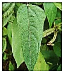
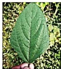
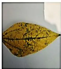
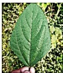
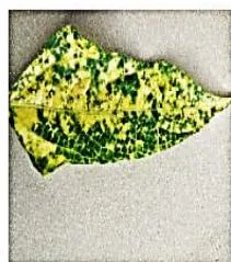
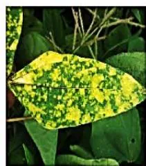
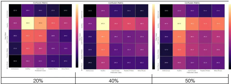
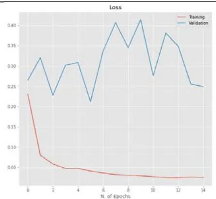
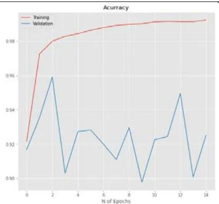
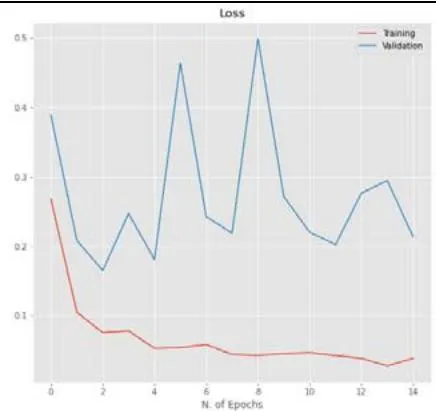
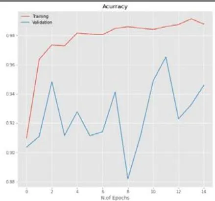
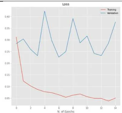
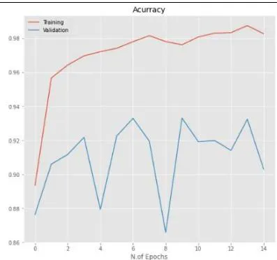
CNN model mentioned in Section 2.5 is trained using the parameters in Table 3 with dropout ratios. The model was compared with accuracy and loss while training and testing, as listed in Table 5. From the table, Inception V3's 20 percent dropout rate was the best model when compared with the 40 percent. The percentage the accuracy of the 20 percent dropout was 99.22 percent, and the loss was 0.0249. The actual and predicted result using CNN is shown in Figure 3. The confusion matrix for the model used by different dropouts is depicted in Figure 4. The changes both in the accuracy and loss of the models used in 20 percent, 40 percent, and 50 percent dropouts were shown in Figure 5. Furthermore, the results suggested that models used in the various study dropouts had an excellent ability to discriminate against black gram diseases. Therefore, based on this empirical analysis, we concluded that the models used in different study dropouts were effective in identifying black gram diseases. This study can be extended for the diagnosis of other plant diseases.

Actual: Healthy Predicted:Leaf Crinkle

Actual: Healthy Predicted: Healthy

Actual: Yellow Mosaic Predicted: Yellow Mosaic

Actual: Healthy Predicted:Healthy

Actual: Powdery Mildew Predicted: Powdery Mildew

Actual: Healthy Predicted: Healthy

Actual: Healthy Predicted: Healthy

Actual: Yellow Mosaic Predicted: Yellow Mosaic Figure 3: The actual and predicted result using CNN

Drop Out (%)	Train		Test
	Accuracy (%)	Loss	Accuracy (%)	Loss
20	99.22	0.0249	92.51	0.2491
40	98.77	0.0384	94.60	0.2132
50	98.27	0.0506	90.32	0.3762

Figure 4: Confusion matrix of black gram leaf disease for Inception V3 model with $20\mathrm{\%}$, $40\mathrm{\%}$, and $50\mathrm{\%}$ dropout values

20%

40%

50% Figure 5: The relationship between accuracy and loss with the number of epochs for the image dataset for the Inception V3 model with $20\mathrm{\%}$, $40\mathrm{\%}$, and $50\mathrm{\%}$ dropout values.

IV. DISCUSSION

The Inception V3 model was employed in this study to diagnose foliar diseases in black gram. Relevant literature was reviewed, and the performance of the Inception V3 model was compared with existing methods. The resulting accuracy obtained is highlighted in Table 6. Deep learning models such as DenseNet, ResNet, and GoogleNet were used to detect tomato diseases [29-33]. The results obtained using these models ranged between 91 percent to 97 percent accuracy. From the proposed model, the obtained accuracy was higher at 99.22 percent. Hence, it was evident that this model had significant improvement compared to other models, as shown in Table 6.

S. No.	Author (s)	Method	Image Number	Image Source	Accuracy (%)
1.	Agarwal et al. (2020) [25]	CNN network	17,500	Plant Village	91.20
2.	Prajwala Tm et al. (2018) [26]	LeNet based CNN	18,160	Plant Village	95
3.	Widiyanto et al. (2019) [24]	CNN model	5000	Plant Village	96.60
4.	Keke Zhang et al. (2018) [23]	ResNet	5550	Plant Village	97.28
5.	Proposed model	Inception V3	27376	TNAU field	99.22

V. CONCLUSIONS

Detection and diagnosis of plant diseases at their earlier stages play a superior role in disease management in crop protection. Keeping this strategy, this work was framed and carried out using deep learning algorithms to diagnose foliar diseases in black gram. This work entirely depends on deep neural networks and their efficacy in image processing, assessment of accuracy, and evaluation. Inception V3 models were used to retrain the transfer learning. The last layer of the models is removed and replaced with average pooling, fully connected, and softmax, respectively. Different dropout rates were used, such as 20 percent, 40 percent, and 50 percent. The experimental results showed that a high degree of accuracy was obtained in diagnosing diseases in black gram using deep learning algorithms. It was reported that a high degree of accuracy of 99.22 percent and a reported loss of 0.0249 percent were obtained in this study by using deep learning algorithms. Further, the image dataset can be expanded for more accurate and high-end results. Under field conditions, manual visualization can lead to errors in plant disease diagnosis due to abiotic factors such as light intensity, weather, and manual handling errors. However, with this approach, these factors have no effect from the field to the laboratory. So, future investigation of this research will focus on diagnosing other plant diseases.

ACKNOWLEDGMENT

I want to express my deepest gratitude to the authors of Saeed, A.; Abdel-Aziz, A.A.; Mossad, A.; Abdelhamid, M.A.; Alkhaled, A.Y.; Mayhoub, M for their valuable research inputs in the paper Smart Detection of Tomato Leaf Diseases Using Transfer Learning-Based Convolutional Neural Networks.