## I. BACKGROUND The reliability of hard drives remains a vital concern across various sectors with particular significance in cloud services and enterprise-level data management where the integrity and availability of data are paramount. As businesses increasingly rely on data-driven decision-making, the cost of data loss or system downtime due to hard drive failures is substantial and impact operational efficiency, customer satisfaction, and financial performance. At enterprise-Level data centers, hard drives often operate under high-demand conditions, which can accelerate wear and tear. The data stored in these centers is crucial for operations and often includes transaction histories, client data, and business analytics. The failure of hard drives in such setups not only leads to data loss but also affects the redundancy and resilience of the entire data system. Regular monitoring and predictive maintenance facilitated by machine learning can significantly reduce the risk of such occurrences (Wang et al., 2018). Cloud services rely on data centers spread across multiple locations, where data is stored redundantly on numerous hard drives. Cloud providers must ensure high reliability to maintain service level agreements and customer trust. Predicting hard drive failure within these systems is not just a maintenance task but a critical operation that directly influences service quality and business continuity (Barroso et al., 2016). The implementation of predictive maintenance strategies for hard drives using machine learning algorithms has been shown to reduce unexpected downtime significantly. By analyzing SMART (Self-Monitoring, Analysis, and Reporting Technology) data, models can predict failures before they happen, allowing for timely replacements and repairs, thus minimizing downtime and reducing maintenance costs (Vishwanath and Nagappan, 2016). The study by Pinheiro, Weber and Barroso (2007) analyse a large population of disk drives and identifies common failure trends and indicators using statistical analysis to explore various SMART attributes. Critical indicators of failures were identified, but the study primarily focused on descriptive statistics rather than predictive modeling. Botezatu et al. (2016) developed prediction system for disk replacements in data centers to improve reliability. Machine learning models are employed to forecast when disks will need to be replaced, using a combination of real-time and historical SMART data. Achieved high accuracy in predictions; however, the study focused majorly on replacement timing rather than immediate failure detection. Hamerly and Elkan (2021) applied Bayesian methods to predict disk drive failures. The study uses Bayesian networks to model the probability of drive failures based on SMART attributes. In comparison, their method provides a probabilistic approach to prediction which is insightful for uncertainty estimation but did not align with the needs for precise regression predictions. With existing works mostly with statistical analysis and machine learning classification, there is a potential gap in exploring more comprehensive array of regression techniques, including advanced polynomial and nonlinear regression models that might capture more complex relationships in the data. ### Research Question Which regression model provides the best performance in predicting hard drive failures based on the identified predictors? ## II. LITERATURE REVIEW Predicting failures is vital aspect of maintenance strategies which target is to prevent unplanned downtimes (Leukel, Gonzalez and Riekert, 2021). Concerning hard drive, while it is a resource that has been commonly adopted as a major storage device due to its cheap price and stability, rapid expansion of data storage systems expose it to failure (Gers, Schmidhuber and Cummins, 2000; Manousakis et al. 2016). According to Bairavasundaram et al. (2008), as disk capacity increases, chances of errors and data loss becomes high. By all standard, failure is costly and it is necessary they are detected or predicted (Murray, Hughes and Kreutz-Delgallo, 2005). Historical dataset based on SMART convention has aided utilization of machine learning in detection and prediction framework. Self-Monitoring and Reporting Technology (SMART) system uses attributes retrieved when hard drive perform and also during off-line tests to fix a failure prediction flag (Murray, Hughes and Kreutz-Delgallo, 2005). In most case, the SMART attributes in hard drive historical data is enormous while possessing target variable that enable classification (failure detection: yes or no) and regression (temporal prediction). Even when the data is primarily available and embedded with continuous and temporal attributes, most research in this domain focuses more on classification. Perhaps as it is good to detect the occurrence of failure, it is essential to predict when it is likely going to happen. A quick and random search on Google Scholar produced predictions based on classification (Table 1) Table 1: Existing works on Hard Drive Prediction <table><tr><td>Author</td><td>Problem Formation</td><td>Machine Learning Techniques</td></tr><tr><td>Aussen et al. 2017</td><td>Classification</td><td>SVM, Random Forest and Gradient Boosting</td></tr><tr><td>Shen et al. 2018</td><td>Classification</td><td>Random Forest</td></tr><tr><td>Garcia et al. 2018</td><td>Classification</td><td>Naïve Baye, SVM and Neural Network</td></tr><tr><td>Amran et al. 2021</td><td>Classification</td><td>Optimal Survival Trees and Optimal Classification Trees</td></tr><tr><td>Chhetri et al. 2022</td><td>Classification</td><td>Relational Graph Convolutional Neural Network</td></tr><tr><td>Ahmed and Green 2022</td><td>Classification</td><td>Random Forest, GBM and Logistic Regression</td></tr><tr><td>Wang et al. 2023</td><td>Classification</td><td>Naïve Baye, Random Forest, SVM, Gradient Boosted Decision Tree, CNN and LSTM</td></tr><tr><td>Zhang et al. 2023</td><td>Classification</td><td>SVM, Random Forest, Gradient Boosted Decision Tree and LSTM</td></tr><tr><td>Gour and Waoo 2023</td><td>Classification</td><td>LightGBM, Random Forest, Decision Tree, Deep Neural Network, Convolutional Neural Network and Recurrent Neural Network</td></tr></table> Unlike many other investigations adoption classification problem, Anantharaman, Qiao and Jadav (2018) uses regression techniques to estimate the remaining useful life of hard disk drives directly. This contrasts with typical predictive models that classify whether a hard disk will fail within a specific timeframe. Random Forest and LSTM were used to analyse SMART attributes with focus of capturing historical temporal patterns that signify deterioration over time. The study evaluates the models based on their Mean Absolute Error (MAE), standard metric for regression tasks. While confidence level of models $(\mathsf{R}^2)$ were not reported in the work, Random Forest model achieved an MAE of 22.66 without a sliding window and 24.08 with a sliding window of size 10. For the LSTM models, the Many-to-One configuration recorded MAEs of 27.62 without a sliding window and 24.81 with it, at the same time the Many-to-Many setup had MAEs of 23.26 and 29.04 for the respective window configurations. Notably, the Piece-wise RUL approach in the Many-to-Many model significantly improved performance, yielding MAEs of 8.15 without a sliding window and 9.31 with a sliding window of size 10. Research by Zufle et al. (2020) applied both classification and regression to the prediction of hard drive failure using random forest machine learning techniques. Just like Anantharaman, Qiao and Jadav (2018), the confidence level metrics were not explicitly presented; the unfiltered data achieved a Mean Absolute Error (MAE) of 10 hours and a Root Mean Square Error (RMSE) of 44.6 hours and the pre-filtered data significantly improved these metrics, with an MAE of 4.5 hours and an RMSE of 12.8 hours. To explore more insights based on temporal and continuous-based predictions, this research will apply four machine learning regression including random forest, decision tree, SVM, Gradient Boosting and Neural Network. ## III. DATASET COLLECTION Based on the view of Ruggiano and Perry (2019), secondary data can be collected and used to address new questions. A suitable and relevant dataset to achieve the study aim and objectives is sourced from Kaggle Hard Drive Test Data (kaggle.com). The dataset originated from BackBlaze and it is based on SMART statistics which makes it readily available for computational handling. 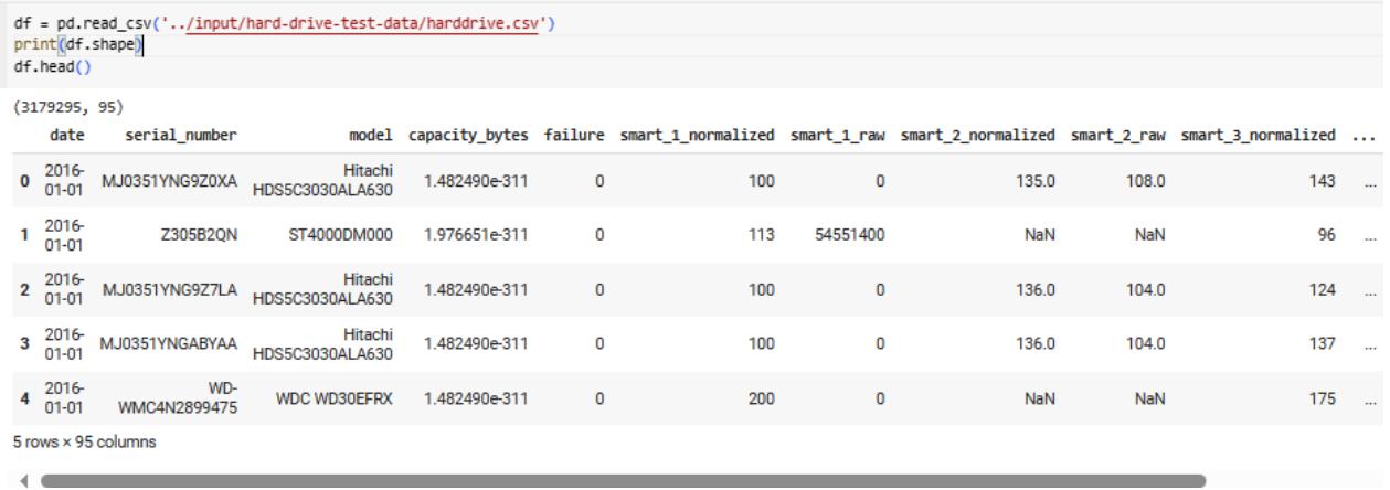 Figure 2: Extract of Data Pre-Processing Figure 1: Extract of Hard Drive Performance Dataset The dataset (Figure 1) contains data related to hard drive diagnostics with various attributes and readings from S.M.A.R.T (Self-Monitoring, Analysis, and Reporting Technology) data. The observation date is measure with attribute named "date". The "serial number" is the unique identifier for each hard drive, while the "model" denotes the model number of the hard drive. The drive's capacity is represented by "capacity_bytes", which is the size of the storage. The attribute "failure" is a binary indicator (0 or 1) where '1' indicates that the hard drive failed on this date. This attribute is used in prediction based on classification as the target variable. The remaining ninety attributes (columns) represent normalized and raw values of different SMART attributes which measure the health and performance of the hard drive. The preprocessing script (Figure 2) cleans the data by removing empty columns, identifies unique drives and models, isolates the subset of data concerning failed hard drives and provides basic counts that help understand the composition of the dataset. {"code_caption":[],"code_content":[{"type":"text","content":"[] df = df.loc[:, -df.isnull().all()] print(df.shape) \n(3179295, 91) \n[] # number of hdd print(\"number of hdd:\", df['serial_number'].value_counts().shape) # number of different types of harddrives print(\"number of different harddrives\", df['model'].value_counts().shape) \nnumber of hdd: (65993,) number of different harddrives (69,) \n[] failed_hdds = df.loc[df==1][\"serial_number\"] len(failed_hdds) \n215 \n[] df = df.loc[df[\"serial_number\"].isin(failed_hdds)] df.shape \n(5498, 91) "}],"code_language":"python"} ## IV. MODEL DEVELOPMENT AND IMPLEMENTATION ### a) Decision Tree Decision Tree is executed using the DecisionTreeRegression function (Figure 3). The function builds a regression tree by recursively splitting the dataset based on feature values to minimize variance within the target variable which ensure each split results in subsets with reduced variance compared to the parent node. The implementation starts by confirming that the dataset can be split further based on the minimum sample size or maximum tree depth; if not, it returns the mean target value of the dataset as a leaf node. The function iterates over all possible splits for each feature, computes the variance reduction for each and selects the split that maximizes this reduction. When the best split is achieved, the dataset is divided and the function is called recursively for each subset until leaf nodes are formed. {"code_caption":[],"code_content":[{"type":"text","content":"Function Decision_Tree_Regression(Data, Depth, Max_Depth, Min_Split_Size) // Input: Data - the dataset for building the regression tree // Depth - the current depth of the tree // Max_Depth - the maximum allowable depth for the tree // Min_Split_Size - the minimum size of the dataset to allow further splits "}],"code_language":"txt"} 1. If Data has fewer rows than Min_Split_Size or Depth equals Max_Depth: 2. Compute and return the mean of the target variable in Data (create a leaf node) 3. Initialize best score to infinity // Used to track the best variance reduction found 4. Initialize best_split to null // Stores the best feature and split point 5. For each feature in Data: 6. For each possible split point within this feature: 7. Split Data into two subsets (Data_Left and Data_Right) based on this split point 8. Calculate the sum of squared residuals from the mean in both subsets 9. Compute the variance reduction as the difference between the variance before and after the split 10. If the variance reduction is greater than best score: 11. Update best_score with this variance reduction 12. Update best_split with this feature and split point 13. If best_split is null: // No valid split was found 14. Compute and return the mean of the target variable in Data (create a leaf node) 15. Use best_split to partition Data into Data_Left and Data_Right 16. Create a node that stores the feature and split point from best_split 17. Recursively apply Decision_Tree_Regression to Data_Left: 18. Left_Child = Decision_Tree_Regression(Data_Left, Depth + 1, Max_Depth, Min_Split_Size) 19. Recursively apply Decision_Tree_Regression to Data_Right: 20. Right_Child = Decision_Tree_Regression(Data_Right, Depth + 1, Max_Depth, Min_Split_Size) 21. Attach Left_Child and Right_Child to the current node as its branches 22. Return the current node // This node now represents the decision at this level of the tree End Function Figure 3: Pseudocode for Implementing Decision Tree The model by the decision tree technique provides a strong alignment between actual and predicted values along the central line but it exhibits noticeable variance and outliers (Figure 4). This indicates that while the Decision Tree will predict hard drive failures using the SMART dataset while its predictions are less stable and accurate with more frequent errors.  Actual vs Predicted Values (Decision Tree) Figure 4: Decision Tree Prediction Outcome ### b) Random Forest The algorithm is implemented by creating an empty list, forests, to store the decision trees (Figure 5). For each tree in the list forest, it generates a bootstrapped sample of the training data. It fits a decision tree regression model using specified parameters like the number of features to consider for each split, the minimum number of samples required to split a node and the maximum depth of each tree. These trees are appended to the forests list. To make predictions, the predict function aggregates predictions from all trees for the test data, averaging their outputs to produce the final prediction. Inputs: data: training dataset n trees: number of trees in the forest n_features: number of features to consider for each split min_samples_split: minimum number of samples required to split a node max_depth: maximum depth of each tree Begin forests $=$ [] for i from 1 to n_trees do $$ bootstrapped_data = bootstrap_sample(data) $$ $$ tree = DecisionTreeRegression(bootstrap_data, n_features, min_samples_split, max_depth) $$ forests.append.tree) end for function predict(test_data) $$ predictions = [] $$ for tree in forests do {"code_caption":[],"code_content":[{"type":"text","content":"predictions.append.tree.predict(test_data))\nend for\nfinal_prediction = average(predictions)\nreturn final_prediction\nend function\nEnd "}],"code_language":"lua"} Figure 5: Pseudocode for Implementing Random Forest 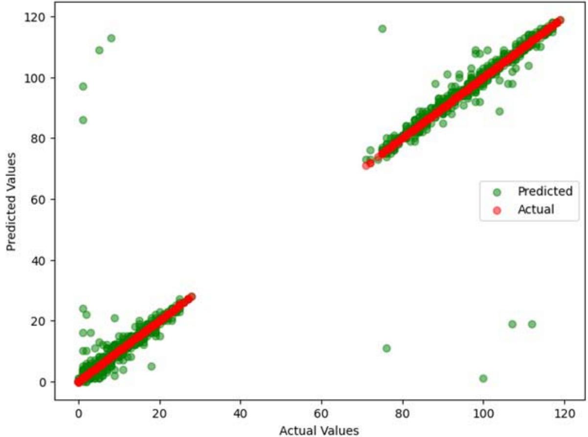The outcome of random forest showed model that is highly effective at predicting hard drive failures using the SMART dataset (Figure 6). However, there are some deviations particularly at higher value ranges and this indicate instances where the model's predictions are less accurate.  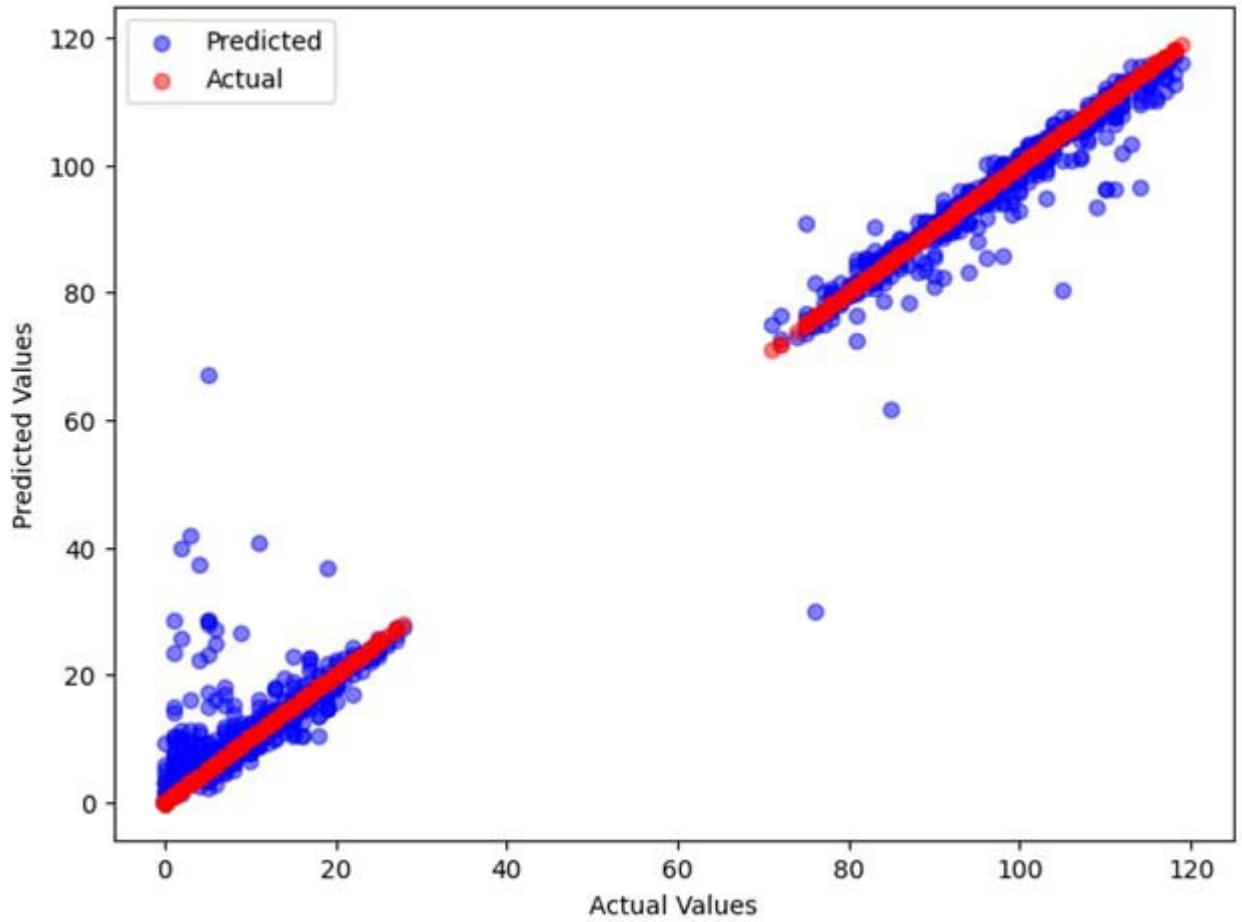Actual vs Predicted Values (Random Forest) Figure 6: Random Forest Prediction Outcome ### c) Support Vector Machine (SVM) From Figure (7.), the implementation begins by initializing the dataset by specifying parameters like epsilon (for error tolerance), the regularization parameter (C), and the kernel type (linear, polynomial, or radial basis function). The kernel function is defined based on the selected kernel type which transforms the input data into a higher-dimensional space to enable separation. For each data point in the training set, the loss function is computed considering the hinge loss for points outside the epsilon margin and at the same time the model parameters are optimized using an algorithm like Sequential Minimal Optimization. The training continues iteratively until convergence criteria are met, after which the final model parameters are saved to enable the SVM to predict hard drive failures on new instances by computing their positions relative to the support vectors and summing the weighted contributions. #### 1. Input: - Data: Dataset containing features and target values - Epsilon: Specifies the epsilon-tube within which no penalty is associated in the training loss function with points predicted within a distance epsilon from the actual value - C: Regularization parameter, which defines the trade-off between achieving a low error on the training data and minimizing model complexity for better generalization - Kernel_Type: Type of kernel function to use (linear, polynomial, radial basis function) 2. Initialize the model parameters (weights and bias) to zero or small random values #### 3. Define the kernel function based on Kernel_Type: instance in the training data: 4. For each instance in the training Data: - Calculate the loss function considering: - Hinge loss for points outside the epsilon margin - Regularization term using C 5. Use an optimization algorithm (e.g., Sequential Minimal Optimization) to: - Select a subset of training instances as support vectors - Optimize the model parameters to minimize the objective function (loss + regularization) 6. Continue iterating over the training set until convergence criteria are met, such as: - No substantial change in the loss function - Reaching a maximum number of iterations 7. Save the model parameters (support vectors, weights, bias) after training is complete Testing: #### 1. Input: - Model: The trained SVM regression model (containing support vectors, weights, bias) - New_Data: New instances for which to predict the target values 2. For each instance in New_Data: - Compute the prediction by applying the kernel function between the new instance and each support vector, scaled by the corresponding weight, and summed with the bias 3. Return the predictions for all instances in New_Data Figure 7: Pseudocode for Implementing SVM The outcome (Figure 8) indicates that the Support Vector Machine (SVM) model struggles with accurately predicting hard drive failures as evidenced by the clustering of predicted values around specific ranges and significant deviations from the actual values.   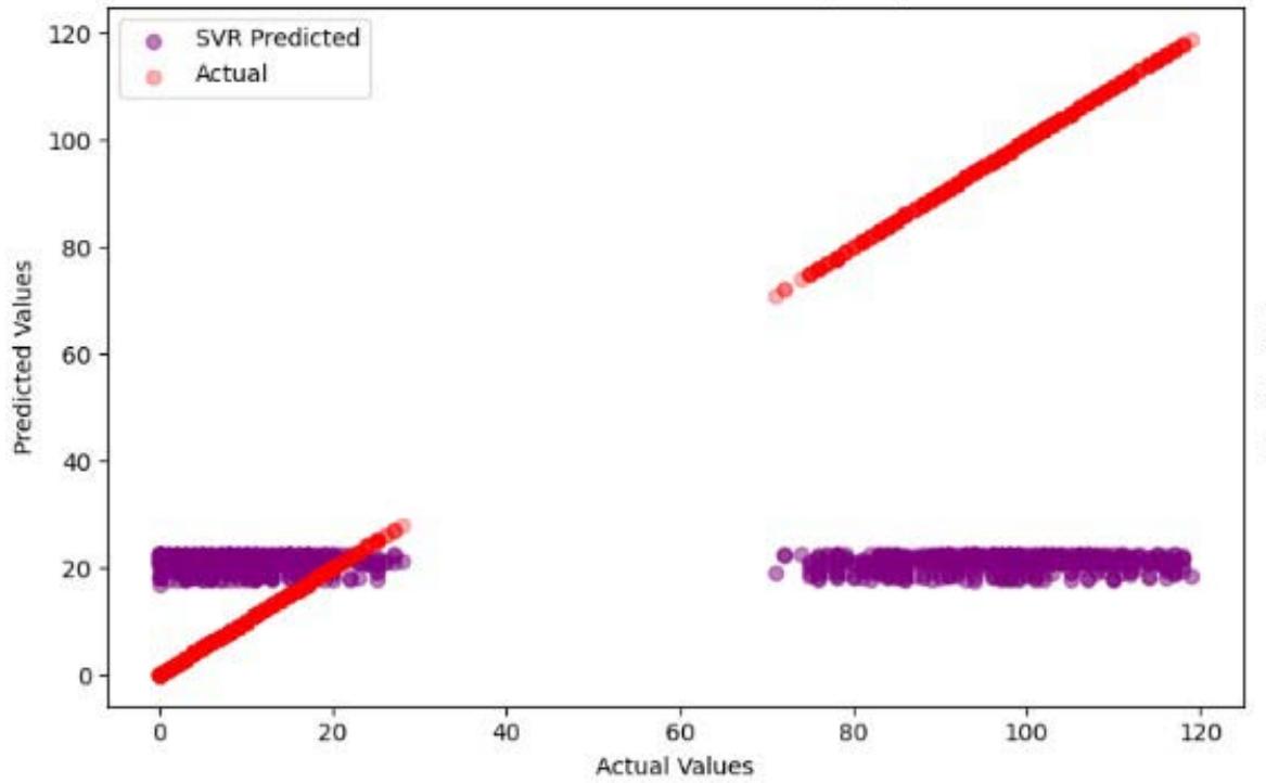Actual vs Predicted Values (SVR) Figure 8: SVM Prediction Outcome ### d) Gradient Boosting The implementation of Gradient Boosting starts with initializing the model, which initially predicts the mean of the target values (Figure 9). For each of the specified number of trees, the model computes the residuals (differences between actual target values and current predictions), which serve as the target for fitting the next tree. Each new tree is trained on these residuals, adhering to constraints like maximum depth and minimum samples required to split. The model is updated by adding the scaled predictions of the new tree to the current model's predictions, iteratively improving accuracy. This process continues until all trees are built, making an ensemble model that makes final predictions on new data by aggregating the contributions of all trees. #### 1. Input: - Data: Dataset containing features and target values - Learning_Rate: Shrinks the contribution of each tree by this factor to improve model robustness - N_Trees: Number of trees to build (iterations) - Max_Depth: Maximum depth of each tree - Min_Samples_Split: Minimum number of samples required to split an internal node #### 2. Initialize: - Model = an initial model which could just predict the mean of the target values of Data 3. For $i = 1$ to $N$ Trees: 4. Compute the residuals (negative gradient of the loss function) for each training instance: - Residuals = actual target values - predictions from the current Model 5. Fit a new tree to the residuals using the feature values with the constraints of Max_Depth and Min_Samples_Split 6. Predict the residuals for the training dataset using this new tree 7. Update the Model by adding the scaled predictions of the new tree: $$ - Model = Model + Learning_Rate * new tree predictions $$ #### 8. Return the final Model Testing: #### 1. Input: - Model: The trained Gradient Boosting model (ensemble of trees) - New_Data: New instances for which to predict the target values 2. Start with the initial prediction (often the mean of the training target values if that was the initialization) 3. For each tree in the Model: 4. Update the prediction for each instance in New_Data: - Prediction $+ =$ Learning_Rate $\star$ tree's prediction on New_Data 5. Return the final predictions for all instances in New_Data Figure 9: Pseudocode for Implementing Gradient Boosting The results (Figure 10) indicate that the Gradient Boosting model produces predictions that align closely with the actual values, as seen by the clustering of prediction dots around the line of equality. However, there is a noticeable dispersion in the predicted values, particularly at the lower and middle ranges. 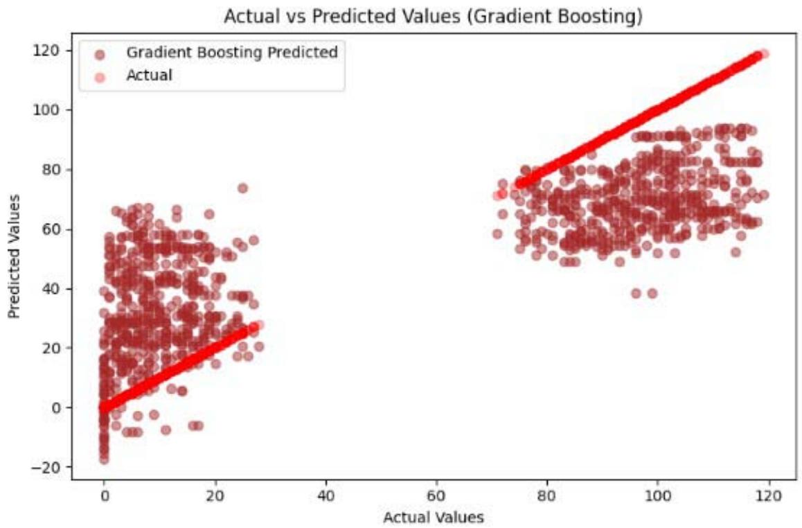 Figure 10: SVM Prediction Outcome ### e) Neural Network The implementation (Figure 11) starts with defining the network's structure and this includes the number of input neurons (corresponding to the dataset features), hidden layers and output neurons. The network is initialized with random weights and biases for each layer. During training, the network processes each training instance by propagating inputs through the layers with the application of activation functions at each hidden layer and computation of the output. The loss function which stands for mean squared error measures the difference between the predicted and actual values while backpropagation is used to update the weights and biases by minimizing this loss. After training, the neural network is tested by passing new data through the trained model to predict hard drive failures, with aggregating predictions for final output. #### 1. Input: - Num_Input Neurons: Number of neurons in the input layer, corresponding to the number of features in the dataset - Hidden_Layers: Number of hidden layers in the network - Neurons_Per_Layer: Array containing the number of neurons in each hidden layer - Output_Neurons: Number of neurons in the output layer #### 2. Structure: - Create a network structure with the specified number of layers and neurons - Initialize weights and biases for each layer randomly #### 3. Return the initialized network with weights and biases #### 1. Input: - Network: Initialized neural network structure with weights and biases - Data: Training dataset features - Labels: Training dataset target values (continuous) - Learning_Rate: Step size for updating the weights - Epochs: Number of times to iterate over the entire training dataset #### 2. Training Process: - For each epoch: 3. For each instance (Input, Target) in (Data, Labels): #### 4. Forward_Propagation: - Compute the output of each layer starting from input to output layer - Use activation functions like ReLU for hidden layers and linear for the output layer #### 5. Compute Loss: - Calculate the mean squared error or another suitable loss function between the predicted and actual values #### 6. Backward_Propagation: - Calculate gradients of the loss function with respect to each weight and bias - Update weights and biases using these gradients and the learning #### Testing: #### 1. Input: - Network: Trained neural network - New_Data: New instances for which to predict the target values #### 2. Prediction Process: - For each instance in New_Data: #### 3. Forward_Propagation: - Compute the output using the trained network starting from the input layer to the output layer #### 4. Collect and return all predictions for New Data Figure 11: Pseudocode for Implementing Neural Network The outcome (Figure 12) shows a significant reduction in both training and validation loss over the epochs, indicating that the neural network is learning and improving its predictions for hard drive failures using the SMART dataset. The close alignment between the training and validation loss curves suggests that the model generalizes well to unseen data, minimizing overfitting and ensuring robust predictive performance.  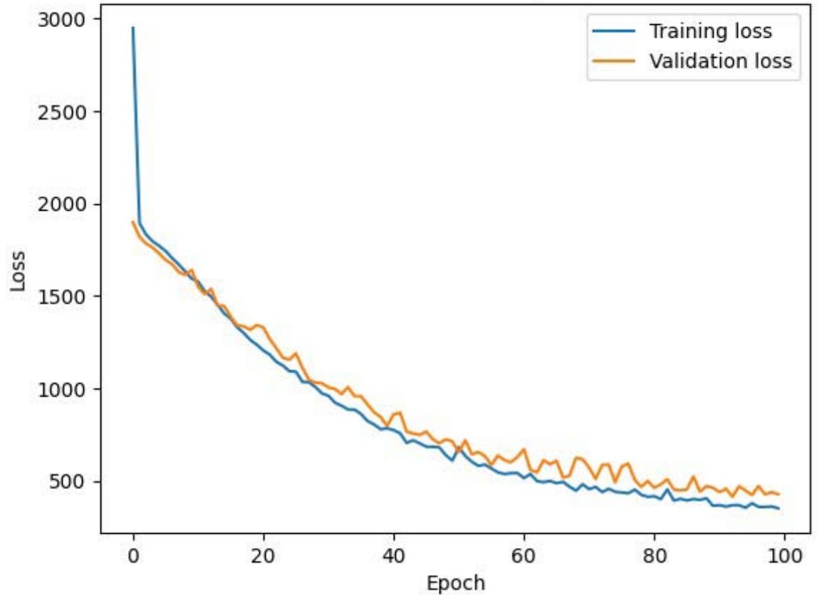Model Loss Over Epochs Figure 12: Neural Network Prediction Outcome ## V. RESULTS AND DISCUSSION For the Decision Tree model (Table 2), the MSE is 71.4943, with an $R^2$ of 0.9642, indicating a high degree of accuracy. The Random Forest model has an MSE of 24.7427 and an $R^2$ of 0.9876, suggesting even better performance. The SVM model shows an MSE of 2888.8623 and an R2 of -0.4465, indicating poor predictive capability. The Gradient Boosting model has an MSE of 823.1132 and an $R^2$ of 0.5879, reflecting moderate accuracy. Lastly, the Neural Network model reports an MSE of 22.6011 and an $R^2$ of 0.7442, which indicates good performance. Table 2: Models Results <table><tr><td>Models</td><td>MSE</td><td>R2</td></tr><tr><td>Decision Tree</td><td>71.4943</td><td>0.9642</td></tr><tr><td>Random Forest</td><td>24.7427</td><td>0.9876</td></tr><tr><td>SVM</td><td>2888.8623</td><td>-0.4465</td></tr><tr><td>Gradient Boosting</td><td>823.1132</td><td>0.5879</td></tr><tr><td>Neural Network</td><td>22.6011</td><td>0.74424</td></tr></table> The Decision Tree model (Figures 13 and 14) exhibits a relatively low MSE of 71.4943, indicating minimal errors in predictions, and a high $R^2$ value of 0.9642, suggesting it explains a large portion of the variance in the target variable effectively. The Random Forest model performs even better, with a significantly lower MSE of 24.7427 and an $R^2$ of 0.9876, indicating excellent explanatory power. This shows that the ensemble approach of combining multiple decision trees improves prediction accuracy and robustness, reducing the impact of overfitting associated with individual trees. 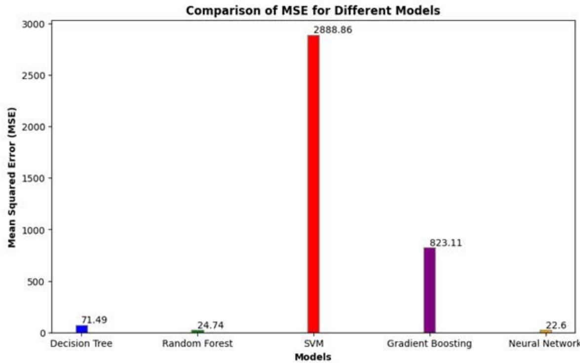 Figure 13: MSE for Selected Models In contrast, the Support Vector Machine (SVM) model performs poorly with a very high MSE of 2888.8623 and a negative $R^2$ value of -0.4465, suggesting it fails to capture the relationship between the features and the target variable and is worse than a simple mean predictor. Gradient Boosting shows moderate performance with an MSE of 823.1132 and an $R^2$ of 0.5879, indicating more prediction errors and less variance explained compared to the Decision Tree and Random Forest models. While powerful, Gradient Boosting may require more fine-tuning or may not be as effective on the study's dataset.  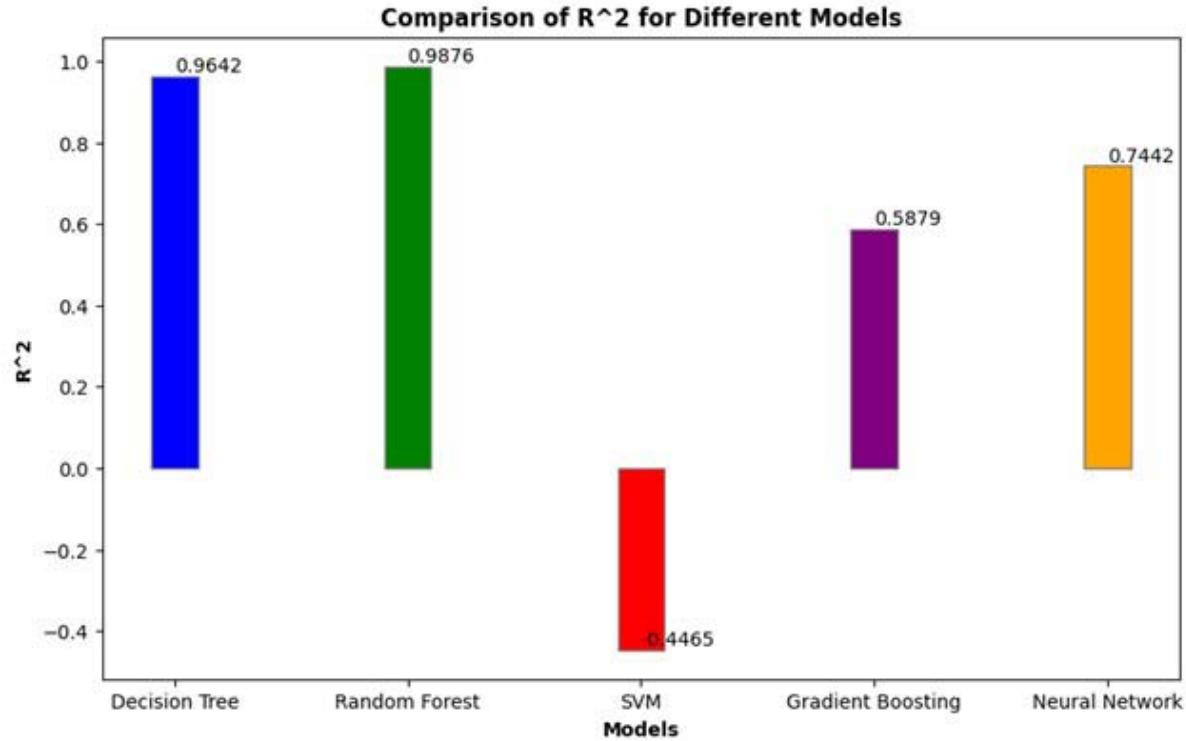Figure 13: $\mathsf{R}^2$ for Selected Models The Neural Network model has the lowest MSE of 22.6011, indicating very accurate predictions with minimal errors, but its $R^2$ value of 0.7442, though high, is not as close to 1 as that of the Random Forest, suggesting some unexplained variance in the data. Neural networks can be very powerful but require substantial data and computational resources, and their performance is highly dependent on the architecture and training process. Overall, the Random Forest perform best with the lowest errors and highest explanatory power. The Neural Network also performs well with very low errors but slightly less explanatory power. The Decision Tree model demonstrates strong performance with good accuracy and explanatory power, while Gradient Boosting has moderate performance. The SVM is not suitable for this task based on the given metrics. ## VI. CONCLUSION, RECOMMENDATION AND LIMITATIONS The research into predictive modeling for hard drive failures using various regression techniques has shown remarkable insights into the efficiency of different models in this domain. The Random Forest and Neural Network models emerged as the best predictors as they demonstrated the highest accuracy and predictive power. The Random Forest model, with an MSE of 24.7427 (minimal predicting error), and an $R^2$ of 0.9876 proved highly effective in capturing the complex relationships within the SMART dataset. Similarly, the Neural Network model exhibited strong predictive capabilities, with an MSE of 22.6011 and an $R^2$ of 0.7442, which indicates robust performance and generalizability. Based on the performance metrics, both random forest and neural network is recommended for predicting hard drive failures. Despite the promising results, a few limitations exist: 1. Model Interpretability: While Random Forest and Decision Tree models offer relatively high interpretability through feature importance, Neural Networks and Gradient Boosting model can be perceived as black-box models. Techniques like SHAP and LIME will help in the interpretability process and overall models explainability. 2. Generalizability: The models were trained and tested on a specific dataset. Their generalizability to other datasets or different types of hard drives may vary. Cross-validation and testing on diverse datasets are important to ensure robustness. 3. Model Maintenance: Predictive models need continuous monitoring and updating to maintain accuracy over time. Changes in hard drive technology and operational conditions necessitate periodic retraining of the models. 4. In conclusion, while the study demonstrates the effectiveness of advanced regression techniques in predicting hard drive failures, addressing these limitations through ongoing research and development is essential for improving model reliability and applicability in real-world scenarios.

Generating HTML Viewer...

References

19 Cites in Article
Jishan Ahmed,Robert Green Ii (2022). Predicting severely imbalanced data disk drive failures with machine learning models.
Maxime Amram,Jack Dunn,Jeremy Toledano,Ying Zhuo (2021). Interpretable predictive maintenance for hard drives.
P Anantharaman,M Qiao,D Jadav (2018). Large Scale Predictive Analytics for Hard Disk Remaining Useful Life Estimation.
Nicolas Aussel,Samuel Jaulin,Guillaume Gandon,Yohan Petetin,Eriza Fazli,Sophie Chabridon (2017). Predictive Models of Hard Drive Failures Based on Operational Data.
Lakshmi Bairavasundaram,Andrea Arpaci-Dusseau,Remzi Arpaci-Dusseau,Garth Goodson,Bianca Schroeder (2008). An analysis of data corruption in the storage stack.
Mirela Botezatu,Ioana Giurgiu,Jasmina Bogojeska,Dorothea Wiesmann (2016). Predicting Disk Replacement towards Reliable Data Centers.
T Chhetri (2022). Knowledge Graph Based Hard Drive Failure Prediction.
M Garcia (2018). Review of techniques for predicting hard drive failure with SMART attributes.
F Gers,J Schmidhuber,F Cummins (2000). Learning to forget: Continual prediction with LSTM.
L Gour,A Waoo (2023). FORENSIC CREDIT CARD FRAUD DETECTION USING DEEP NEURAL NETWORK.
G Hamerly,C Elkan (2001). Bayesian Approaches to Failure Prediction for Disk Drives.
Joerg Leukel,Julian González,Martin Riekert (2021). Adoption of machine learning technology for failure prediction in industrial maintenance: A systematic review.
I Manousakis (2016). Environmental conditions and disk reliability in free-cooled datacenters.
J Murray,G Hughes,K Kreutz-Delgado (2018). Machine Learning Methods for Predicting Failures in Hard Drives: A Multiple-Instance Application.
Nicole Ruggiano,Tam Perry (2019). Conducting secondary analysis of qualitative data: Should we, can we, and how?.
J Shen (2018). Random-forest-based failure prediction for hard disk drive.
Han Wang,Qingfeng Zhuge,Edwin Hsing-Mean Sha,Rui Xu,Yuhong Song (2023). Optimizing Efficiency of Machine Learning Based Hard Disk Failure Prediction by Two-Layer Classification-Based Feature Selection.
Mingyu Zhang,Wenqiang Ge,Ruichun Tang,Peishun Liu (2023). Hard Disk Failure Prediction Based on Blending Ensemble Learning.
M Züfle (2020). To Fail or Not to Fail: Predicting Hard Disk Drive Failure Time Windows.
No ethics committee approval was required for this article type.
Data Availability
Not applicable for this article.
How to Cite This Article
Elizabeth Atekoja. 2026. \u201cPrediction of Hard Drive Failure using Machine Learning\u201d. Global Journal of Computer Science and Technology - D: Neural & AI GJCST-D Volume 24 (GJCST Volume 24 Issue D1).
Explore published articles in an immersive Augmented Reality environment. Our platform converts research papers into interactive 3D books, allowing readers to view and interact with content using AR and VR compatible devices.
Your published article is automatically converted into a realistic 3D book. Flip through pages and read research papers in a more engaging and interactive format.
Our website is actively being updated, and changes may occur frequently. Please clear your browser cache if needed. For feedback or error reporting, please email [email protected]
Thank you for connecting with us. We will respond to you shortly.