I. INTRODUCTION

In general, fracture mechanics has been developed based on the asymptotic expansion of crack tip stress field as well as strain one and displacement one. The elastic-plastic fracture mechanics is based on the crack tip HRR field [12, 22]. Such a HRR field has been originally considered to be characterized by the $J$ -integral in the conventional elastic-plastic fracture mechanics, so called the one-parameter fracture mechanics. The $J$ -integral has been widely used to predict the onset of crack growth as it is a parameter characterizing the singularity of elastic-plastic crack tip field. Nevertheless, numerous experimental studies showed that the fracture toughness $J_{C}$ has a remarkable difference depending on the geometry and the loading mode. Furthermore, it has been established that the elastic-plastic crack tip field could not be characterized efficiently only by the $J$ -integral according to many numerical studies, leading to the emergency of two-parameter elastic-plastic fracture mechanics. The two-parameter elastic-plastic fracture mechanics includes the $J - A_{2}$ approach [5, 30] and the $J - Q$ theory [16, 17]. The $J - A_{2}$ approach is based on the strict mathematical formulation while the $J - Q$ theory belongs to the empirical theory proposed by the numerical studies. The first parameter $J$ represents the singularity of elastic-plastic crack tip field whereas the second one, so called the constraint parameter, reflects the constraint effect of elastic-plastic crack tip field.

It is of great importance to calculate the $J$ -integral as well as $A_{2}$ or $Q$ for the assessment of safety of cracked structure by using the fracture mechanics. In general, numerical method like the finite element method has been widely used for the evaluation of $J$ -integral as well as $A_{2}$ or $Q$ as their analytical formulae could not be specified in most cases. The conventional FEM requires very fine mesh matched with a crack near the crack tip for the reasonable accuracy of solutions, leading to a large number of finite elements and remeshing concerning with the crack propagation.

The extended finite element method (XFEM) is one of the attractive methods for the numerical fracture mechanics since it does not need to use the finer FE mesh near the crack tip and the remeshing as the crack propagates [2, 15]. The main idea of the XFEM is the addition of appropriate functions considering the displacement discontinuity on the crack faces and the displacement singularity due to the crack into the standard FE approximate base on the basis of the partition unity method (PUM), leading to the possibility of employment of the FE mesh mismatched with the crack geometry and the improvement of numerical accuracy for the crack analysis.

The linear elastic fracture mechanics has been primarily concerned with the XFEM. For the elastic crack, four enrichment functions have been based on the asymptotic expansion of displacement near the crack tip considering the only the singular term [2, 15]. Even though some authors suggested the enrichment functions regarding the higher terms as well as the singular term in the asymptotic expansion of displacement field near the crack tip, the effect of enrichment functions considering the higher terms was not been clarified [7, 28, 29]. Moreover, increasing the number of the enrichment function can cause the grown up of the degree of freedom, leading to the expensive cost in computation.

In recent years, although the XFEM has made a leaping progress and increasing interest is being shown in the fracture mechanics, previous investigations of the XFEM have dealt almost exclusively with the linear elastic fracture mechanics and some researchers have studied about the elastic-plastic crack [8, 31-35].

For the elastic-plastic crack, 6 crack tip enrichment functions suggested in [6, 21] are based on the HRR singular field. As mentioned above, the introduction of constraint parameter $A_{2}$ or $Q$ makes it possible to get the more realistic safety assessment of the cracked structure on the basis of the fracture mechanics. Therefore, it is of essential importance to establish the XFEM applied to the elastic-plastic fracture mechanics taking account for the constraint effect. Nevertheless, very little is known about the XFEM on the elastic-plastic constraint effect.

In this paper, a family of the crack tip enrichment function was studied for the XFEM of the 2D elastic-plastic crack based on the $J - Q$ theory.

The contents of this paper are as follows. Section 2 gives a brief description of the $J - Q$ theory and the MBL model for modeling cracks. Section 3 describes briefly the XFEM applied to the fracture mechanics. Section 4 explains the crack tip enrichment functions considering the constraint effect and section 5 considers ANSYS implementation of our model. Numerical results for the MBL model and the two types of specimens are presented in section 6. A few concluding remarks are mentioned in section 7.

II. $J - Q$ THEORY AND THE MBL MODEL

a) $J - Q$ Theory

The $J - Q$ theory assumes that the material follows the Ramberg-Osgood constitutive relation as

$$ \frac{\varepsilon}{\varepsilon_0} = \frac{\sigma}{\sigma_0} + \alpha \left(\frac{\sigma}{\sigma_0}\right)^n $$

where, $n$ denotes the strain hardening exponent, $\alpha$ the material coefficient, $\sigma_0$ the yielding stress, $\varepsilon_0$ the reference strain and $E$ the Young's modulus.

Within a infinitesimal strain theory, the stress field near the mode-I crack tip can be expressed as

$$ \frac {\sigma_ {i j}}{\sigma_ {0}} = \left(\frac {J}{\alpha \varepsilon_ {0} \sigma_ {0} I _ {n} r}\right) ^ {1 / (n + 1)} \tilde {\sigma} _ {i j} (\theta ; n) + Q \left(\frac {r}{J / \sigma_ {0}}\right) ^ {q} \hat {\sigma} _ {i j} (\theta ; n) \tag {2} $$

where, $r$ and $\theta$ are the components in the polar coordinate system with a origin of crack tip and $I_{n}$ is a constant which depends only on the hardening exponent $n$ [16, 17].

In Eqs (2), the first term in the right hand is the well-known HRR field and the second one represents the non-singular term with the amplitude of non-dimensional $Q$ parameter.

The displacement field near the crack tip is expressed as

$$ \frac{u _ {i} - u _ {i} ^ {0}}{\alpha \varepsilon_ {0}} = \left(\frac{J}{\alpha \varepsilon_ {0} \sigma_ {0} I _ {n}}\right) ^ {n / (n + 1)} r ^ {1 / (n + 1)} \tilde{u} _ {i} (\theta) + Q \left(\frac{r}{J / \sigma_ {0}}\right) ^ {q} \left(\frac{J}{\alpha \varepsilon_ {0} \sigma_ {0} I _ {n}}\right) ^ {(n - 1) / (n + 1)} r ^ {2 / (n + 1)} \hat{u} _ {i} (\theta) \tag{3} $$

where, $u_{i}^{0}$ denotes the rigid body translation.

Eqs (2) can be rewritten as

$$ \sigma_ {i j} = \left(\sigma_ {i j}\right) _ {H R R} + Q \sigma_ {0} \left(\frac {r}{J / \sigma_ {0}}\right) ^ {q} \hat {\sigma} _ {i j} (\theta ; n) \tag {4} $$

where a parameter $Q$ should be matched numerically.

Alternative expression for Eqs (4) was suggested as a parameter $Q$ depends on the location of matching point [18, 19]. Namely,

$$ \sigma_ {i j} = \left(\sigma_ {i j}\right) _ {Q = 0} + Q \sigma_ {0} \left(\frac {r}{J / \sigma_ {0}}\right) ^ {q} \hat {\sigma} _ {i j} (\theta ; n) \tag {5} $$

Here, $\left(\sigma_{ij}\right)_{Q=0}$ is the reference solution corresponding to $Q = 0$, which can be evaluated by the FEA of the MBL model.

In this paper, we the displacement field as follows, similar to Eqs (5).

$$ u_{i} = \left(u_{i}\right)_{Q=0} + Q f\left(J, \alpha, \varepsilon_{0}, \sigma_{0}, I_{n}\right) r^{2/(n+1)+q} \hat{u}_{i}\left(\theta\right) = \left(u_{i}\right)_{Q= 0} + \left(u_{i}\right)_{Q} $$

b) The MBL Model

In general, the displacement and the stress near the crack tip can be represented as

$$ \left\{ \begin{array}{l} u _ {1} \\u _ {2} \end{array} \right\} = \frac {K _ {I}}{2 \mu} \sqrt {\frac {r}{2 \pi}} \left\{ \begin{array}{l} \cos \frac {\theta}{2} \left(k - 1 + 2 \sin^ {2} \frac {\theta}{2}\right) \\\sin \frac {\theta}{2} \left(k + 1 - 2 \cos^ {2} \frac {\theta}{2}\right) \end{array} \right\} + \frac {T r}{2 (1 + \nu) \mu} \left\{\left(1 - \nu^ {2}\right) \cos \theta \\- (\nu + \nu^ {2}) \sin \theta \end{array} \right\} \tag {7} $$ $$ \left\{ \begin{array}{l} \sigma_{11} \\\sigma_{12} \\\sigma_{22} \end{array} \right\} = \frac{K_{I}}{\sqrt{2\pi r}} \left\{ \begin{array}{l} 1 - \sin\frac{\theta}{2} \sin\frac{3\theta}{2} \\\sin\frac{\theta}{2} \cos\frac{3\theta}{2} \\1 + \sin\frac{\theta}{2} \sin\frac{3\theta}{2} \end{array} \right\} + \left\{ \begin{array}{l} T \\0 \\0 \end{array} \right\} \tag{8} $$

where, $\nu$ is the Poisson ratio, $\mu = E / 2(1 + \nu)$ the shear modulus and the Kolosov constant $k$ is equal to $k = (3 - \nu) / (1 + \nu)$ for the plane stress and $k = 3 - 4\nu$ for the plane strain.

$K_{I}$ is the stress intensity factor (SIF) and $T$ is the so-called $T$ -stress, which is the constraint parameter.

Eqs (7) and Eqs (8) is called the MBL model.

In the boundary layer model, the elastic-plastic analysis is conducted by the finite element method, employing only the first term in the analytical displacement (7) on the circumference surrounding the crack tip with a certain radius of $R$ [14]. The obtained numerical result can be considered approximately as the analytical solution for the crack. This implies that the first term in Eqs (7) can characterize the crack tip singularity sufficiently.

The MBL model applies the second term as well as the first one in Eqs (7) as the boundary condition, which has been widely used for the study of $J - Q$ theory [3]. By using the MBL model, arbitrary $J - Q$ filed can be easily obtained.

III. XFEM FOR THE CRACK MODELING

The XFEM enriches appropriate functions considering the displacement discontinuity on the crack faces and the displacement singularity due to the crack into the standard FE approximation for the crack modeling. Based on the PUM, the XFEM displacement can be approximated as

$$ \mathbf{u}^{h}(\mathbf{x}) = \sum_{i \in I} N_{i}(\mathbf{x}) \mathbf{u}_{0i} + \sum_{j \in J} N_{j}(\mathbf{x}) H(\mathbf{x}) \mathbf{a}_{j} + \sum_{k \in M} N_{k}(\mathbf{x}) \left(\sum_{\alpha} F^{\alpha}(\mathbf{x}) \mathbf{b}_{k}^{\alpha}\right) \tag{9} $$

where $I$ is a set containing all the nodes in the finite element model, $J$ a subset involving nodes enriched by the Heaviside function and $M$ a subset having nodes enriched by the crack tip enrichment functions. A component $N_{i}$ is the shape function of the standard finite element method concerning with a node $i$ and $\mathbf{u}_{0i}$ is a corresponding degree of freedom. Coefficients $\mathbf{a}_j$ and $\mathbf{b}_k^\alpha$ is the degree of freedom related to the Heaviside function and the crack tip enrichment functions, respectively [2, 15].

The Heaviside function $H(\mathbf{x})$ is defined as

$$ H (\mathbf {x}) = \left\{ \begin{array}{l l} - 1 & \phi (\mathbf {x}) < 0 \\ + 1 & \phi (\mathbf {x}) \geq 0 \end{array} \right. \tag {10} $$

where $\phi(x)$ denotes the signed distance function from the crack (usually determined by means of the level set method, LSM).

For the elastic-plastic crack, the enrichment function $F^{\alpha}(\mathbf{x})$ considering only the HRR field is usually chosen as follows [6].

$$ r ^ {\frac{1}{n + 1}} \left\{\sin \frac{\theta}{2}, \cos \frac{\theta}{2}, \sin \frac{\theta}{2} \sin \theta , \cos \frac{\theta}{2} \sin \theta , \sin \frac{\theta}{2} \sin 2 \theta , \cos \frac{\theta}{2} \sin 2 \theta \right\} $$ $$ r ^ {\frac{1}{n + 1}} \left\{ \sin \frac{\theta}{2}, \cos \frac{\theta}{2}, \sin \frac{\theta}{2} \sin \theta , \cos \frac{\theta}{2} \sin \theta , \sin \frac{\theta}{2} \sin 3 \theta , \cos \frac{\theta}{2} \sin 3 \theta \right\} \tag{12} $$ $$ r ^ {\frac{1}{n + 1}} \left\{ \begin{array}{l} \sin \frac{\theta}{2}, \cos \frac{\theta}{2}, \sin \frac{\theta}{2} \sin \theta , \cos \frac{\theta}{2} \sin \theta , \sin \frac{\theta}{2} \sin 2 \theta , \cos \frac{\theta}{2} \sin 2 \theta , \\\sin \frac{\theta}{2} \sin 3 \theta , \cos \frac{\theta}{2} \sin 3 \theta \end{array} \right\} \tag{13} $$

We use Eqs (12) as the HRR enrichment functions.

IV. ENRICHMENT FUNCTIONS FOR THE ELASTIC-PALSTIC CRACK CONDISERING THE CRACK TIP CONSTRAINT EFFECT

Our attention mainly is focused on the determination of enrichment functions for the second term $\left(u_{i}\right)_{Q}$ in Eqs (6) since the enrichment functions for the HRR field has been suggested previously.

As shown from Eqs (6), the displacement is separated about $r$ and $\theta$. Moreover, the angular distribution function does not depend on the material characteristics and the magnitude of $J$ -integral and $Q$ -stress. Thus, the determination of base functions for the angular distribution functions of displacement field at a specific location near the crack tip is a main key for the material considered.

The finite element analysis package WARP3D is used for the computation of the reference solution corresponding to $Q = 0$ as well as another solutions corresponding to different $Q$ -stresses [10].

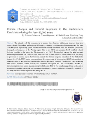
Figure 1 shows the FE mesh for the MBL model.

The analytical displacement near the crack tip (7) is employed on the circumference. Different $J - Q$ fields can be obtained for the fixed $T$ -stress, increasing the stress intensity factor since the $T$ -stress has one-to-one correspondence with the $Q$ -stress.

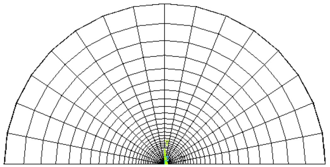Figure 1: FE mesh for the MBL model

The base function for the second term $\left(\boldsymbol{u}_i\right)_Q$ in Eqs (3) is chosen as

$$ r ^ {\frac {2}{n + 1} + t} \left\{\sin \theta , \cos \theta , | \theta + 1 | ^ {\sin | \theta |} \right\} \tag {14} $$

where, $-180^0 < \theta \leq 180^0$

The displacement field at the location of $\frac{r}{J / \sigma_0} = 2$ away from the crack tip is used for the numerical evaluation of accuracy of the chosen base function. A radius of the boundary layer is taken as $R = 1m$ and $n = 10$, $E / \sigma_0 = 500$, $E = 206GPa$ and $\nu = 0.3$. $\frac{T}{\sigma_0} = -0.5$ and 0.5 is applied respectively and the value of $J$ -integral is equal to $50KN/m$ for all cases. Based on Eqs (5), the value of $Q$ is evaluated as -0.52 and 0.24 for $\frac{T}{\sigma_0} = -0.5$ and 0.5, respectively.

Figure 2 shows the displacement curve calculated by using WARP3D for the case of $Q = 0$, -0.52 and 0.24.

Figure 3 and figure 4 shows the comparison of the second term $\left(u_{i}\right)_{Q}$ with the numerical interpolation by the base function of Eqs (14) at the location of $\frac{r}{J / \sigma_0} = 2$ for the case of $Q = 0.24$ and $-0.52$, respectively.

As seen from these figures, the base functions according to Eqs (14) could be the good approximation for the XFEM displacement corresponding to the non-singular terms near the crack tip.

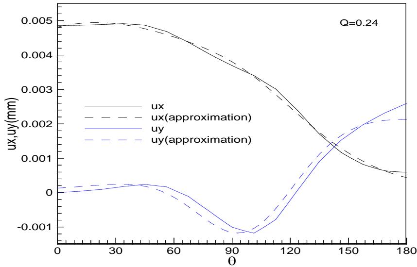Figure 3: Comparison of the second term $\left(u_{i}\right)_{Q}$ with the numerical interpolation by the base function of Eqs (14) at the location of $\frac{r}{J / \sigma_0} = 2$ for the case of $Q = 0.24$

Figure 2: $\left(U_{x}, U_{y} - \theta\right)$ curves for $Q = 0$, -0.52 and 0.24 at the location of $\frac{r}{J / \sigma_0} = 2$

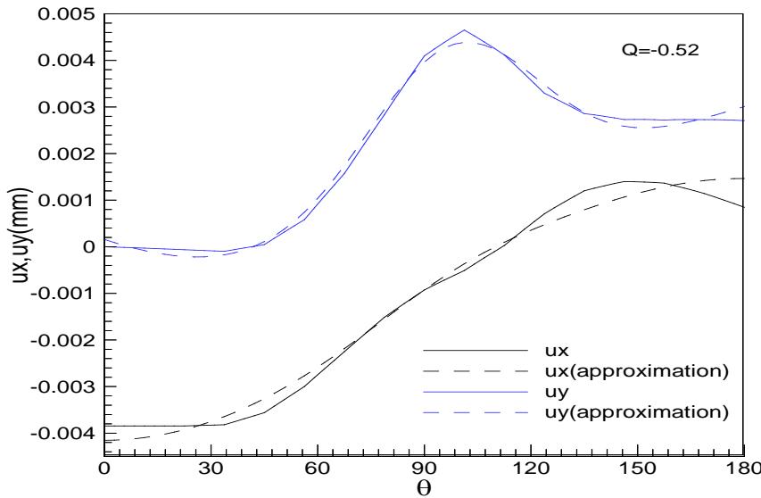Figure 4: Comparison of the second term $\left(u_{i}\right)_{Q}$ with the numerical interpolation by the base function of Eqs (14) at the location of $\frac{r}{J / \sigma_0} = 2$ for the case of $Q = -0.52$

Furthermore, the base function (14) corresponding to the non-singular term should be combined with the one (12) for the HRR singularity, leading to the formulation of base function for the displacement near the crack tip. Namely,

$$ r ^ {\frac {1}{n + 1}} \left\{\sin \frac {\theta}{2}, \cos \frac {\theta}{2}, \sin \frac {\theta}{2} \sin \theta , \cos \frac {\theta}{2} \sin \theta , \sin \frac {\theta}{2} \sin 3 \theta , \cos \frac {\theta}{2} \sin 3 \theta \right\}, \tag {15} $$ $$ r ^ {\frac{2}{n + 1} + q} \left\{\sin \theta , \cos \theta , \left|\theta + 1\right|^{\sin |\theta|} \right\} $$

Figure 5, 6 and figure 7 shows the comparison of the numerical result for the displacement corresponding to $Q = 0.0$, -0.52 and 0.24 with the numerical interpolation by the base function of Eqs (15) at the location of $\frac{r}{J / \sigma_0} = 2$, respectively.

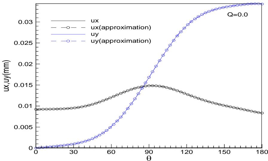Figure 5: Comparison of the numerical result for the displacement corresponding to $Q = 0.0$ with the numerical interpolation by the base function of Eqs (15) at the location of $\frac{r}{J / \sigma_0} = 2$

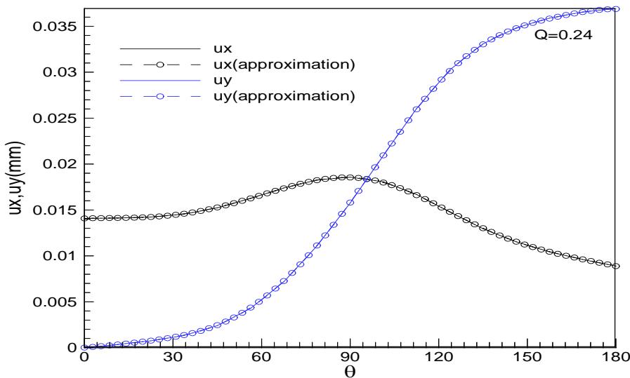Figure 6: Comparison of the numerical result for the displacement corresponding to $Q = 0.24$ with the numerical interpolation by the base function of Eqs (15) at the location of $\frac{r}{J / \sigma_0} = 2$

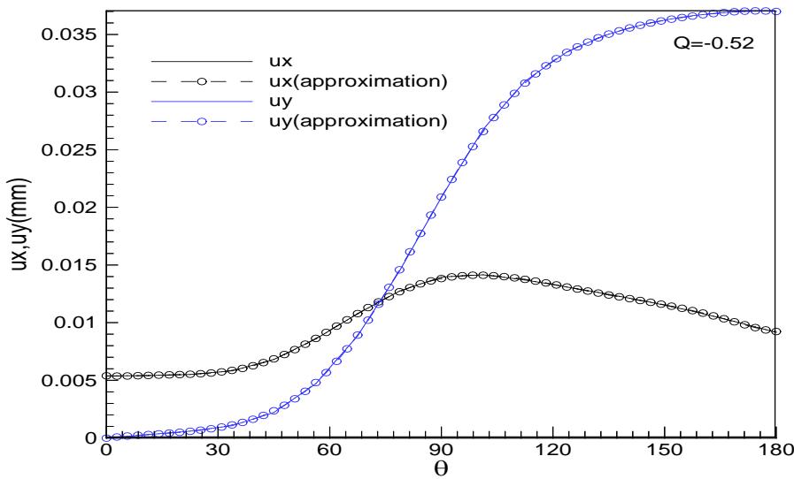Figure 7: Comparison of the numerical result for the displacement corresponding to $Q = -0.52$ with the numerical interpolation by the base function of Eqs (15) at the location of $\frac{r}{J / \sigma_0} = 2$

As shown from these figures, the base functions in Eqs (15) can be a very good approximation for the XFEM applied to the elastic-plastic crack considering the crack tip constraint effect.

V. IMPLEMENTATION OF XFEM APPLIED TO THE ELASTIC-PLASTIC CRACK BY USING ANSYS

The XFEM can not be directly implemented by using the general finite element package as the enriched degrees of freedom are added besides the standard displacement.

In ref [4], Visual C++ has applied for the XFEM implementation. The 2D XFEM package has been developed [20]. The 2D and 3D XFEM has been implemented by using the user-defined element in ABAQUS [9, 25] and Dynaflow has been used for the XFEM implementation [11, 26]. Previous XFEM implementations were aimed to the elastic crack.

In this paper, the 2D elastic-plastic XFEM was implemented based on the UserElem in ANSYS. 4-node quadrilateral elements were used and the 49-point Gauss-Legendre quadrature was employed. The FE mesh was generated by using ANSYS and the elastic-plastic constitutive relation was obtained by calling the ElemGetMat. The UserElem converts the stress at the Gauss point into the nodal stress so that the nodal stress and strain in the user-defined element can be used for the postprocessor, respectively.

The $J$ -integral can be evaluated as follows.

$$ J = \int_ {A} \left(\sigma_ {j i} \frac {\partial u _ {i}}{\partial x _ {1}} \frac {\partial q}{\partial x _ {j}} - W \frac {\partial q}{\partial x _ {1}}\right) d A \tag {16} $$

Here, $x_{i}$ is the components of the local Cartesian coordinates where $x_{1}$ is parallel to the crack faces and the origin locates at the crack tip and $u_{i}$ is the displacement in the $x_{i}$ -direction. $\sigma_{ij}, \varepsilon_{ij}$ and $W$ is the stress, the strain and the strain energy density, respectively. $q$ is a arbitrary smooth function where takes zero on the outer boundary of the integration zone and 1 at the crack tip.

Although ANSYS has the function for calculating the $J$ -integral, it is impossible to apply that function for the user-defined elements. The UserElem writes all the quantities necessary for the evaluation of $J$ -integral into the data file for every load steps. The $J$ -integral could be extracted by the numerical integration of Eqs (16) based on read the data file generated by the UserElem.

VI. NUMERICAL VALIDATION

In this paper, we conducted the numerical simulation for the MBL model, SE(T) and DE(T) in order to validate the effectiveness of the enriched functions suggested by ours taking account for the crack tip constraint effect.

In convenience, we call the enrichment function in Eqs (12) as the HRR enrichment function and the one in Eqs (15) as the $J - Q$ enrichment function. The 1-layer enrichment and the 2-layer one will be selected for the enriched zone. Parameter $q$ will be adopted as in ref [24].

a) The MBL Model

The $T$ -stress depends on the stress intensity factor $K_{I}$ linearly as

$$ T = B \frac{K _ {I}}{\sqrt{\pi a}} $$

where, $B$ is a biaxiality parameter ranging from -0.5 to 2.0 and $a$ is a crack length [1].

The nodes on the boundary layer with a radius $R$ are imposed by the $K - T$ field as

$$ \left\{ \begin{array}{l} u _ {1} \\u _ {2} \end{array} \right\} = \frac {K _ {I}}{2 \mu} \sqrt {\frac {R}{2 \pi}} \left\{ \begin{array}{l} \cos \frac {\theta}{2} \left(k - 1 + 2 \sin^ {2} \frac {\theta}{2}\right) \\\sin \frac {\theta}{2} \left(k + 1 - 2 \cos^ {2} \frac {\theta}{2}\right) \end{array} \right\} + B \frac {K _ {I}}{\sqrt {\pi R}} \frac {R}{2 (1 + \nu) \mu} \left\{ \begin{array}{l} (1 - \nu^ {2}) \cos \theta \\- (\nu + \nu^ {2}) \sin \theta \end{array} \right\} \tag {18} $$

where, a radius of the boundary layer $R$ is taken as a crack length $a$.

The stress intensity factor $K_{I}$ lies between 0 and $300MPa\sqrt{m}$ and a biaxiality parameter $B$ is chosen as -0.5, 0.0 and 1.0, respectively. The material characteristics is assumed as $n = 5$, $E / \sigma_0 = 800$, $E = 206GPa$ and $\nu = 0.3$. The reference solution of $J$ -integral is computed by using WARP3D whose the FE model contains 6119 8-node brick elements.

The element size of the XFEM for the boundary layer model is about $R / 25$. Figure 8 shows the FE mesh for the boundary layer model.

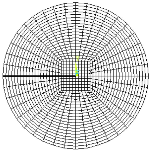Figure 8: FE mesh of the XFEM for the boundary layer model

Figure 9~figure 11 compares the $J$ -integral computed by using WARP3D with the one by using the XFEM corresponding to various enrichments, varying the applied SIF for the biaxiality parameter $B$ of -0.5, 0.0 and 1.0, respectively.

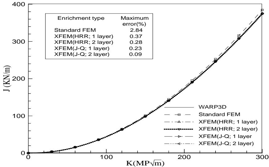Figure 9: Comparison of the $J$ -integral computed by using WARP3D with the one by using the XFEM for the biaxiality parameter $B$ of -0.5

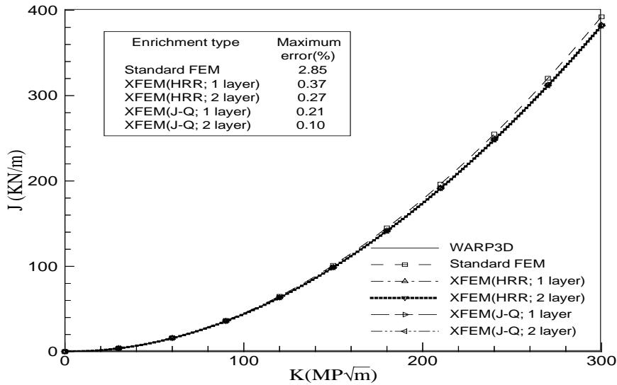Figure 10: Comparison of the $J$ -integral computed by using WARP3D with the one by using the XFEM for the biaxiality parameter $B$ of 0.0

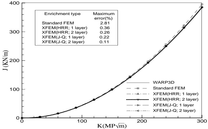Figure 11: Comparison of the $J$ -integral computed by using WARP3D with the one by using the XFEM for the biaxiality parameter $B$ of 1.0 As shown these figures, the $J - Q$ enrichment gives more accurate results for the $J$ -integral as compared with the HRR one. Moreover, even the $J - Q$ enrichment with 1-layer improves the numerical accuracy for the $J$ -integral than the HRR one with 2-layer.

Figure 12 depicts the distribution of the Von-Mises equivalent stress computed by the XFEM corresponding to the $J - Q$ enrichment with 2-layer for the $B = -0.5$ and $K_{I} = 300MPa\sqrt{m}$.

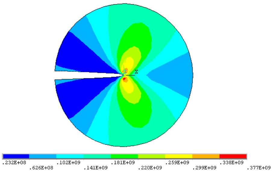Figure 12: Distribution of the Von-Mises equivalent stress computed by the XFEM corresponding to the $J - Q$ enrichment with 2-layer for the $B = -0.5$ and $K_{I} = 300MPa\sqrt{m}$

b) $SE(T)$ and $DE(T)$

The $J$ -integral can be composed as the sum of the elastic part and the plastic one as follows [23].

$$ J = J _ {e} + J _ {p} \tag {19} $$

Here, $J_{e}$ is the elastic part which is expressed as

$$ J _ {e} = f \frac {P ^ {2} \pi a}{E ^ {*}} \tag {20} $$

where, $f$ is the shape factor depending on the loading mode and the crack geometry, $P$ is the far-filed applied load, $a$ is a crack length and $E^{*}$ is the Young's modulus representing $E^{*} = E$ for the plane strain and $E^{*} = E / (1 - \nu^{2})$ for the plane strain. It should be noted that the plasticity-corrected $J_{e}$ has to be used due to the crack tip yielding.

In general, $J_{p}$ is expressed as

$$ J_{p} = \alpha \varepsilon_{0} \sigma_{0} g \lambda \left(\frac{P}{P_{0}}\right)^{n+1} $$

where, $g$ is a constant depending on the crack geometry, $\lambda$ a parameter related with the crack geometry and the strain hardening exponent and $P_0$ is the limit load.

All the analytical formula are taken as in ref [23, 27].

i. $SE(T)$ specimen

Figure 13 shows the geometry of SE(T) specimen.

The material characteristics is assumed as $n = 10$, $E / \sigma_0 = 500$, $E = 206GPa$ and $\nu = 0.3$. The plane strain is assumed with $W = 1m$ and $L = W$. The element size is taken as $W / 40$ for all the cases. The full model with the relative crack length of $a / W = 0.25$, 0.5 and 0.75 is used, respectively.

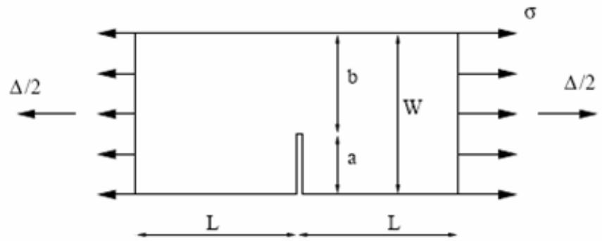Figure 13: Geometry of SE(T) specimen

Figure 14~figure 16 shows the comparison of the analytical $J$ -integral with the numerical one by the XFEM for the various crack length increasing the external load $\sigma$, respectively.

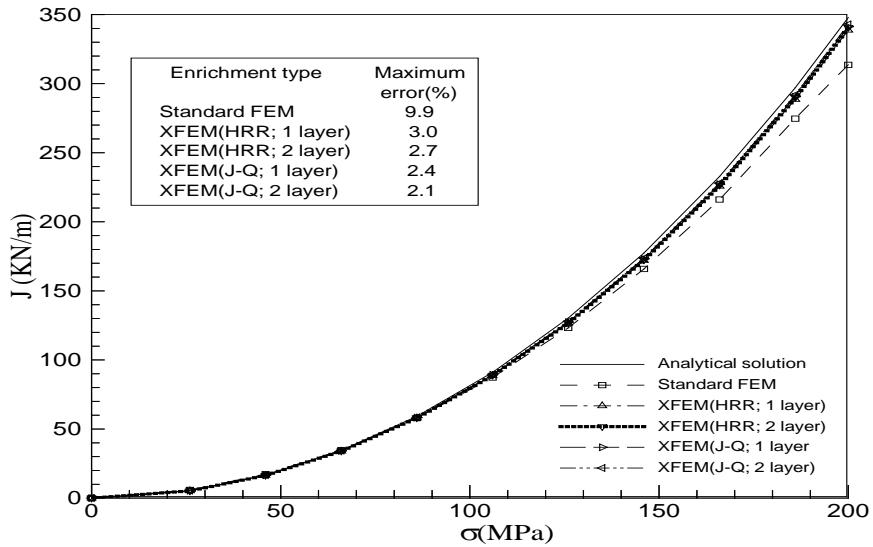Figure 14: Comparison of the analytical $J$ -integral with the numerical one by the XFEM for the SE(T) specimen with the relative crack length of $a / W = 0.25$

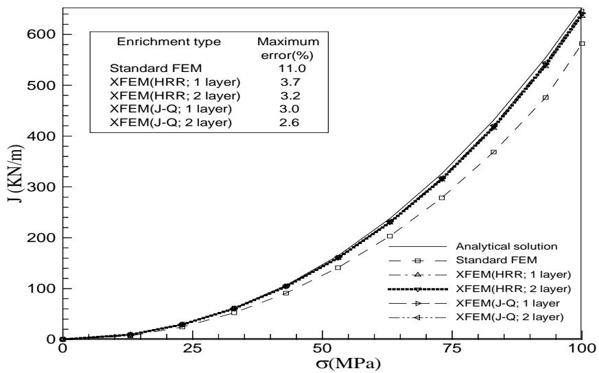Figure 15: Comparison of the analytical $J$ -integral with the numerical one by the XFEM for the SE(T) specimen with the relative crack length of $a / W = 0.5$

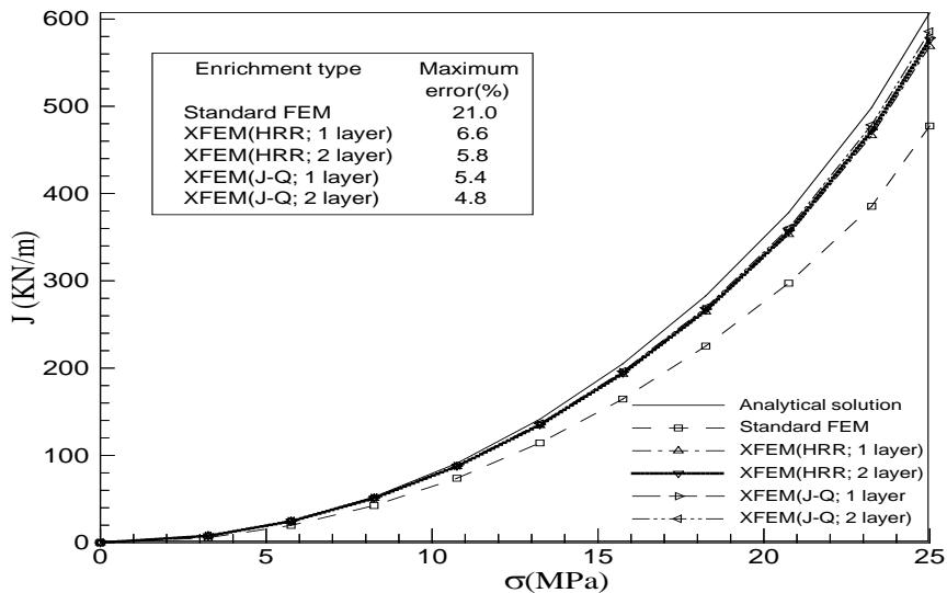Figure 16: Comparison of the analytical $J$ -integral with the numerical one by the XFEM for the SE(T) specimen with the relative crack length of $a / W = 0.75$

As shown these figures, the $J - Q$ enrichment gives more accurate results for the $J$ -integral as compared with the HRR one. The $J - Q$ enrichment improves the numerical accuracy of the $J$ -integral by about 0.6% for the SE(T) specimens with the relative crack length of $a / W = 0.25$ and 0.5 and by 1~1.2% for the one of $a / W = 0.75$ as compared with the HRR enrichment when employing the same enriched layers.

Moreover, even the $J - Q$ enrichment with 1-layer improves the numerical accuracy for the $J$ -integral than the HRR one with 2-layer.

ii. $DE(T)$ Specimen

Figure 17 shows the geometry of DE(T) specimen.

Two material properties are assumed as follows;

$$ n = 5, E / \sigma_ {0} = 8 0 0, E = 2 0 6 G P a \text{and} \nu = 0.3 $$ $$ n = 2 0, E / \sigma_ {0} = 3 0 0, E = 2 0 6 G P a \text{and} \nu = 0.3 $$

The plane strain is assumed with $W = 1m$, $L = 1.5W$ and $a / W = 0.5$. The element size is taken as $W / 40$ for all the cases. The half model is used due to the symmetry about the middle plane perpendicular to the crack line. The topological enrichment with 1-layer and 2-layer is employed for the region near the crack tip.

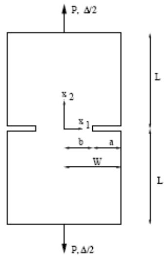Figure 17: Geometry of DE(T) specimen

Figure 18 and figure 19 compares the analytical solution with the numerical one done by the XFEM with different enrichments for the DE(T) specimen with the strain hardening exponent of $n = 5$ and $n = 20$, respectively.

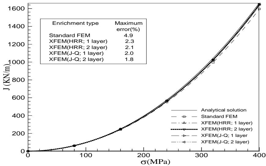Figure 18: Comparison of the analytical solution with the numerical one done by the XFEM with different enrichments for the DE(T) specimen with the strain hardening exponent of $n = 5$

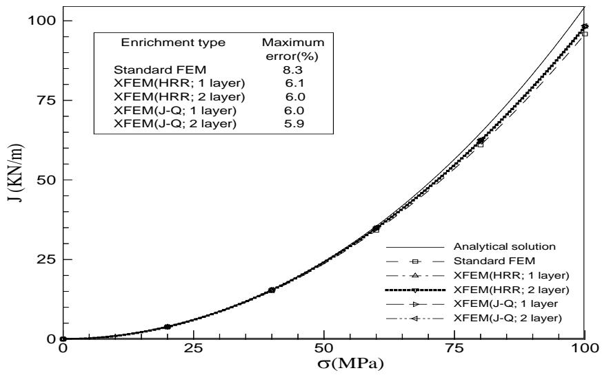Figure 19: Comparison of the analytical solution with the numerical one done by the XFEM with different enrichments for the DE(T) specimen with the strain hardening exponent of $n = 20$

As seen these figure, the $J - Q$ enrichment gives more accurate result for the $J$ -integral as compared with the HRR one like the SE(T) specimen.

Furthermore, even the $J - Q$ enrichment with 1-layer improves the numerical accuracy for the $J$ -integral than the HRR one with 2-layer.

VII. CONCLUSION

In this paper, we proposed a family of crack tip enrichment function for the XFEM implementation of elastic-plastic crack, based on the $J - Q$ theory. Such a family of crack tip enrichment function consists of 9 enrichment functions in total, namely, 6 ones previously proposed based on the HRR singular field as well as 3 ones taking account for the crack tip constraint effect. The FEA of the MBL model by using WARP3D was conducted in order to the higher terms for the crack tip displacement field, leading to the suggestion of 3 additional enrichment functions which gave the good estimation for the higher terms in the asymptotic expansion of elastic-plastic crack tip displacement field as well as the global crack tip displacement field. The introduction of these functions into the XFEM enrichment functions enables to improve the approximation of crack tip displacement field significantly.

In numerical analysis for the validation of proposed enrichment functions, crack faces were coincident with element boundaries and a crack tip is taken as a node, in order to eliminate other possible errors besides error concerned with the crack tip enrichment functions. By using the general purpose finite element software ANSYS, 2-dimensional elastic-plastic XFEM was implemented for the MBL model as well as various fracture specimens. Numerical result showed that the enrichment functions suggested by ours could improve the accuracy of fracture parameters significantly as compared with ones based on HRR field. Moreover, even the $J - Q$ enrichment with 1-layer improved the numerical accuracy for the $J$ -integral than the HRR one with 2-layer.