I. INTRODUCTION

It is a crucial problem in theory of communications if the average speed of information transfer over a noisy channel of finite bandwidth is bounded. That was a seminal result by Shannon (Shannon, 1948) 72 years ago. It is high time, however, to take this result under a magnifying glass, while all kinds of appreciations are given. The long-elapsed time since its discovery proves that the result is robust, it is not easy to find anything to refine.

This almost impossible task is the goal of our paper. Our motivation is to explain the deviation between the Shannon formula and our Matlab/Simulink experiment with a noise insensitive circuit (Ladvánszky, 2020).

II. PROBLEM STATEMENT

In this Section an experiment is described that cannot be characterized by the Shannon formula.

Let us start with the Shannon formula (Shannon, 1948).

where C is said to be channel capacity, W is the so-called channel bandwidth, S and N are signal and noise average power.

In our Matlab/Simulink experiment (Ladvánszky, 2020), a noisy 4QAM signal is recovered by a modified Costas loop. W = 4 MHz, $\frac{S}{N}=-13$ dB, and the 2 MS/s signal is recovered at SER < 0.001 (symbol error rate).

Substituting these data into (1), the result is $C\approx 282$ kS/s, and that roughly deviates from the speed of the recovered signal. As a conclusion, the Shannon formula is not valid for this case.

III. A Possible Solution: A New Formula

In this Section, we gather some facts in connection with the Shannon formula. After some criticism, a new formula is derived that can characterize the experimental fact mentioned in the previous Section.

We start with the classical model of communications, (Shannon, 1948), Figure 1:

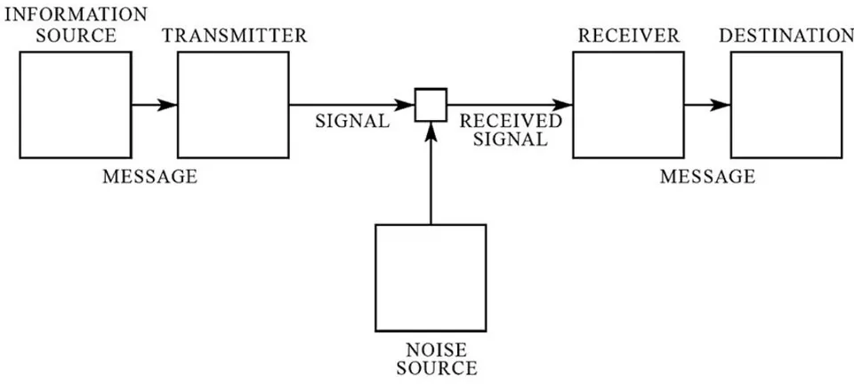
At the center of Figure 1, the small square is the channel. In this paper, we define the channel as a broad-band system block that represents propagation of electromagnetic waves from the transmitter to the receiver. Examples for channel in this sense is a piece of coaxial cable or optical fiber.

The channel in Figure 1 does not contain any filters. Filters are parts of the transmitter and the receiver.

We have three bandwidths in consideration. W is the channel bandwidth, we mean the bandwidth of the channel defined above. In case of coaxial cables, its value is some hundreds of MHz or in the GHz range.

$B_S$ is the signal bandwidth. It is determined by the transmitted signal in the baseband. Its meaning is clarified in Figure 2, its value is 4 MHz in our experiment.

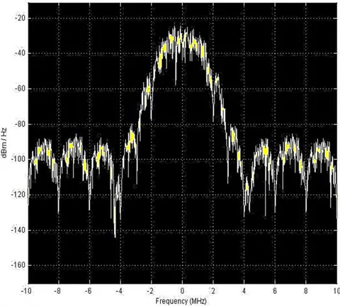
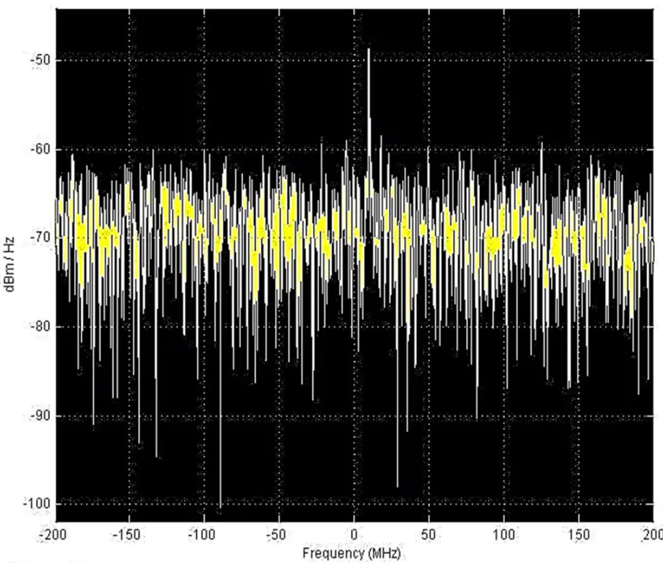
$B_S=4$ MHz, $B_N$ is the noise bandwidth, Figure 3. In our experiment, it is 200 MHz.

Equation (1) is valid for the case when signal and noise bandwidths are identical (Shannon, 1948).

Our first objection is that C is not a characteristic of the channel alone. For example, S is signal power, a characteristic of the transmitter and not the channel, and W is also questionable. We call here C as upper bound of average speed of information transfer, it is a characteristic of the whole communication system consisting of a transmitter, a channel, and a receiver.

Original explanation for $C$ is (Shannon, 1948), Theorem 12; (Shannon, 1949), (1).

where ${\log }_{2}M$ is the maximum number of correctly transferred bits. Averaging time is exceptionally long. Name of upper bound for average bitrate is correct.

In (Shannon, 1948), signal bandwidth $B_S$ and noise bandwidth $B_N$ are identical and it is called as channel bandwidth W:

where spectra are defined as follows:

where PDS and PDN are power densities, assumed frequency independent.

In the original papers (Shannon, 1948, 1949), the following assumption is hold:

However, in the model of Figure 1, in general,

Notes

As is not reasonable, $B_S\le B_N$. Signal to noise ratio is:

Combining (4, 5, 6, 8)

In general,

If (7) holds, then

We introduce a new quantity $C^{\prime }$ That is the formal extension of (1) for the case of non-identical bandwidths:

In order to extend (1) for the case of non-identical bandwidths (7), let us start from the Shannon formula for colored noise (Shannon, 1949), Equation (32):

By combining (4, 5, 12), we obtain

It is exploited that PDS and PDN do not depend on f. (13) is valid for the case of non-identical bandwidths (7), while (1) is not valid.

If , then , as we realized it in a Matlab/Simulink experiment with our version of the modified Costas loop (Ladvánszky, 2020).

So, . $C^{\prime }$ is the formal extension of the Shannon formula, $C_1$ is our formula. Can we say now if the Shannon formula is exceeded? Author's opinion is yes if also a physical circuit realization is produced. The circuit should operate with low symbol error rate at a SNR negative in dB. This experiment is coming soon.

IV. CONSEQUENCES: BOUNDS FOR THE AVERAGE SPEED OF COMMUNICATIONS Lower bound for operation of the circuit is:

From (12) and (14):

Notes

Average speed of information transfer is bounded from below by the signal bandwidth. That is natural and obvious. Considering (12) for fixed $B_S$ and PDS, we see that $C_1$ is bounded from above by the smallest possible PDN only. That is the cosmic background radiation (Bucher, 2015) or the thermal noise (Kerr & Randa, 2010), which is greater. At the moment, we can see another limiting factor.

Carrier frequency $f_c$. In order to be able to reconstruct the carrier,

This is because the lower edge of the lower sideband around $f_c$, should be at a positive frequency.

In our 4QAM experiment, actual transfer speed is 2 MS/s and the carrier frequency is 10 MHz.

Now we substitute (16) back into (13):

Meaning of (17) is that a $\frac{PDS}{PDN}$ value greater than that in (17), cannot be exploited for further increasing the bitrate. For control, we read the power density values from Figure 3. PDS = -52 dBm/Hz, PDN = -72 dBm/Hz, and we also know that $B_S=4MHz$, $f_c=10MHz$. Then in (17), $\frac{PDS}{PDN}=100$ and $2^{\frac{f_c}{BS}}-1\approx 4.66$ so in this case $f_c$ limits the maximum bitrate that can be achieved with increasing PDS.

We can calculate how much it is. Substituting these values in (13), $C_1\approx 26.6$ Mb/s, and due to the limitation by $f_c$, $C_1=10$ Mb/s could be achieved in ideal case.

We discussed some concepts in connection with the Shannon formula. We derived a modification of the original formula and concluded that speed of communications can be higher than that we believed.

If the reader checks the keyword "digital communications pdf" in an internet browser, then it gives more than 20 choices (Proakis & Salehi, 2015). Most of them consider W as channel bandwidth and make signal and noise bandwidths identical. So, our present discussion is timely.

Our derivation is valid if the channel signal is real. The relations are easy to extend for the case of complex signals, however.

It can be clearly recognized that the whole thing depends on the definition of bandwidths. Author's experience is that the typical misunderstanding is as follows. The channel bandwidth is limited to the signal bandwidth and thus a part of the noise spectrum is neglected in calculation of $SNR$. This error occurs if one considers the receiver filter as part of the channel.

We call the attention of the reader to a fine moment in derivation of (13). The same equation can also be achieved when we substitute equal bandwidths (6) in (1a). But what we do is different. We consider different bandwidths (7) and the result in (13) is the consequence of the fact that the upper limit of integration is lower than $B_N$ in (12).

We are aware, by comparison of Figure 2 and Equation (4), that Equation (4) is an approximation. However, considering the exact value of $S(f)$ is straightforward.

The author is also available on ResearchGate, LinkedIn and Facebook.

ACKNOWLEDGEMENTS

The author is grateful to Dr.

I. Schmideg who called his attention to check the Shannon formula. Dr. E. Simonyi is also acknowledged for the constant encouragement as the advisor of the DSc work of the author. The Hungarian team representing the medicine NORMALIFE is acknowledged for their significant improvement to the health of the author.