## I. GRAVITY Einstein approached the interaction between gravity and light by the introduction of the "Einstein Gravitational Constant" in the 4-dimensional Energy-Stress Tensor. $$ \mathrm{G}_{\mu \nu} + \Lambda \, g_{\mu \nu} = \kappa \, \mathrm{T}_{\mu \nu} $$ In which $\mathbf{G}_{\mu \nu}$ equals the Einstein Tensor, $\mathbf{g}_{\mu \nu}$ equals the Metric Tensor, $\mathrm{T}_{\mu \nu}$ equals the Stress-Energy tensor, $\Lambda$ equals the cosmological constant and $\pmb{K}$ equals the Einstein gravitational constant. An alternative approach to Einstein's expression with the tensor $\kappa \mathbf{T}_{\mu \nu}$, describing the curvature of the Space-Time continuum, is the sum of the Electromagnetic Tensor $\mathbf{T}_{\mu \nu}$ and the Gravitational Tensor $\mathbf{J}_{\mu \nu}$. $$ \kappa_{\mu \nu} \mathrm{T} \Leftrightarrow \underset{\mu \nu}{\mathrm{T}}_{\mu \nu} + \mathrm{J} \tag{2} $$ The 4-dimensional divergence of the sum of the Electromagnetic Stress-Energy tensor and the Gravitational Tensor expresses the 4-dimensional Force-Density vector (expressed in [N/m3] in the 3 spatial coordinates) as the result of Electro-Magnetic-Gravitational interaction. $$ f ^ {\mu} = \partial_ {v} \left(\mathrm {T} ^ {\mu v} + \mathrm {J} ^ {\mu v}\right) \tag {3} $$ In vector notation the 4-dimensional Force-Density vector can be written as: $$ \overline {{f}} ^ {4} = \left( \begin{array}{l} f _ {4} \\f _ {3} \\f _ {2} \\f _ {1} \end{array} \right) = \square \square \left(\overline {{\overline {{\mathbf {T}}}}} + \overline {{\overline {{\mathbf {J}}}}}\right) \tag {4} $$ The fundamental boundary condition for this alternative approach to gravity is the requirement that the Force 4 vector equals zero in the 4 dimensions, expressing a universal 4-dimensional equilibrium: $$ \overline {{f}} ^ {4} = \left( \begin{array}{l} f _ {4} \\f _ {3} \\f _ {2} \\f _ {1} \end{array} \right) = \square \square \left(\overline {{\overline {{\mathbf {T}}}}} + \overline {{\overline {{\mathbf {J}}}}}\right) = \overline {{0}} ^ {4} \tag {5} $$ The 3 spatial components of the Force-Density vector, as a result of Electro-Magnetic-Gravitational interaction can be written as: $$ \begin{array}{l} \overline{f} = \frac{1}{c^{2}} \frac{\partial (\overline{\mathrm{E}} \times \overline{\mathrm{H}})}{\partial t} + \varepsilon_{0} \overline{\mathrm{E}} (\nabla \cdot \overline{\mathrm{E}}) - \varepsilon_{0} \overline{\mathrm{E}} \times (\nabla \times \overline{\mathrm{E}}) + \\+ \mu_{0} \overline{\mathrm{H}} (\nabla \cdot \overline{\mathrm{H}}) - \mu_{0} \overline{\mathrm{H}} \times (\nabla \times \overline{\mathrm{H}}) + \gamma_{0} \overline{\mathbf{g}} (\nabla \cdot \overline{\mathbf{g}}) - \gamma_{0} \overline{\mathbf{g}} \times (\nabla \times \overline{\mathbf{g}}) = \overline{0} [\mathrm{N} / \mathrm{m}^{3}] \\end{array} $$ $$ \varepsilon_ {0} (\nabla . \bar{\mathrm{E}}) = \rho_ {\mathrm{E}} \text{ElectricChargeDensity} [ \mathrm{C} / \mathrm{m} ^ {3} ] $$ in which: $\mu_0(\nabla.\overline{\mathrm{H}}) = \rho_M$ Magnetic Flux Density [Vs/ m3] or [Wb/ m3](6) $$ \gamma_0 (\nabla \cdot \bar{\mathrm{g}}) = \rho_M \text{Mass Density (Electromagnetic)} [\mathrm{kg}/\mathrm{m}^3] $$ $$ \text {E l e c t r i c E n e r g y D e n s i t y :} \quad \mathrm {w} _ {\mathrm {E}} = \frac {1}{2} \varepsilon_ {0} \mathrm {E} ^ {2} $$ $$ Magnetic Energy Density: \quad w_{\mathrm{M}} = \frac{1}{2} \mu_0 \hat{\mathrm{H}} $$ $$ Gravitational Energy Density: \mathrm{w}_\mathrm{G} = \frac{1}{2} \gamma_0 \mathrm{g}^2 $$ In which $E$ represents the electric field intensity expressed in $[V/m]$, $H$ represents the magnetic field intensity expressed in $[A/m]$ and $g$ represents the gravitational acceleration expressed in $[m/s^2]$. The permittivity indicated as $\varepsilon_0$, the permeability indicated as $\mu_0$ and the gravitational permeability of vacuum as $\gamma_0$. For curl-free gravitational fields equation (6) can be written as: $$ \overline{f} = \frac{1}{c^{2}} \frac{\partial (\overline{\mathrm{E}} \times \overline{\mathrm{H}})}{\partial t} + \varepsilon_{0} \overline{\mathrm{E}} (\nabla \cdot \overline{\mathrm{E}}) - \varepsilon_{0} \overline{\mathrm{E}} \times (\nabla \times \overline{\mathrm{E}}) + \\+ \mu_{0} \overline{\mathrm{H}} (\nabla \cdot \overline{\mathrm{H}}) - \mu_{0} \overline{\mathrm{H}} \times (\nabla \times \overline{\mathrm{H}}) + \overline{\rho}_{M} = \overline{0} \[\mathrm{N}/\mathrm{m}^{3}] $$ Substituting Einstein's $W = m c2$ in (7) results in "Electro-Magnetic-Gravitational Equilibrium Field Equation" (8): $$ \begin{array}{l} \overline{f} = \frac{1}{c^{2}} \frac{\partial (\overline{\mathrm{E}} \times \overline{\mathrm{H}})}{\partial t} + \varepsilon_{0} \overline{\mathrm{E}} (\nabla \cdot \overline{\mathrm{E}}) - \varepsilon_{0} \overline{\mathrm{E}} \times (\nabla \times \overline{\mathrm{E}}) + \\+ \mu_{0} \overline{\mathrm{H}} (\nabla \cdot \overline{\mathrm{H}}) - \mu_{0} \overline{\mathrm{H}} \times (\nabla \times \overline{\mathrm{H}}) + \frac{1}{2 c^{2}} \overline{\mathrm{g}} (\varepsilon \mathrm{E}^{2} + \mu \mathrm{H}^{2}) = \overline{0} \[\mathrm{N}/\mathrm{m}^{3}] \tag{8} \\end{array} $$ The theory presented outlines the interactions between electromagnetic-gravitational, magnetic-gravitational, and electric-gravitational fields. A key distinction in this new theory is that particles do not directly interact with fields; rather, interactions occur between the fields themselves. For instance, when an electrically charged particle interacts with an electric field, this interaction is not particle-to-field but rather an interplay between the electric fields associated with each entity. This concept extends to all interactions within the theory: Electric fields interact with electric fields, magnetic fields interact with magnetic fields, and gravitational fields interact with gravitational fields. Therefore, every interaction is essentially a dynamic exchange between these respective fields rather than direct particle-field interactions. This framework emphasizes the critical role of field interactions in shaping the behavior and dynamics of particles and offers a unique perspective on the fundamental forces at play in the universe. ## II. "GRAVITATIONAL REDSHIFT/BLUESHIFT IN LIGHT (EMR)" DUE TO ### "ELECTROMAGNETIC GRAVITATIONAL INTERACTION" In order to evaluate the New Theory, the experiment on Gravitational Redshift, titled "Test of the Gravitational Redshift with Galileo Satellites in an Eccentric Orbit" authored by S. Hermann and colleagues, has been selected. For this particular experiment, a stable frequency from a ground station's MASER was transmitted to 2 Galileo Satellites, with the goal of analyzing the frequency variance between the ground station and the satellites. The gravitational field of the Earth induced the frequency shift, and 2 satellites were specifically chosen to offset the eccentricity of the Galileo Orbit. If we consider a gravitational field $g[z]$ that varies along the radial axis in Cartesian coordinates connecting the ground station to the satellites: $$ \overline{{\mathrm{g} [ \mathrm{z} ]}} = \left\{0, 0, \frac{\mathrm{G M} _ {\text{Earth}}}{4 \pi \mathrm{z} ^ {2}} \right\} \tag{9} $$ In which $G(G = 6.67428 \, 10^{-11} \, \text{Nm}^2 / \text{kg}^2)$ equals the Gravitational constant, $M_{\text{Earth}}$ the mass of the earth and $r$ the radial distance from the centre of the earth. The mathematical solution [5] of equation (8) for plane electromagnetic waves (expressed in cartesian $\{x,y,z\}$ coordinates) related to the Electric Field Intensity equals: $$ \bar{\mathrm{E}} = \left( \begin{array}{l} \mathrm{E} _ {\mathrm{x}} \\\mathrm{E} _ {\mathrm{y}} \\\mathrm{E} _ {\mathrm{z}} \end{array} \right) = \left( \begin{array}{c} \mathrm{e} ^ {- \frac{\mathrm{G M} _ {\text{Earth}} \varepsilon_ {0} \mu_ {0}}{8 \pi z}} \mathrm{h} \left[ \omega_ {0} \mathrm{e} ^ {- \frac{\mathrm{G M} _ {\text{Earth}} \varepsilon_ {0} \mu_ {0}}{4 \pi z}} (\mathrm{t} - \sqrt{\varepsilon \mu} z) \right] \\0 \\0 \end{array} \right) \tag{10} $$ And the mathematical solution of (8) for the Magnetic Field Intensity equals: $$ \overline{{\mathrm{H}}} = \binom{\mathrm{H} _ {\mathrm{x}}} {\mathrm{H} _ {\mathrm{y}}} = \left( \begin{array}{c} 0 \\\frac{1}{\sqrt{\varepsilon_ {0} \mu_ {0}}} \mathrm{e} ^ {- \frac{\mathrm{G M} _ {\text{Earth}} \varepsilon_ {0} \mu_ {0}}{8 \pi z}} \mathrm{h} \left[ \omega_ {0} \mathrm{e} ^ {- \frac{\mathrm{G M} _ {\text{Earth}} \varepsilon_ {0} \mu_ {0}}{4 \pi z}} (\mathrm{t} - \sqrt{\varepsilon \mu} z) \right] \\0 \end{array} \right) \tag{11} $$ In this scenario, the original frequency of the MASER radiation traveling in the direction of the Earth's gravitational field $g[z]$ is represented by $\omega_0$. The presence of the exponential term signifies the Gravitational Redshift experienced when the MASER radiation moves in the Earth's Gravitational Field. Although the speed of propagation of Electromagnetic Radiation (the speed of light) remains constant, both the field intensity's amplitude and frequency experience an exponential decrease. Mathematica calculations compare the results obtained from General Relativity with those from the New Theory. By setting the distance from the ground station to the Earth's center as $z_{1} = 6,378,000$ [m](Earth's radius) and the average distance of ESA satellites in a Galileo orbit as $z_{2} = 23,222,000$ [m](distance from the ESA satellite to the Earth's center), the Gravitational Redshift according to General Relativity is determined to be: $$ \Delta \omega_{GR} = 0.00000000004011815497097883 \, [\mathrm{s}^{-1}] \tag{12} $$ Calculated with Mathematica, the Gravitational RedShift according to the New Theory, which is a solution of equation (8) equals: $$ \Delta \omega_ {G R} = 0. 0 0 0 0 0 0 0 0 0 4 0 1 1 8 2 4 2 0 6 1 7 3 7 4 2 [ \mathrm {s} ^ {- 1} ] \tag {13} $$ Both calculated values a within the Range of the measured gravitational RedShift by the average values of both ESA satellites in the Galileo orbit $$ \Delta \omega_ {\text{Measured}} = 0.0 0 0 0 0 0 0 0 0 0 4 0 1 1 8 \quad \pm 2.2 1 0 ^ {- 1 5} \quad [ \mathrm{s} ^ {- 1} ] \tag{14} $$ In [2] a factor has been defined which presents the measured deviation between the predicted Gravitational RedShift by General Relativity and the Measured Gravitational RedShift. $$ \alpha = \Delta \omega_ {\text{MEASURED}} - \Delta \omega_ {\mathrm{G R}} = (2.2 \pm 1.6) \times 1 0 ^ {- 5} \tag{15} $$ A comparable factor can be used to determine which theory (General Relativity or the New Theory) has the nearest approach to the experimentally measured data. Highly accurate measuring experiments are required with an accuracy higher than 16 digits beyond the decimal point. ## III. BLACK HOLES ### a) Black Holes without Singularities with dimensions smaller than the diameter of the Hydrogen Atom A second fundamental solution for equation (8) describes a Gravitational Electromagnetic Confinement (BLACK HOLE) [1] within a radial gravitational field with acceleration (in radial direction). This solution represents a Black Hole, the confinement of light due to its own gravitational field, and has no singularities. This solution for equation (8) describes Black Holes, dependent of time and radius, presenting discrete spherical energy levels, within a radial gravitational field with acceleration (in radial direction)[14]has been represented in (16) and (17). $$ \left( \begin{array}{l} E _ {r} \\E _ {\theta} \\E _ {\varphi} \end{array} \right) = \left( \begin{array}{c} 0 \\\mathrm {f (r)} \quad \mathrm {S i n (k r)} \quad \mathrm {S i n (\omega t)} \\- \mathrm {f (r)} \quad \mathrm {C o s (k r)} \quad \mathrm {C o s (\omega t)} \end{array} \right) \quad \left( \begin{array}{l} H _ {r} \\H _ {\theta} \\H _ {\varphi} \end{array} \right) = \sqrt {\frac {\varepsilon}{\mu}} \left( \begin{array}{c} 0 \\- \mathrm {f (r)} \quad \mathrm {S i n (k r)} \quad \mathrm {C o s (\omega t)} \\- \mathrm {f (r)} \quad \mathrm {C o s (k r)} \quad \mathrm {S i n (\omega t)} \end{array} \right) \quad \overline {{g}} = \left( \begin{array}{c} G _ {1} \\\frac {4 \pi r ^ {2}}{} \\0 \\0 \end{array} \right) $$ $$ \mathrm {w} _ {\mathrm {e m}} = \left(\frac {\mu_ {0}}{2} \left(\bar {\mathrm {m}} . \bar {\mathrm {m}}\right) + \frac {\varepsilon_ {0}}{2} \left(\bar {\mathrm {e}} . \bar {\mathrm {e}}\right)\right) = $$ $$ f(r)^{2} \left(\left(\sin(\mathrm{kr}) \sin(\omega t)\right)^{2} + \left(\cos(\mathrm{kr}) \cos(\omega t)\right)^{2} + \frac{\varepsilon}{\mu} \left(\sin(\mathrm{kr}) \cos(\omega t)\right)^{2} + \left(\cos(\mathrm{kr}) \sin(\omega t)\right)^{2}\right) $$ In which the radial function $f(r)$ equals: $$ f [ r ] = K \mathrm{e} ^ { - \frac{ G M _ { \mathrm{ B H } } \varepsilon _ { 0 } \mu } { 8 \pi r } } $$ Grepresents the Gravitational constant and Mrepresents the total confined electromagnetic mass of the BLACK HOLE. Equation (16) presents a Standing (Confined) Electromagnetic Field Configuration with a phase shift of 90 degrees between the electric field and the magnetic field with the corresponding Nodes and Anti Nodes. [13]. The solution has been calculated according Newton's Shell Theorem. Assuming a constant speed of light "c" and Planck's constant $\hbar$ within the BLACK HOLE, the radius "R" (with $n = 1,2,3,4\ldots$ ) of the BLACK HOLE with the energy of a proton, according $W = m_{\text{proton}} c^2$, would be: $1.5009211 \times 10^{-10}[\mathrm{J}]$. $$ R _ {G E O N} = n \lambda = n \left(\frac {c}{f}\right) = n \left(\frac {c}{W}\right) \hbar = 7. 1 8 6 5 1 0 ^ {- 2 6} \left(\frac {n}{W}\right) $$ $$ \mathrm{R} _ {\text{GEON}} = \mathrm{n} 3.8 2 1 0 ^ {- 1 2} [ \mathrm{m} ] \tag{18} $$ Black Holes are varying from atomic dimensions with dimensions of 10-27 [kg], Page 39 [33] until Black Holes with dimensions of 1040 [kg], Page 67 [34]. At these dimensions Black Holes turn into Dark Matter. The fundamental boundary condition for the confinement of Electromagnetic radiation (BLACK HOLEs) is that the energy flow (Poynting vector) equals zero at the surface of the confinement. This is possible at every "90 degrees Phase Shift Surface" (Sphere) between the Electric Field and the Magnetic Field. ### b) Black Holes with a Singular point and Large dimensions Fig 1 represents a Black Hole with a mass of 1035 [kg] and a radius of about 25 [km] controlled by a different mahgematical solution for equation (8). The radius of the Black Hole equals about 25 [km] which has been controlled by a different mathematical solution (19) for equation (8). $$ f [ r ] = K \mathrm {e} ^ {\left(\frac {\mathrm {G M} _ {\mathrm {B H}} \varepsilon_ {0} \hbar}{8 \pi \mathrm {r}} - \log [ \mathrm {r} ]\right)} \quad [ \mathrm {J} / \mathrm {m} ^ {3} ] ^ {(1 9)} $$ 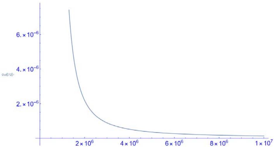 Fig. 1: The Energy Density [J/m3] as a function of the Radius $R = \max 107[m]$ of the Black Hole 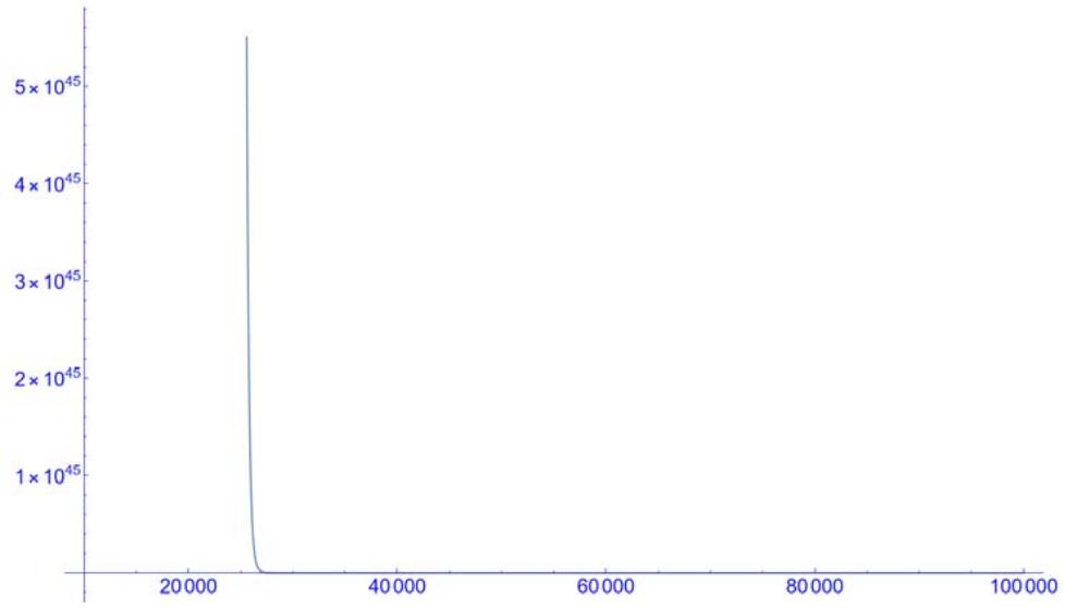 Fig. 2: The Energy Density [J/ m3] as a function of the Radius R = max 105 [m] Figures 1 and 2 showcase the significant impact of "Gravitational Intensity Shift" and "Gravitational RedShift" at a distance of $25\mathrm{km}$. Over a distance of $10,000\mathrm{km}$, the intensity of light emitted by a Black Hole with a mass of $10^{35}\mathrm{kg}$ decreases by a factor of $10^{-51}$. Similarly, the frequency of the emitted light from the Black Hole decreases by a factor of $10^{-51}$. For instance, light emitted in the visible spectrum at $10^{14}\mathrm{Hz}$ drops to a frequency of $10^{-37}\mathrm{Hz}$. These extremely low frequencies with minimal intensities have not been observed, leading to the term "Black Hole" being used to describe the phenomena of "Gravitational Intensity Shift" and "Gravitational RedShift" in the presence of a massive object. According to equation (8) and solutions (10) and (11), it is deduced that the speed of light remains constant within and around a Black Hole. The only potential change is in the direction of light propagation due to the influence of a gravitational field. ### c) Dark Matter in the Universe controlled by "Gravitational Shielding" Fig 3 represents Dark Matter with a total mass of $10^{53}$ [kg] and a radius of about 10 times the size of the Milky Way Galaxy. The radius of the dark mass equals 5 $10^{21}$ [m] which has been controlled by a different mathematical solution (20) for equation (8). 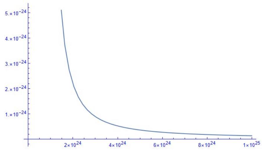$$ f[r]=K\mathrm{e}^{\left(\frac{G M_{\mathrm{BH}} \varepsilon_{0} \phi^\prime}{8 \pi r} - \log[r]\right)}\quad\left[\mathrm{J}/\mathrm{m}^{3}\right]^{(20)} $$  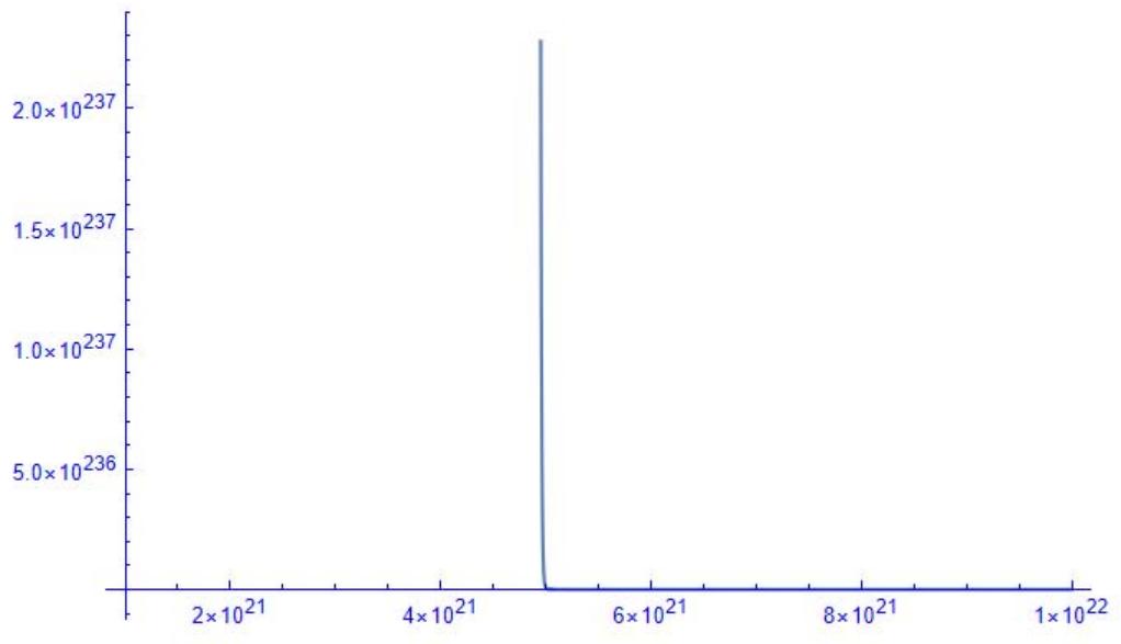 Fig. 3: The Energy Density $[\mathrm{J} / \mathrm{m}^3]$ as a function of the Radius $R = \max 10^{25}[\mathrm{m}]$ of the Dark Matter Figures 3 and 4 highlight the considerable impact of "Gravitational Intensity Shift" and "Gravitational RedShift" at a distance of $5 \times 10^{\wedge}21$ meters, which is equivalent to 10 times the radius of the Milky Way Galaxy. Over this vast distance, the intensity of the light emitted by Dark Matter with a mass of $10^{\wedge}53$ kg decreases by a factor of $10^{\wedge}$ -261. Similarly, the frequency of the emitted light from Dark Matter decreases by a factor of $10^{\wedge}$ -261. For example, light initially emitted in the visible spectrum at $10^{\wedge}14$ Hz drops to an incredibly low frequency of $10^{\wedge}$ -247 Hz. These incredibly low frequencies with extremely weak intensities have not been observed, leading to the term "Dark Matter" being assigned to describe the phenomena of "Gravitational Intensity Shift" and "Gravitational RedShift" in the presence of an immensely massive object. From equation (8) and the solutions (10) and (11), it is concluded that the speed of light remains constant within and around the Dark Matter. The only possible alteration is in the direction of light propagation due to the gravitational influence of the Dark Matter. ## IV. THE RELATIONSHIP BETWEEN BLACK HOLES AND QUANTUM PHYSICS Introducing the Quantum Vector Function $\overline{\phi}$, $$ \bar {\phi} = \sqrt {\frac {\mu}{2}} \left(\bar {H} + i \frac {\bar {E}}{c}\right) \tag {21} $$ Substituting (21) in (16) results in the quantum presentation for the BLACK HOLE: $$ \begin{array}{l} \overline{\Phi (r , \theta , \varphi)} = \sqrt{\frac{\mu}{2}} \left(\overline{\mathrm{H}} + \mathrm{i} \frac{\mathrm{E}}{c}\right) \mathrm{f} (\mathbf{r}) \left( \begin{array}{l} \Phi_{r} \\ \Phi_{\theta} \\ \Phi_{\varphi} \end{array} \right) \\ \overline{\Phi (r , \theta , \varphi)} = \alpha K t \sqrt{\frac{\varepsilon}{\mu}} e^{- \frac{G 1 \varepsilon_{0} \theta \mu}{8 \pi r}} \left( \begin{array}{ccc} 0 & 0 & 0 \\ 0 & - \sin (\mathrm{k} r) & \sin (\mathrm{k} r) \\ 0 & - i \cos (\mathrm{k} r) & i \cos (\mathrm{k} r) \end{array} \right) \left\{ \begin{array}{l} 0 \\ \operatorname{Cos} (\quad) \\ i \operatorname{Sin} (\quad) \end{array} \right\} \tag{22} \end{array} $$ With "K" a constant value dependend of the mass of the BLACK HOLE. The Dot product between the unit vector and the Quantum Vector Function $\bar{\phi}$ represents the quantum mechanical probability function $\Psi [r,t]$ which is a fundamental solution of the Schrödinger Wave Equation. $$ \begin{array}{l} \overline{{\Phi (r , \theta , \varphi)}} = K \omega t \sqrt{\frac{\varepsilon}{\mu}} e ^ {- \frac{G 1 \varepsilon_{0} \phi^{\prime}}{8 \pi r}} \left( \begin{array}{ccc} 0 & 0 & 0 \\ 0 & - \operatorname{Sin} (\mathrm{k r}) & \operatorname{Sin} (\mathrm{k r}) \\ 0 & - \mathrm{i} \operatorname{Cos} (\mathrm{k r}) & \omega \mathrm{t i} \operatorname{Cos} (\mathrm{k r}) \end{array} \right) \left\{ \begin{array}{ccc} 0 & & \\ \operatorname{Cos} (\quad) & & \\ \mathrm{i} \operatorname{Sin} (\quad) & & \end{array} \right\} \\ \Psi (\mathrm{r}, \mathrm{t}) = \left\{ \begin{array}{l} 1 \\ \omega \mathrm{t} \end{array} \right\} K e \sqrt{\frac{\varepsilon}{\mu}} = \frac{- G 1 \varepsilon_{0} \phi^{\prime}}{8 \pi \mathrm{r}} K e \sqrt{\frac{\varepsilon}{\mu}} - \frac{G 1 \varepsilon_{0} \phi^{\prime}}{8 \pi \mathrm{r}} e ^ {i \omega t} \tag{23} \end{array} $$ The Scalar function represents a fundamental solution of the Quantum Mechanical Schrödinger wave equation. 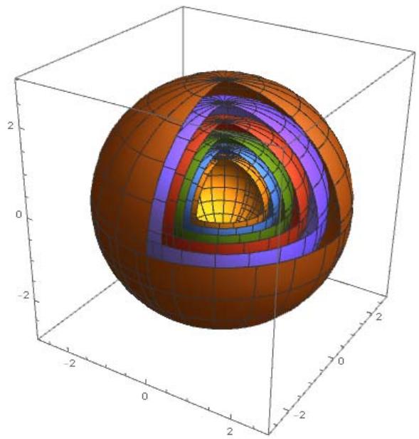[36, 37] ### a) Black Holes with Discrete Spherical Energy Levels at Sub-Atomic dimensions A critical condition for the containment of Electromagnetic Energy is that the Poynting vector equals zero at the spherical surface of the confinement. In the case of confinement within a sphere, a standing electromagnetic wave pattern necessitates the presence of concentric spheres. At each sphere, there exists an antinodal plane for either the electric field (E) or the magnetic field (B), with a distance in radius between each sphere equivalent to half the wavelength of the confinement. The constant $k$ is defined as $k = n^{*}\pi^{*}\lambda$, where "n" is a natural number (1, 2, 3, 4,...) and $\lambda$ represents the wavelength. i. Time and Radius dependent Black Holes with discrete Energy Levels. The confinements of Electromagnetic Radiation within spherical Regions Every concentric sphere represents an antinodal surface for the Electric Field (E) or the Magnetic Field (H). The Poynting Vector $\hat{\mathbf{S}} = \overline{\mathbf{E}}\times \overline{\mathbf{H}}$ at this spherical surface equals zero at any time and at any location at this sphere. The Electromagnetic Energy persists within each sphere and the subsequent concentric sphere. These concentric spheres are characterized by a difference in radius equivalent to half a wavelength of the electromagnetic radiation contained within the confinement, corresponding to distinct discrete energy levels. Each concentric sphere serves as an antinodal surface for either the electric field or the magnetic field.  Fig. 5: Nodal and Antinodal Spheres for Standing (Confined) Spherical Electromagnetic waves with a 90 degrees phase shift between the Electric field and the Magnetic field. Equation (9) 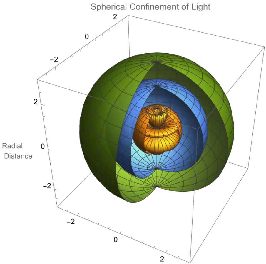 Fig. 6: Nodal- and Antinodal Spheres $(k = 3)$ for Standing (Confined) Spherical Electromagnetic waves with a 90 degrees phase shift between the Electric field and the Magnetic field. Equation (9) Equation (24) describes a Time and Radius dependent BLACK HOLE. $$ \overline{{\mathrm{E}}} = \mathrm{K e} ^ {- \frac{G 1 \varepsilon 0 \mu 0}{8 \pi r}} \left( \begin{array}{c} 0 \\\operatorname{Sin} [ \mathrm{k r} ] \operatorname{Sin} [ \omega t ] \\- \operatorname{Cos} [ \mathrm{k r} ] \operatorname{Cos} [ \omega t ] \end{array} \right) $$ $$ \overline{\mathrm{H}} = \mathrm{K} \, \mathrm{e}^{-\frac{G1\dot{0}0\mu0}{8\pi r}} \sqrt{\frac{\varepsilon_0}{\mu_0}} \left( \begin{array}{c} 0 \\\sin [ k r ] \cos [ \omega t ] \\- \cos [ k r ] \sin [ \omega t ] \end{array} \right) \tag{24} $$ Equation (20) represents by the function $\mathrm{Sin}[\mathrm{k}\mathrm{r}]$ ( $k = 1,2,3,4\ldots$ ) the confinement of electromagnetic radiation between two concentric spheres. K represents the amplitude of the Electric/ Magnetic Field Intensity. [14] ## ii. Time and Polar Angle dependent Black Holes 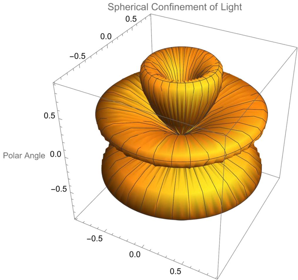 Fig. 7: Nodal- and Antinodal Polar Angle Regions (m = 3) for Standing (Confined) Spherical Electromagnetic waves with a 90 degrees phase shift between the Electric field and the Magnetic field. Equation (15) Equation (25) describes a Time and "Polar Angle" dependent BLACK HOLE $$ \overline{{\mathrm{E}}} = \mathrm{K e} ^ {- \frac{G 1 \varepsilon 0 \mu 0}{8 \pi r}} \left( \begin{array}{c} 0 \\\operatorname{Sin} [ \mathrm{m} \theta ] \operatorname{Sin} [ \omega \mathrm{t} ] \\\operatorname{Sin} [ \mathrm{m} \theta ] \operatorname{Cos} [ \omega \mathrm{t} ] \end{array} \right) $$ $$ \overline{\mathrm{H}} = \mathrm{K} \, \mathrm{e}^{-\frac{G1\delta0\mu0}{8\pi r}} \sqrt{\frac{\varepsilon_0}{\mu_0}} \left( \begin{array}{c} 0 \\\sin[\mathrm{m} \theta] \cos[\omega \mathrm{t}] \\- \sin[\mathrm{m} \theta] \sin[\omega \mathrm{t}] \end{array} \right) $$ Equation (19) represents by the function $\mathrm{Sin[m\theta](m = 1,2,3,4\dots)}$ the confinement of electromagnetic radiation between two Polar Angular Regions [15].  Fig. 4: The Energy Density $[\mathrm{J} / \mathrm{m}^3]$ of the Dark Matter as a function of the Radius $R = \max 10^{22}$ [m] 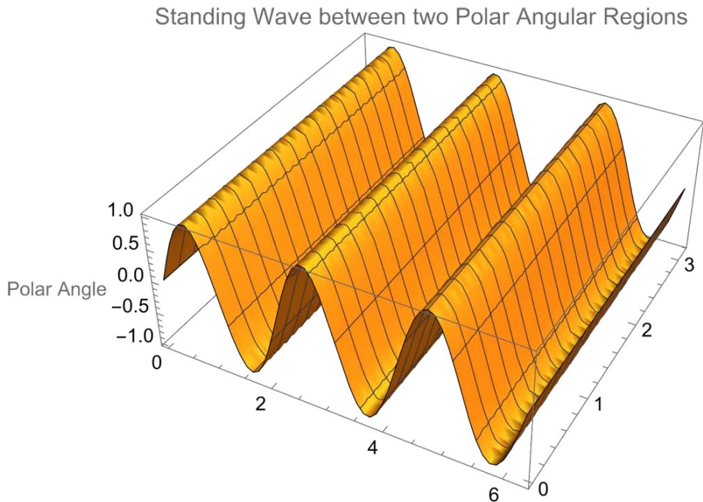 Fig. 8: Nodal- and Antinodal Polar Angle Regions (m = 3) for Standing (Confined) Electromagnetic waves with a 90 degrees phase shift between the Electric field and the Magnetic field. Equation (15) ## iii. Time and Azimuthal Angular dependent Black Holes 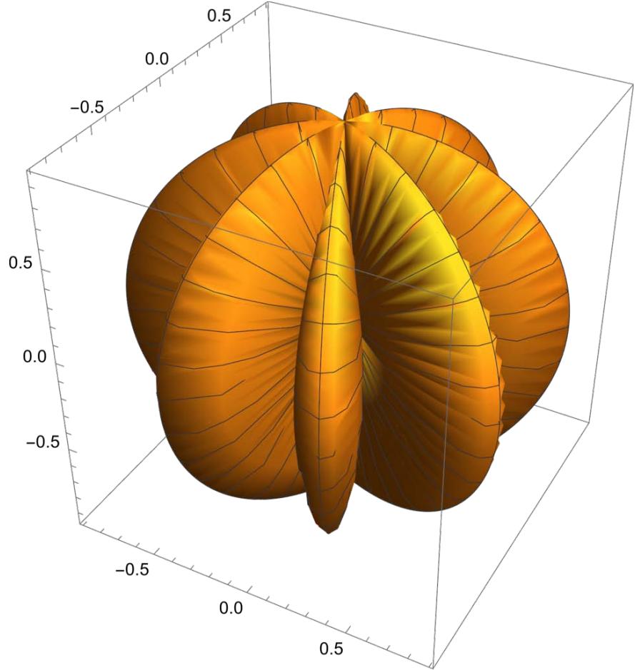 Fig. 9: Nodal- and Antinodal Azimuthal Angular Regions (n=3) for Standing (Confined) Electromagnetic waves with a 90 degrees phase shift between the Electric field and the Magnetic field. Equation (16) Equation (26) describes a Time and "Polar Angle" dependent BLACK HOLE $$ \overline{{\mathrm{E}}} = \textbf{K e} ^ {- \frac{G 1 \varepsilon 0 \mu 0}{8 \pi r}} \left( \begin{array}{c} 0 \\\operatorname{Cos} [ n \varphi ] \operatorname{Sin} [ \omega t ] \\\operatorname{Cos} [ n \varphi ] \operatorname{Cos} [ \omega t ] \end{array} \right) $$ $$ \bar{H} = K e ^ {- \frac{G 1 \dot{0} 0 \mu 0}{8 \pi r}} \sqrt{\frac{\varepsilon_ {0}}{\mu_ {0}}} \left( \begin{array}{c} 0 \\\operatorname{Cos} [ n \varphi ] \operatorname{Cos} [ \omega t ] \\- \operatorname{Cos} [ n \varphi ] \operatorname{Sin} [ \omega t ] \end{array} \right) \tag{26} $$ Equation (26) represents by the function $\mathrm{Sin}[\mathrm{n}\varphi ](\mathrm{n} = 1,2,3,4\dots \dots)$ the confinement of electro-magnetic radiation between two Azimuthal Angular Regions [16]. iv. Time, Polar- and Azimuthal Angular dependent Black Holes 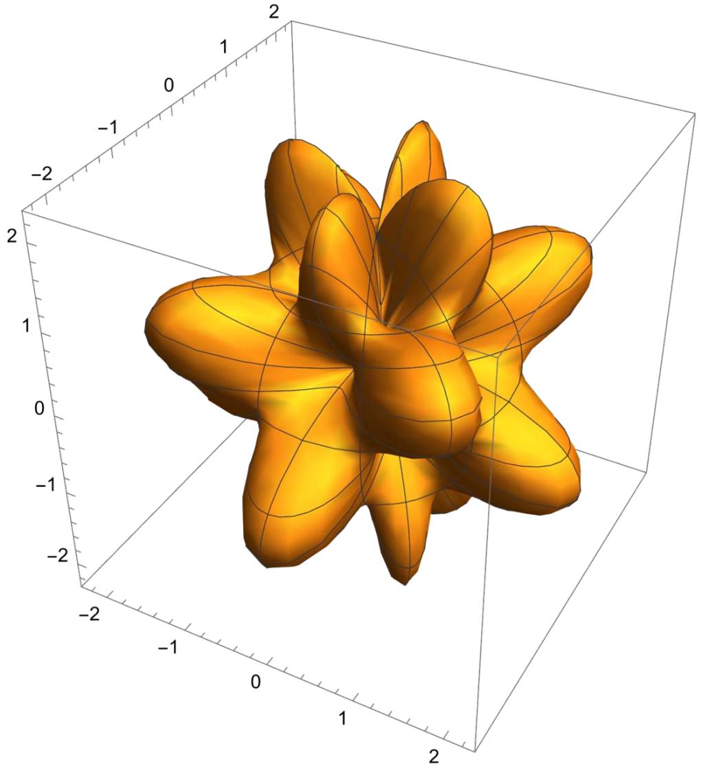 Fig. 10: Nodal- and Antinodal Polar Angular and Azimuthal Angular Regions (n = 4 and m = 4) for Standing (Confined) Electromagnetic waves with a 90 degrees phase shift between the Electric field and the Magnetic field. Equation (17) Equation (27) describes a Time "Azimuthal Angle" and "Polar Angle" dependent BLACK HOLE $$ \overline{{\mathrm{E}}} = \mathrm{K e} ^ {- \frac{G 1 \varepsilon 0 \mu 0}{8 \pi r}} \left( \begin{array}{c} 0 \\\operatorname{Cos} [ n \varphi ] \operatorname{Sin} [ m \theta ] \operatorname{Sin} [ \omega t ] \\\operatorname{Cos} [ n \varphi ] \operatorname{Sin} [ m \theta ] \operatorname{Cos} [ \omega t ] \end{array} \right) $$ $$ \bar{\mathrm{H}} = \mathrm{K e} ^ {- \frac{G 1 \dot{0} 0 \mu 0}{8 \pi r}} \sqrt{\frac{\varepsilon_ {0}}{\mu_ {0}}} \left( \begin{array}{c} 0 \\- \operatorname{Cos} [ n \varphi ] \operatorname{Sin} [ m \theta ] \operatorname{Cos} [ \omega t ] \\\operatorname{Cos} [ n \varphi ] \operatorname{Sin} [ m \theta ] \operatorname{Sin} [ \omega t ] \end{array} \right) \tag{27} $$ Equation (27) represents by the function $(n = 1,2,3,4\ldots)$ and $(m = 1,2,3,4\ldots)$ the confinement of electromagnetic radiation between two Azimuthal Angular Regions and two Polar Angular Regions [17]. v. Spherical Confinement of Light between two Concentric Spheres within Black Holess 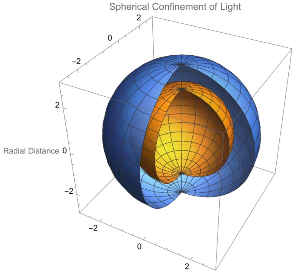 Fig. 11: Nodal- and Antinodal Regions for Standing (Confined) Electromagnetic waves with a 90 degrees phase shift between the Electric field and the Magnetic field. Equation (14) Equation (18) in the context of this theory illustrates the phenomenon of reflected electromagnetic energy confined within a Black Hole between two concentric spheres. Within this framework, the speed of light, influenced by the variable "r," undergoes directional changes in accordance with the frequency of the confined light, or electromagnetic radiation. A noteworthy concept introduced is the idea that a Black Hole has the potential to undergo a process of splitting into two distinct Black Holes with varying radii. During this process, the original Black Hole transitions to a lower energy state while the newly formed Black Hole embodies the energy differential, akin to an atom transitioning to a lower energy level. This analogy underscores the dynamic nature of Black Holes and the intricate interplay between energy levels within these cosmic structures. $$ \overline {{\mathrm {E}}} = \mathrm {K e} ^ {- \frac {G 1 \varepsilon 0 \mu 0}{8 \pi r}} \mathrm {f} \left[ \mathrm {t - \frac {\sqrt {\varepsilon_ {0} \mu_ {0}}}{\omega t} \frac {\mathrm {C o s [ 2 k r ]}}{2 k}} \right] \left( \begin{array}{c} 0 \\\mathrm {S i n [ k r ] S i n [} \\- \mathrm {C o s [ k r ] C o s [ \omega t ]} \end{array} \right) $$ $$ \bar{H} = K e^{-\frac{G1\delta0\mu0}{8\pi r}} f\left[ t - \frac{\sqrt{\varepsilon_0 \mu_0} \cos[2kr]}{2k} \right] \sqrt{\frac{\varepsilon_0}{\mu_0}} \left( \begin{array}{c} 0 \\-\sin[kr] \cos[\omega t] \\-\cos[kr] \sin[\omega t] \end{array} \right) $$ Spherical Confinement of Light between two Concentric Spheres 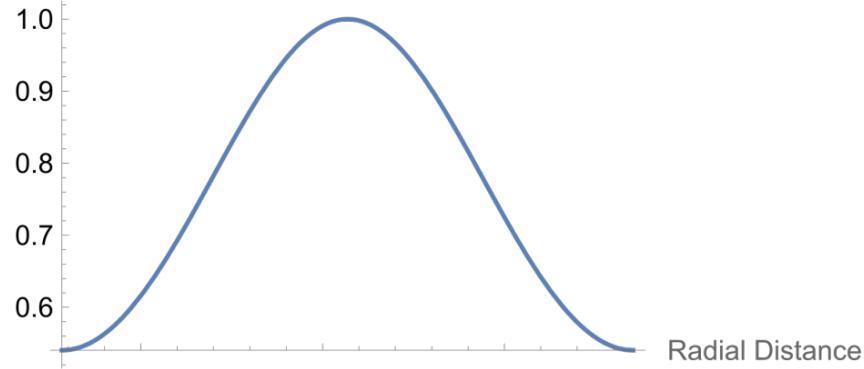 Fig. 12: Nodal- and Antinodal Regions for Standing (Confined) Electromagnetic within two concentric spheres. Equation (18) ## V. UNIVERSAL EQUILIBRIUM IN THE "CONCEPT OF QUANTUM MECHANICAL PROBABILITY" IN "THE NEW THEORY" The 4-dimensional notation for the divergence of the Stress-Energy Tensor (25) expresses in the 4th dimension (time dimension) the law of Conservation of Energy". For an Electromagnetic Field the law for conservation of Energy has been expressed as: $$ \overline {{f}} ^ {4} = \left( \begin{array}{c} f _ {4} \\f _ {3} \\f _ {2} \\f _ {1} \end{array} \right) = \square \square \overline {{\overline {{\mathbf {T}}}}} = \left( \begin{array}{c} \nabla . \overline {{\mathbf {S}}} + \frac {\partial \mathbf {w}}{\partial t} \\f _ {3} \\f _ {2} \\f _ {1} \end{array} \right) \quad = \overline {{0}} ^ {4} \tag {29} $$ The process of deriving the "Fundamental Equation for Confined Electromagnetic Interaction" in the proposed theory from the equation for the "Conservation of Electromagnetic Energy" (38.1) leads to a significant revelation. This fundamental equation serves as the cornerstone of the theory, resembling the Relativistic Quantum Mechanical "Dirac" equation and the Schrödinger wave equation, particularly when dealing with velocities significantly lower than the speed of light. In essence, this "Fundamental Equation for Confined Electromagnetic Interaction" can be viewed as the relativistic counterpart to the Quantum Mechanical Schrödinger wave equation, aligning closely with the Quantum Mechanical Dirac Equation. This unification and connection between these fundamental equations shed light on the intricate relationship between electromagnetic interactions, quantum mechanics, and relativistic dynamics within the proposed theoretical framework. ### a) Confined Electromagnetic Energy within a 4-dimensional Equilibrium The physical concept of quantum mechanical probability waves has been created during the famous 1927 5th Solvay Conference. During that period there were several circumstances which came just together and made it possible to create a unique idea of "Material Waves"(Solutions of Schödinger's wave equation) being complex (partly real and partly imaginary) and describing the probability of the appearance of a physical object (elementary particle) generally indicated as "Quantum Mechanical Probability Waves". The idea of complex (probability) waves is directly related to the concept of confined (standing) waves. Characteristic for any standing acoustical wave is the fact that the Velocity and the Pressure (Electric Field and Magnetic Field in QLT) are always shifted over 90 degrees. The same principle does exist for the standing (confined) electromagnetic waves, For that reason every confined (standing) electromagnetic wave can be described by a complex sum vector $\bar{\phi}$ of the Electric Field Vector $\overline{\mathbf{E}}$ and the Magnetic Field Vector $\overline{\mathbf{B}}$ ( $\overline{\mathbf{E}}$ has 90 degrees phase shift compared to $\overline{\mathbf{B}}$ ). The vector functions $\bar{\phi}$ and the complex conjugated vector function $\bar{\phi}^*$ will be written as: $$ \bar {\phi} = \frac {1}{\sqrt {2 \mu}} \left(\bar {\mathrm {B}} + \mathrm {i} \frac {\bar {\mathrm {E}}}{c}\right) \tag {30} $$ $\overline{\mathbf{B}}$ equals the magnetic induction, $\overline{\mathbf{E}}$ the electric field intensity ( $\overline{\mathbf{E}}$ has + 90 degrees phase shift compared to $\overline{\mathbf{B}}$ ) and c the speed of light. The complex conjugated vector function $\overline{\phi^{*}}$ equals: $$ \overline {{\phi^ {*}}} = \frac {1}{\sqrt {2 \mu}} \left(\bar {\mathrm {B}} - \mathrm {i} \frac {\bar {\mathrm {E}}}{c}\right) \tag {31} $$ The dot product equals the electromagnetic energy density w: $$ \bar {\phi}. \bar {\phi} ^ {*} = \frac {1}{2 \mu} \left(\bar {\mathrm {B}} + \mathrm {i} \frac {\bar {\mathrm {E}}}{c}\right). \left(\bar {\mathrm {B}} - \mathrm {i} \frac {\bar {\mathrm {E}}}{c}\right) = \frac {1}{2} \mu \mathrm {H} ^ {2} + \frac {1}{2} \varepsilon \mathrm {E} ^ {2} = \mathrm {w} \tag {32} $$ Using Einstein's equation $W = m c^2$, the dot product equals the electromagnetic mass density $w$: $$ \bar{\phi} \cdot \bar{\phi}^* \frac{1}{c^2} = \frac{\varepsilon}{2} \left(\bar{B} + i \frac{\bar{E}}{c}\right) \cdot \left(\bar{B} - i \frac{\bar{E}}{c}\right) = \frac{1}{\varepsilon} \varepsilon \mu^2 H^2 + \frac{1}{2} \varepsilon^2 E^2 = \rho \left[\mathrm{kg}/\mathrm{m}^3\right] $$ The cross product is proportional to the Poynting vector (Ref. 3, page 202, equation 15). $$ \bar{\phi} \times \bar{\phi}^* = \frac{1}{2\mu} \left(\bar{\mathrm{B}} + \mathrm{i} \frac{\bar{\mathrm{E}}}{c}\right) \times \left(\bar{\mathrm{B}} - \mathrm{i} \frac{\bar{\mathrm{E}}}{c}\right) = \mathrm{i} \sqrt{\varepsilon \mu} \quad \bar{\mathrm{E}} \times \bar{\mathrm{H}} = \mathrm{i} \sqrt{\varepsilon \mu} \quad \bar{\mathrm{S}} \tag{34} $$ Within this article, a novel "Gravitational-Electromagnetic Equation" is put forth, offering a detailed description of Electromagnetic Field Configurations. These configurations not only serve as mathematical solutions for the Scalar Quantum Mechanical "Schrodinger Wave Equation" but also, more precisely, correspond to the mathematical solutions encapsulated in the Tensor representation of the "Relativistic Quantum Mechanical Dirac Equation" (Equation 41). By establishing this linkage between the Gravitational-Electromagnetic Equation and the fundamental equations of Quantum Mechanics, specifically the Schrödinger Wave Equation and the Dirac Equation, the article outlines a comprehensive framework that integrates gravitational and electromagnetic interactions within the context of relativistic quantum mechanics. This synthesis of concepts aims to provide a deeper understanding of the dynamics governing electromagnetic fields and their connections to quantum mechanical phenomena at a relativistic scale. The 4-dimensional divergence of the sum of the Electromagnetic Stress-Energy tensor expresses the 4-dimensional Force-Density vector (expressed in $\left[\mathrm{N} / \mathrm{m}^{3}\right]$ in the 3 spatial coordinates) as the result of Electro-Magnetic-Gravitational interaction. $$ f ^ {\mu} = \partial_ {v} T ^ {\mu v} = 0 \tag {35} $$ In vector notation the 4-dimensional Force-Density vector can be written as: $$ \overline {{f}} ^ {4} = \left( \begin{array}{l} f _ {4} \\f _ {3} \\f _ {2} \\f _ {1} \end{array} \right) = \square \square \overline {{\overline {{\mathbf {T}}}}} = 0 \tag {36} $$ The pivotal boundary condition in this alternative gravitational approach necessitates that the Force 4-vector equals zero across the 4 dimensions, reflecting a universal equilibrium within the multidimensional framework. The spatial components of the Force-Density vector, arising from the intricate interplay of Electro-Magnetic-Gravitational interactions, can be explicitly articulated. By integrating the specific electromagnetic values for the electric field intensity "E" and the magnetic field intensity "H" into the formulation described in equation (36), the resulting expression encapsulates the 4-dimensional manifestation of the Electro-Magnetic-Gravitational Fields Equation (37). This amalgamation of electromagnetic and gravitational fields within the 4-dimensional realm underscores the comprehensive nature of the proposed framework and its implications for understanding the interactions between these fundamental forces. #### Energy-Time Domain $$ \left(\mathrm{f}_{4}\right)\Leftrightarrow\nabla\cdot\left(\overline{\mathrm{E}}\times\overline{\mathrm{H}}\right)+\frac{1}{2}\frac{\partial\left(\varepsilon_{0}\left(\overline{\mathrm{E}}\cdot\overline{\mathrm{E}}\right)+\mu_{0}\left(\overline{\mathrm{H}}\cdot\overline{\mathrm{H}}\right)\right)}{\partial t}=0 $$ #### 3-Dimensional Space Domain $$ \begin{array}{l} \left( \begin{array}{c} \mathrm{f}_{3} \\\mathrm{f}_{2} \\\mathrm{f}_{1} \end{array} \right) \Leftrightarrow \frac{1}{c^{2}} \frac{\partial (\overline{\mathrm{E}} \times \overline{\mathrm{H}})}{\partial t} + \varepsilon_{0} \overline{\mathrm{E}} \left(\nabla \cdot \overline{\mathrm{E}}\right) - \varepsilon_{0} \overline{\mathrm{E}} \times \left(\nabla \times \overline{\mathrm{E}}\right) \\+ \mu_{0} \overline{\mathrm{H}} \left(\nabla \cdot \overline{\mathrm{H}}\right) - \mu_{0} \overline{\mathrm{H}} \times \left(\nabla \times \overline{\mathrm{H}}\right) = \overline{0} \tag{37} \\\end{array} $$ In which $f_1$, $f_2$, $f_3$, represent the force densities in the 3 spatial dimensions and $f_4$ represent the force density (energy flow) in the time dimension ( $4^{\text{th}}$ dimension). Equation (37) can be written as: #### Energy-Time Domain #### Conservation of Energy $$ \left(\mathrm {f} _ {4}\right) \quad \begin{array}{l} \text {B - 7} \\\nabla . \bar {\mathrm {S}} + \frac {\partial \mathrm {w}}{\partial t} = 0 \end{array} \tag {38.1} $$ #### 3-Dimensional Space Domain $$ \left( \begin{array}{l l} \mathrm{f}_{3} & - \frac{1}{c^{2}} \frac{\partial (\bar{\mathrm{E}} \times \bar{\mathrm{H}})}{\partial t} + \varepsilon_{0} \bar{\mathrm{E}} (\nabla \cdot \bar{\mathrm{E}}) - \varepsilon_{0} \bar{\mathrm{E}} \times (\nabla \times \bar{\mathrm{E}}) + \\\mathrm{f}_{2} & \mathrm{f}_{1} \\& \end{array} \right) \quad \begin{array}{l l} \mathrm{B} - 1 & \mathrm{B} - 2 \\\mathrm{B} - 4 & \mathrm{B} - 5 \\+ \mu_{0} \bar{\mathrm{H}} (\nabla \cdot \bar{\mathrm{H}}) - \mu_{0} \bar{\mathrm{H}} \times (\nabla \times \bar{\mathrm{H}}) = \bar{0} \end{array} \tag{38} $$ The $4^{\text{th}}$ term in equation (38.1) can be written in the terms of the Poynting vector "S" and the energy density "w" representing the electromagnetic law for the conservation of energy (Newton's second law of motion). ### b) The 4-dimensional Relativistic Dirac Equation Substituting (32) and (34) in Equation (38.1) results in The 4-Dimensional Tensor presentation for the relativistic quantum mechanical Dirac Equation (39): $$ \left(\mathrm{x}_{4}\right)\quad \nabla\cdot\left(\bar{\phi}\times\overline{\phi^{*}}\right)\, +\, \frac{i}{c}\frac{\partial\bar{\phi}\cdot\bar{\phi}^{*}}{\partial t}\, =\, 0 $$ $$ \left( \begin{array}{l} \mathrm{x}_{3} \\\mathrm{x}_{2} \\\mathrm{x}_{1} \end{array} \right) \frac{i}{c} \frac{\partial (\bar{\phi} \times \bar{\phi}^{*})}{\partial t} - \left( \bar{\phi} \times (\nabla \times \bar{\phi}^{*}) + \bar{\phi}^{*} \times (\nabla \times \bar{\phi}) \right) + \left( \bar{\phi} (\nabla \cdot \bar{\phi}^{*}) + \bar{\phi}^{*} (\nabla \cdot \bar{\phi}) \right) = 0 \tag{39} $$ To transform the electromagnetic vector wave function $\overline{\phi}$ into a scalar (spinor or one-dimensional matrix representation), the Pauli spin matrices $\sigma$ and the following matrices (Ref. 3 page 213, equation 99) are introduced: $$ \bar{\alpha} = \left[ \begin{array}{l l} 0 & \sigma \\\sigma & 0 \end{array} \right] \quad \text{and} \quad \bar{\beta} = \left[ \begin{array}{c c} \delta_ {a b} & 0 \\0 & - \delta_ {a b} \end{array} \right] \tag{40} $$ The Equations(6), (32) and (34) can be written in tensor presentation as the 4-Dimensional Relativistic Quantum Mechanical Dirac Equation: [3](Equation 102, page 213) $$ \left(\mathrm{x}_{4}\right)\quad\left(\frac{\mathrm{im}\,c}{h}\,\bar{\beta}+\bar{\alpha}\cdot\nabla\right)\psi=-\frac{1}{c}\frac{\partial\psi}{\partial t}\tag{41.1} $$ $$ \left(\begin{array}{l}\mathrm{x}_{3}\\\mathrm{x}_{2}\\\mathrm{x}_{1}\end{array}\right)\quad -\frac{1}{c^{2}}\frac{\partial(\overline{\mathrm{E}}\times\overline{\mathrm{H}})}{\partial t}+\varepsilon_{0}\overline{\mathrm{E}}\left(\nabla\cdot\overline{\mathrm{E}}\right)-\varepsilon_{0}\overline{\mathrm{E}}\times\left(\nabla\times\overline{\mathrm{E}}\right)+\mu_{0}\overline{\mathrm{H}}\left(\nabla\cdot\overline{\mathrm{H}}\right)-\mu_{0}\overline{\mathrm{H}}\times\left(\nabla\times\overline{\mathrm{H}}\right)+\gamma_{0}\overline{\mathrm{g}}\left(\nabla\cdot\overline{\mathrm{g}}\right)-\gamma_{0}\overline{\mathrm{g}}\times\left(\nabla\times\overline{\mathrm{g}}\right)=0\tag{41} $$ ## VI. HEISENBERG'S UNCERTAINTY RELATIONSHIP # a) The Inertia of Confined Electromagnetic Radiation According to the insights derived from equation (23), the solutions of the Schrödinger wave equation depict confined electromagnetic waves characterized by a distinct 90-degree phase shift between the electric and magnetic fields. This segment delves into exploring the concept of inertia associated with confined electromagnetic waves. To elucidate the calculation of inertia pertaining to confined electromagnetic radiation, a hypothetical scenario involving electromagnetic radiation trapped between two perfectly reflective mirrors will be considered. The radiation beams emanating from these mirrors, referred to as the emitted radiation, can be likened to light emitted from a source of electromagnetic radiation. In this scenario, when an observer moves towards the emitter, the intensity of light at the observer's position undergoes a transformation in accordance with the Lorentz transformation formula, where "v" signifies the relative velocity between the emitter and the observer. At relatively low velocities, the term in the Lorentz transformation equation simplifies to 1, reflecting the behavior observed in this regime. When the observer moves away from the emitter, the intensity of the light at the location of the observer will decrease with $\gamma (1 - \nu /c)$ according the Lorentz transformation. At low velocities the Lorentz contraction term: $$ \gamma = \frac {1}{\sqrt {1 - \frac {\mathrm {v} ^ {2}}{\mathrm {c} ^ {2}}}} \tag {42} $$ will equal 1 ("v" equals the relative velocity between object and observer and c equals the speed of light). In the scenario where light is confined between two perfectly reflective mirrors, a significant observation emerges: the speeds of both mirrors remain consistently equal relative to each other. This equilibrium ensures that the radiation pressures exerted on each mirror are also in balance; these opposing radiation pressures effectively cancel each other out. Consequently, the system—comprising the two perfect mirrors and the confined electromagnetic radiation—will either remain at rest or continue moving at a uniform speed. This dynamic equilibrium underscores the intricate interplay between the confined electromagnetic radiation and the reflective surfaces in this conceptual framework. ## i. The Resulting Radiation Pressure for accelerated or decelerated confined electromagnetic radiation In the context of acceleration, an interesting phenomenon arises where the time taken for light to travel between the mirrors at the speed of light can introduce variations. If we designate one mirror as the emitter and the other as the observer, the apparent speeds of the emitter and observer differ due to the time delay inherent in light propagation during acceleration. This time discrepancy gives rise to a situation where the opposing radiation pressures on the mirrors are no longer balanced, leading to an imbalance in forces. This disparity in radiation pressures may engender a resultant force as per Newton's second law of motion during acceleration. To embark on this analysis, an imaginary experiment is envisioned. Two perfectly reflective mirrors, labeled as B and A and situated opposite each other in the x-y plane at a specific distance, serve as the setting. Within this framework, a single harmonic electromagnetic wave is confined between the mirrors, giving rise to a "Standing Electromagnetic Wave" akin to the solution described in equation (23). This standing wave configuration is the outcome of two waves propagating in opposite directions along the $z$ -axis, underpinning the dynamics of this experimental scenario. The Poynting vector corresponding with the electromagnetic wave propagating along the $z$ -axis in the $+$ direction (positive direction of the $z$ -axis) has been indicated as $\overline{\mathbf{S}}^{+} = \overline{\mathbf{E}}^{+} \times \overline{\mathbf{H}}^{+}$ and the Poynting vector corresponding with the electromagnetic wave propagating along the $z$ -axis in the - direction (opposite direction) has been indicated as $\overline{\mathbf{S}}^{-} = \overline{\mathbf{E}}^{-} \times \overline{\mathbf{H}}^{-}$. The system is at rest. The radiation pressures, caused by the confined electromagnetic radiation, on both mirrors A and B are opposite and equal in magnitude: $$ \mathbf{P}_{\mathrm{A}} = \frac{2 \mathbf{S}_{\mathrm{A}}}{\mathbf{c}} = \frac{2 \mathbf{S}_{\mathrm{B}}}{\mathbf{c}} = \mathbf{P}_{\mathrm{B}} \tag{43} $$ To calculate the radiation pressure on Mirror A, the velocities, only relative to Mirror A for the waves with the respective Poynting vectors $\overline{S}^{+} = \overline{E}^{+}\times \overline{H}^{+}$ and $\overline{S}^{-} = \overline{E}^{-}\times \overline{H}^{-}$, have to be calculated. ii. The radiation pressure on Mirror A, when Mirror A moves with a velocity $v$ in the direction of the positive $z$ -axis When the system of two Mirrors "B - A" moves in the direction of the positive $z$ -axis, Mirror A moves in the direction of the positive $z$ -axis and the Poynting vector for the emitted radiation $\overline{S}^{+} = \overline{E}^{+} \times \overline{H}^{+}$ will decrease according to the Lorentz transformation. $$ \overline {{S}} _ {\mathrm {v}} ^ {+} = \overline {{\mathbf {E}}} _ {\mathrm {v}} ^ {+} \times \overline {{\mathbf {H}}} _ {\mathrm {v}} ^ {+} = \gamma^ {2} \left(1 - \frac {\mathrm {v}}{\mathrm {c}}\right) ^ {2} \left(\overline {{\mathbf {E}}} ^ {+} \times \overline {{\mathbf {H}}} ^ {+}\right) \tag {44} $$ When the system of two Mirrors "B - A" moves in the direction of the positive $z$ -axis, Mirror A moves in the direction of the positive $z$ -axis. The Poynting vector for the incident radiation $\overline{S}^{-} = \overline{E}^{-} \times \overline{H}^{-}$ will increase according to the Lorentz transformation. $$ \bar {S} _ {\mathrm {v}} ^ {-} = \bar {\mathrm {E}} _ {\mathrm {v}} ^ {-} \times \bar {\mathrm {H}} _ {\mathrm {v}} ^ {-} = \gamma^ {2} \left(1 + \frac {\mathrm {v}}{\mathrm {c}}\right) ^ {2} \left(\bar {\mathrm {E}} ^ {+} \times \bar {\mathrm {H}} ^ {+}\right) \tag {45} $$ The total radiation pressure, caused by the confined electromagnetic radiation, on mirror A equals: $$ \mathrm {P} _ {\mathrm {A}} = \frac {\mathrm {S} _ {A} ^ {+} + \mathrm {S} _ {A} ^ {-}}{\mathrm {c}} = \frac {\gamma^ {2} \left(\left(1 - \frac {\mathrm {v}}{\mathrm {c}}\right) ^ {2} + \left(1 + \frac {\mathrm {v}}{\mathrm {c}}\right) ^ {2}\right) \left(\overline {{\mathrm {E}}} ^ {+} \times \overline {{\mathrm {H}}} ^ {+}\right)}{\mathrm {c}} \tag {46} $$ iii. The radiation pressure on Mirror B when Mirror B moves with a velocity $v$ in the direction of the positive $z$ -axis When the system of two Mirrors "B – A" moves in the direction of the positive z-axis, Mirror B moves in the direction of the positive z-axis and the Poynting vector for the by mirror "B" emitted radiation will increase according the Lorentz transformation. $$ \bar {S} _ {\mathrm {v}} ^ {-} = \bar {\mathrm {E}} _ {\mathrm {v}} ^ {-} \times \bar {\mathrm {H}} _ {\mathrm {v}} ^ {-} = \gamma^ {2} \left(1 + \frac {\mathrm {v}}{\mathrm {c}}\right) ^ {2} \left(\bar {\mathrm {E}} ^ {+} \times \bar {\mathrm {H}} ^ {+}\right) \tag {47} $$ When the system of two Mirrors "B - A" moves in the direction of the positive z-axis, Mirror B moves in the direction of the positive z-axis the Poynting vector for the on mirror B incident radiation $\overline{\mathbf{S}}^{+} = \overline{\mathbf{E}}^{+}\times \overline{\mathbf{H}}^{+}$ will decrease according the Lorentz transformation. $$ \overline {{S}} _ {\mathrm {v}} ^ {+} = \overline {{\mathbf {E}}} _ {\mathrm {v}} ^ {+} \times \overline {{\mathbf {H}}} _ {\mathrm {v}} ^ {+} = \gamma^ {2} \left(1 - \frac {\mathrm {v}}{\mathrm {c}}\right) ^ {2} \left(\overline {{\mathbf {E}}} ^ {+} \times \overline {{\mathbf {H}}} ^ {+}\right) \tag {48} $$ The total radiation pressure, caused by the confined electromagnetic radiation, on mirror B equals: $$ P _ {B} = \frac {S _ {B} ^ {+}}{c} + _ {B} ^ {-} S = \frac {\gamma^ {2} \left(\left(1 + \frac {v}{c}\right) ^ {2} + \left(1 - \frac {v}{c}\right) ^ {2}\right) \left(\overline {{E}} ^ {+} \times \overline {{H}} ^ {+}\right)}{c} \tag {49} $$ $\mathsf{P}_{\mathrm{A}}$ and $\mathsf{P}_{\mathrm{B}}$ are still equal in magnitude and both in opposite direction and still cancel each other. The system of confined radiation validates Newton's first law of motion. ## iv. Newton's second Law of Motion (Inertia) for Confined Electromagnetic Radiation When the system of two Mirrors "B - A" accelerates, the velocity increases with $\Delta \mathbf{v}$ in a time interval $\Delta t$. At time "t" the opposite radiation pressures on mirror A and mirror B are presented in (46) and (49). At time $t + \Delta t$ the radiation pressures on Mirror A and Mirror B will differ. The radiation pressure at time $t + \Delta t$ caused by the confined electromagnetic radiation, on mirror A equals: $$ P _ {A} = \frac {S _ {A} ^ {+} + S _ {A} ^ {-}}{c} = \frac {\gamma^ {2} \left(\left(1 + \frac {(v)}{c}\right) ^ {2} + \left(1 - \frac {(v + \Delta v)}{c}\right) ^ {2}\right) \left(\overline {{E}} ^ {+} \times \overline {{H}} ^ {+}\right)}{c} \tag {50} $$ Because the electromagnetic wave with Poynting vector $\overline{\mathbf{S}}^{+} = \overline{\mathbf{E}}^{+}\times \overline{\mathbf{H}}^{+}$ has left Mirror B at "t" and during the time interval $\Delta t$ the magnitude of $\overline{\mathbf{E}}_{\mathrm{t}}^{+} = \left(1 + \frac{\mathbf{V}}{\mathbf{c}}\right)\overline{\mathbf{E}}^{+}$ and $\overline{\mathbf{H}}_{\mathrm{t}}^{+} = \left(1 + \frac{\mathbf{V}}{\mathbf{c}}\right)\overline{\mathbf{H}}^{+}$ has not changed. The radiation pressure at time $t + \Delta t$ caused by the confined electromagnetic radiation, on mirror B equals: $$ \mathrm {P} _ {B} = \frac {\mathrm {S} _ {B} ^ {+} + \mathrm {S} _ {B} ^ {-}}{\mathrm {c}} = \frac {\gamma^ {2} \left(\left(1 + \frac {(\mathrm {v} + \Delta \mathrm {v})}{\mathrm {c}}\right) ^ {2} + \left(1 - \frac {(\mathrm {v})}{\mathrm {c}}\right) ^ {2}\right) \left(\overline {{\mathrm {E}}} ^ {+} \times \overline {{\mathrm {H}}} ^ {+}\right)}{\mathrm {c}} \tag {51} $$ Because the wave with Poynting vector $\overline{S}^{-} = \overline{\mathbf{E}}^{-}\times \overline{\mathbf{H}}^{-}$ has left Mirror A at "t" and during the time interval $\pmb{\Delta}$ t the magnitude of $\overline{\mathbf{E}}_{\mathrm{t}}^{-} = \left(1 + \frac{\mathrm{v}}{\mathrm{c}}\right)\overline{\mathbf{E}}^{-}$ and $\overline{\mathbf{H}}_{\mathrm{t}}^{-} = \left(1 + \frac{\mathrm{v}}{\mathrm{c}}\right)\overline{\mathbf{H}}^{-}$ has not changed. The radiation pressures on Mirror A and Mirror B do not counterbalance each other anymore and the resulting radiation pressure equals: $$ \mathrm {P} _ {\mathrm {B}} - \mathrm {P} _ {\mathrm {A}} = \frac {\gamma^ {2} (4 \Delta \mathrm {v}) \mathrm {S}}{\mathrm {c} ^ {2}} \tag {52} $$ Equation (52) can be written as: $$ P _ {B} - P _ {A} = \frac {\gamma^ {2} (4 \Delta v) S}{c ^ {2}} = \frac {\gamma^ {2} \left(4 \frac {\Delta v}{\Delta t}\right) S \Delta t}{c ^ {2}} = \gamma^ {2} \left(\frac {W}{c ^ {2}}\right) a = \gamma^ {2} m a \tag {53} $$ In which the acceleration $\mathbf{a} = \frac{\Delta \mathbf{v}}{\Delta t}$ and the inertia $\mathbf{m} = \frac{\mathbf{W}}{c^2}$. At non-relativistic velocities $\gamma = 1$ and (53) validates Newton's second law of motion for confined electromagnetic radiation presented in equation (23). According Einstein's $\mathbf{W} = \mathbf{m} \mathbf{c}^2$ the confined electromagnetic energy "W" equals the total confined electromagnetic mass. By superposition and integration over arbitrary surfaces it is possible to prove that all confined electromagnetic radiation equals (53) which represents that confined electromagnetic energy validates Newton's second law of motion ( $F = ma$ ). ### b) Heisenberg's Uncertainty Relationship For confined electromagnetic radiation represented in (23) the mass has been represented in (53). According Planck's law the energy "W" is proportional to the frequency of the confined electromagnetic radiation: $$ \mathrm {W} = \hbar \mathrm {f} $$ $$ \mathbf {W} = \mathbf {m} \mathbf {c} ^ {2} = \hbar \mathbf {f} \tag {54} $$ Both sides in equation (54) are multiplied by the velocity of the confined electromagnetic radiation. $$ (m v) c ^ {2} = \hbar f v $$ $$ p = \frac {\hbar f v}{c ^ {2}} \tag {55} $$ Resulting in an expression for the momentum "p" of the confined radiation. According Planck a variation in the momentum "p" will result in the variation of the frequency "f" of the confined electromagnetic radiation. $$ \Delta \mathrm {p} = \frac {\hbar (\Delta) ^ {\mathrm {f}}}{\mathrm {c} ^ {2}} \quad \mathrm {v} \tag {56} $$ Because of the relationship between the frequency "f" and the wavelength $\lambda$ (56) can be written as: $$ \Delta \mathrm {p} = \left(\frac {\hbar \Delta \mathrm {f}}{\mathrm {c} ^ {2}}\right) \mathrm {v} $$ $$ \Delta \mathrm {p} = \left(\frac {\hbar}{\mathrm {c} \Delta \lambda}\right) \mathrm {v} \tag {57} $$ Presenting confined electromagnetic radiation, equation (57) can be written in a way comparable with Heisenberg's uncertainty relationship: $$ \left(\Delta \lambda \Delta \mathrm {p}\right) = \hbar \left(\frac {\mathrm {v}}{\mathrm {c}}\right) \tag {58} $$ For uniform moving electromagnetic confinements the velocity "v" remains constant and the product of the uncertainty in the wavelength (dimension of the confinement) and the uncertainty in the momentum (frequency) of the confinement represents a constant value. It follows from equation (58) there is no fundamental uncertainty. Heisenberg's "Uncertainty Relationship" represents the constant relationship between the wavelength (dimension) and the frequency (momentum) for gravitationally confined light and in general gravitationally confined electromagnetic waves. ## VII. CONCLUSIONS The integration of General Relativity with the new proposed theory provides a fascinating perspective on the interaction between gravity and light within a 4-dimensional spacetime curvature defined by a gravitational field. In this framework, light's trajectory is dictated by the curved spacetime geometry, illustrating the profound relationship between gravity and electromagnetic phenomena. The new theory introduces a novel concept of bi-directional separation between mass and inertia for light, specifically photons. In this view, inertia is exclusively present in the direction of light propagation, influencing the speed of light. On the other hand, mass of light exists in a plane perpendicular to the propagation direction, affecting the deflection of light by gravitational fields perpendicular to the propagation. This distinction sheds light on the nuanced dynamics of light-matter interactions within gravitational fields. Black Holes, as gravitational-electromagnetic confinements, are fundamental solutions derived from the relativistic quantum mechanical Dirac equation. These enigmatic cosmic entities highlight the significant gravitational intensity shift and redshift induced by gravitational fields. The impact of "CURL" within gravitational fields surrounding Black Holes remains a distinctive feature that challenges conventional explanations afforded by General Relativity. By considering a 4-dimensional equilibrium encompassing inertia and gravitational force densities within electromagnetic field configurations, the theory presents Black Holes as physical entities at sub-atomic scales. These solutions exhibit spherical confinements with discrete energy levels, offering a unique perspective on the quantum nature of these phenomena. In experimental validation, the theory proposes measuring the interaction between gravity and light in well-defined gravitational fields, such as that of Earth. Discrepancies in gravitational redshift calculations between General Relativity and the new theory, albeit minuscule, underscore the need for higher accuracy observations to discern between the two frameworks effectively. Dark Matter's existence is postulated based on gravitational redshift and gravitational intensity shift phenomena. The concept of "Gravitational Shielding" elucidates how entire galaxies, with immense mass, may become invisible due to gravitational effects, even with advanced observatories like the James Webb Space Telescope. This invisibility beyond a certain distance poses intriguing challenges for observational astronomy and underscores the mysterious nature of dark matter within our universe. Lastly, equation (58) within the theory establishes a clear relationship without fundamental uncertainty. Heisenberg's Uncertainty Principle is redefined in the context of gravitationally confined light, presenting a constant relationship between wavelength and frequency for electromagnetic waves in such settings. ### a) Data Availability All Data and Calculations have been published at: https://quantumlight.science/

Generating HTML Viewer...

References

38 Cites in Article
John Wheeler,; Archibald,Geons (1955). Geons.
Sven Herrmann,Felix Finke,Martin Lülf,Olga Kichakova,Dirk Puetzfeld,Daniela Knickmann,Meike List,Benny Rievers,Gabriele Giorgi,Christoph Günther,Hansjörg Dittus,Roberto Prieto-Cerdeira,Florian Dilssner,Francisco Gonzalez,Erik Schönemann,Javier Ventura-Traveset,Claus Lämmerzahl (2018). Test of the Gravitational Redshift with<i>Galileo</i>Satellites in an Eccentric Orbit.
J Vegt (1995). A Continuous Model of Matter based on AEONs.
(2004). Quantum theory and light propagation.
A Godone,C Novero,P Tavella (1995). Null gravitational redshift experiment with nonidentical atomic clocks.
Pavel Korobkov (null). General relativistic theory of light propagation in the field of gravitational multipoles.
Raymond Beach (2014). A Classical Field Theory of Gravity and Electromagnetism.
James Maxwell,Clerk (1865). A dynamical theory of the electromagnetic field.
A Einstein (1911). Über den Einfluß der Schwerkraft auf die Ausbreitung des Lichtes.
Mahendra Goray,Ramesh Annavarapu (2020). Rest mass of photon on the surface of matter.
A Genova,E Mazarico,S Goossens (2018). Solar system expansion and strong equivalence principle as seen by the NASA MESSENGER mission.
John Williamson (2019). A new linear theory of light and matter.
D Sciama (1964). The Physical Structure of General Relativity.
Adrian Del Rio,Jose Navarro-Salas,Francisco Torrenti (2014). Renormalized stress-energy tensor for spin-<mml:math xmlns:mml="http://www.w3.org/1998/Math/MathML" display="inline"><mml:mrow><mml:mn>1</mml:mn><mml:mo>/</mml:mo><mml:mn>2</mml:mn></mml:mrow></mml:math>fields in expanding universes.
Stergios Pellis (2023). Unity Formulas for the Coupling Constants and the Dimensionless Physical Constants.
Yakov Bloch,Joshua Foo (2023). How the result of a measurement of a photon's mass can turn out to be 100.
Arámburo Andrés,Kyrylo García,Sylvia Bondarenko,Josef Ploeckinger,Anastasia Pradler,Sokolenko (2020). Effective photon mass and (dark) photon conversion in the inhomogeneous Universe.
M Alexander,Nadezhda Gabovich,Gabovich (2007). How to explain the non-zero mass of electromagnetic radiation consisting of zero-mass photons.
Liang-Cheng Tu,Jun Luo,George Gillies (2004). The mass of the photon.
B Doyon (2013). Conformal Loop Ensembles and the Stress-Energy Tensor.
Thomas-Paul Hack,Valter Moretti (2012). On the stress–energy tensor of quantum fields in curved spacetimes—comparison of different regularization schemes and symmetry of the Hadamard/Seeley–DeWitt coefficients.
Adam Levi (2017). Renormalized stress-energy tensor for stationary black holes.
Julio Gobbi (Dece). Unknown Title.
Xing-Hao Ye,Qiang Lin (2008). Gravitational Lensing Analyzed by Graded Refractive Index of Vacuum.
Wim Vegt (2022). The Origin of Gravity in “Quantum Light Theory”..
P Delva,N Puchades,E Schönemann,F Dilssner,C Courde,S Bertone,F Gonzalez,A Hees,C Le Poncin-Lafitte,F Meynadier,R Prieto-Cerdeira,B Sohet,J Ventura-Traveset,P Wolf (2018). Gravitational Redshift Test Using Eccentric <i>Galileo</i> Satellites.
Jonathan Oppenheim (2023). A Postquantum Theory of Classical Gravity?.
Wim Vegt (2022). The Origin of Gravity, A second order Lorentz Transformation for “Accelerated Electromagnetic Fields”, Generating a Gravitational Field and the property of Mass.
Wim Vegt (2021). The 4-Dimensional Dirac Equation in Relativistic Field Theory.
Wim Vegt A Perfect Equilibrium inside a Black Hole.
Albert Einstein (2011). Elementare Uberlegungenzur Interpretation der Grundlagen der Quanten-Mechanik.
John Nikko,Leo Lobos,Reggie Pantig (2022). Generalized Extended Uncertainty Principle Black Holes: Shadow and lensing in the macro-and microscopic realms.
Zihua Weng (2008). Influence of velocity curl on conservation laws.
Explore published articles in an immersive Augmented Reality environment. Our platform converts research papers into interactive 3D books, allowing readers to view and interact with content using AR and VR compatible devices.
Your published article is automatically converted into a realistic 3D book. Flip through pages and read research papers in a more engaging and interactive format.
Our website is actively being updated, and changes may occur frequently. Please clear your browser cache if needed. For feedback or error reporting, please email [email protected]
Thank you for connecting with us. We will respond to you shortly.