I. INTRODUCTION

It is classically known that the normed algebra $C^0(X)$ of continuous real-valued functions on a compact space $X$ determines its topological type [GRS], [Ga], [Br]. In this context, $X$ is interpreted as the space of maximal ideals of the algebra $C^0(X)$. In a similar spirit, the algebra $C^{\mathrm{\infty }}(X)$ of smooth functions on a compact smooth manifold $X$ (the algebra $C^{\mathrm{\infty }}(X)$ is considered in the Whitney topology [W3]) determines the smooth topological type of $X$ [KMS], [Na]. Again, $X$ may be viewed as the space of maximal ideals of the algebra $C^{\mathrm{\infty }}(X)$.

Recall that a harmonic function $h$ on a compact connected Riemannian manifold $X$ is uniquely determined by its restriction to the smooth boundary $\partial X$ of $X$. In other words, the Dirichlet boundary value problem has a unique solution in the space of harmonic functions. Therefore, the vector space $\mathcal{H}(X)$ of harmonic functions on $X$ is rigidly determined by its restriction (trace) ${\mathcal{H}}^{\partial }(X):=\mathcal{H}(X){|}_{\partial X}$ to the boundary $\partial X$. As we embark on our journey, this fact will serve us as a beacon.

This paper revolves around the following question:

Which algebras of smooth functions on the boundary $\partial X$ can be used to reconstruct the algebra $C^{\mathrm{\infty }}(X)$ and thus the smooth topological type of $X$?

Remembering the flexible nature of smooth functions (in contrast with the rigid harmonic ones), at the first glance, we should anticipate the obvious answer "None!". However, when $X$ carries an additional geometric structure, then the question, surprisingly, may have a positive answer. The geometric structure on $X$ that does the trick is a vector field (i.e., an ordinary differential equation), drawn from a massive class of vector fields which we will introduce below.

Let $X$ be a compact connected smooth $(n+1)$ -dimensional manifold with boundary and $v$ a smooth vector field admitting a Lyapunov function $f:X\to \mathbb{R}$ so that . We call such vector fields traversing. We assume that $v$ is in general position with respect to the boundary $\partial X$ and call such vector fields boundary generic (see [K1] or [K3], Definition 5.1, for the notion of boundary generic vector fields). Temporarily, it will be sufficient to think of the boundary generic vector fields $v$ as having only $v$ -trajectories that are tangent to the boundary $\partial X$ with the order of tangency less than or equal to $\dim (X)$. Section 3 contains a more accurate definition.

Informally, we use the term "holography" when some residual structures on the boundary $\partial X$ are sufficient for a reconstruction of similar structures on the bulk $X$.

Given such a triple $(X,v,f)$, in Section 3, we will introduce two subalgebras, $\mathcal{A}(v)=C^{\mathrm{\infty }}(\partial X,v)$ and $\mathcal{B}(f)=(f^{\partial }{)}^{\ast }(C^{\mathrm{\infty }}(\mathbb{R}))$, of the algebra $C^{\mathrm{\infty }}(\partial X)$, which depend only on $v$ and $f$, respectively. By Theorem 3.1, $\mathcal{A}(v)$ and $\mathcal{B}(f)$ will allow for a reconstruction of the algebra $C^{\mathrm{\infty }}(X)$. In fact, the boundary data, generated by these subalgebras, lead to a unique (rigid) "solution"

the topological tensor product of the two algebras. As a result, the pair $\mathcal{A}(v),\mathcal{B}(f)$ "residing on the boundary", determines the smooth topological type of the bulk $X$ and of the 1-dimensional foliation $\mathcal{F}(v)$, generated by the $v$ -flow.

II. HOLEGRAPHY ON MANIFOLDS WITH BOUNDARY AND THE CAUSALITY MAPS

Let $X$ be a compact connected smooth $(n+1)$ -dimensional manifold with boundary ${\partial }_{1}X{=}_{\mathrm{def}}\partial X$ (we use this notation for the boundary $\partial X$ to get some consistency with similar notations below), and $v$ a smooth traversing vector field, admitting a smooth Lyapunov function $f:X\to \mathbb{R}$. We assume that $v$ is boundary generic.

We denote by ${\partial }_1^{+}X(v)$ the subset of ${\partial }_{1}X$ where $v$ is directed inwards of $X$ or is tangent to ${\partial }_{1}X$. Similarly, ${\partial }_1^{-}X(v)$ denotes the subset of ${\partial }_{1}X$ where $v$ is directed outwards of $X$ or is tangent to ${\partial }_{1}X$.

Let $\mathcal{F}(v)$ be the 1-dimensional oriented foliation, generated by the traversing $v$ -flow.

We denote by ${\gamma }_x$ the $v$ -trajectory through $x\in X$. Since $v$ is traversing and boundary generic, each ${\gamma }_x$ is homeomorphic either a closed segment, or to a singleton [K1].

In what follows, we embed the compact manifold $X$ in an open manifold $\hat{X}$ of the same dimension so that $v$ extends to a smooth vector field $\hat{v}$ on $\hat{X}$, $f$ extends to a smooth function $\hat{f}$ on $\hat{X}$, and in $\hat{X}$. We treat $(\hat{X},\hat{v},\hat{f})$ as a germ in the vicinity of $(X,v,f)$.

Definition 2.1. We say that a boundary generic and traversing vector field $v$ possesses Property A, if each $v$ -trajectory $\gamma$ is either transversal to ${\partial }_{1}X$ at some point of the set $\gamma \cap {\partial }_{1}X$, or $\gamma \cap {\partial }_{1}X$ is a singleton $x$ and $\gamma$ is quadratically tangent to ${\partial }_{1}X$ at $x$.

A traversing vector field $v$ on $X$ induces a structure of a partially-ordered set $({\partial }_{1}X,{\succ }_v)$ on the boundary ${\partial }_{1}X$: for $x,y\in {\partial }_{1}X$, we write $y\succ x$ if the two points lie on the same $v$ -trajectory $\gamma$ and $y$ is reachable from $x$ by moving in the $v$ -direction.

We denote by $\mathcal{T}(v)$ the trajectory space of $v$ and by $\mathrm{\Gamma }:X\to \mathcal{T}(v)$ the obvious projection. For a traversing and boundary generic $v$, $\mathcal{T}(v)$ is a compact space in the topology induced by $\mathrm{\Gamma }$. Since any trajectory of a traversing $v$ intersects the boundary ${\partial }_{1}X$, we get that $\mathcal{T}(v)$ is a quotient of ${\partial }_{1}X$ modulo the partial order relation ${\succ }_v$.

Figure 1: The map $\mathrm{\Gamma }:X\to \mathcal{T}(v)$ for a traversally generic (vertical) vector field $v$ on a disk with 4 holes. The trajectory space is a graph whose vertices are of valencies 1 and 3. The restriction of $\mathrm{\Gamma }$ to ${\partial }_{1}X$ is a surjective map ${\mathrm{\Gamma }}^{\partial }$ with finite fibers of cardinality 3 at most; a generic fiber has cardinality 2.

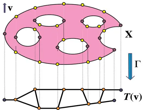
A traversing and boundary generic $v$ gives rise to the causality (scattering) map

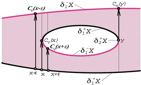
that takes each point $x\in {\partial }_1^{+}X(v)$ to the unique consecutive point $y\in {\gamma }_x\cap {\partial }_1^{-}X(v)$ that can be reached from $x$ in the $v$ -direction. If no such $y\ne x$ is available, we put $C_v(x)=x$. We stress that typically $C_v$ is a discontinuous map (see Fig. 2).

We notice that, for any smooth positive function $\lambda :X\to {\mathbb{R}}_{+}$, we have $C_{\lambda \cdot v}=C_v$; thus the causality map depends only on the conformal class of a traversing vector field $v$. In fact, $C_v$ depends only on the oriented foliation $\mathcal{F}(v)$, generated by the $v$ -flow.

In the paper, we will discuss two kinds of intimately related holography problems. The first kind amounts to the question: To what extend given boundary data are sufficient for reconstructing the unknown bulk and the traversing $v$ -flow on it, or rather, the foliation $\mathcal{F}(v)$? This question may be represented symbolically by the two diagrams:

Holographic Reconstruction Problem

Figure 2: An example of the causality map $C_v:{\partial }_1^{+}X(v)\to {\partial }_1^{-}X(v)$. Note the essential discontinuity of $C_v$ in the vicinity of $x$.

where ${\succ }_v$ denotes the partial order on boundary, defined by the causality map $C_v$, and the symbol " $\Rightarrow$ " points to the unknown ingredients of the diagrams.

The second kind of problem is: Given two manifolds, $X_1$ and $X_2$, equipped with traversing flows, and a diffeomorphism ${\mathrm{\Phi }}^{\partial }$ of their boundaries, respecting the relevant boundary data, is it possible to extend ${\mathrm{\Phi }}^{\partial }$ to a diffeomorphism/homeomorphism $\mathrm{\Phi }:X_1\to X_2$ that respects the corresponding flows-generated structures in the interiors of the two manifolds?

This problem may be represented by the commutative diagrams:

Holographic Extension Problem

where inc denotes the inclusion of spaces, accompanied by the obvious restrictions of functions and foliations. The symbol " $\downarrow$??" indicates the unknown maps in the diagrams.

These two types of problems come in a big variety of flavors, depending on the more or less rich boundary data and on the anticipated quality of the transformations $\mathrm{\Phi }$ (homeomorphisms, PD-homeomorphisms, Hölder homeomorphisms with some control of the Hölder exponent, and diffeomorphisms with different degree of smoothness).

Let us formulate the main result of [K4], Theorem 4.1, which captures the philosophy of this article and puts our main result, Theorem 3.1, in the proper context. Theorem 2.1 reflects the scheme depicted in (2.4).

Theorem 2.1. (Conjugate Holographic Extensions) Let $X_1,X_2$ be compact connected oriented smooth ( $n+1$ -dimensional manifolds with boundaries). Consider two traversing boundary generic vector fields $v_1,v_2$ on $X_1$ and $X_2$, respectively. In addition, assume that $v_1,v_2$ have Property A from Definition 2.1.

Let a smooth orientation-preserving diffeomorphism ${\mathrm{\Phi }}^{\partial }:{\partial }_1{X}_1\to {\partial }_1{X}_2$ commute with the two causality maps:

Then ${\mathrm{\Phi }}^{\partial }$ extends to a smooth orientation-preserving diffeomorphism $\mathrm{\Phi }:X_1\to X_2$ such that $\mathrm{\Phi }$ maps the oriented foliation $\mathcal{F}(v_1)$ to the oriented foliation $\mathcal{F}(v_2)$.

Let us outline the spirit of Theorem 2.1's proof, since this will clarify the main ideas from Section 3. The reader interested in the technicalities may consult [K4].

Proof. First, using that v_{2} is traversing, we construct a Lyapunov function f_{2}: X_{2} \to $\mathbb{R}$ for v_{2}. Then we pull-back, via the diffeomorphism \Phi^{\partial}, the restriction f_{2}^{\partial} \coloneqq f_{2}|{\partial{1}X_{2}} to the boundary ${\partial }_1$X_{2}. Since \Phi^{\partial} commutes with the two causality maps, the pull back f_{1}^{\partial} = {$\mathrm{def}$}(\Phi^{\partial} \circ f{2}^{\partial})(y) has the property f_{1}^{\partial}(y) > f_{1}^{\partial}(x) for any pair y > x on the same v_{1}-trajectory. Equivalently, we get f_{1}^{\partial}(C_{v_{1}}(x)) > f_{1}^{\partial}(x) for any x \in \partial_{1}^{+}X(v_{1}) such that C_{v_{1}}(x) \neq x. As the key step, we prove in [K4] that such f_{1}^{\partial} extends to a smooth function f_{1}: X_{1} \to $\mathbb{R}$ that has the property df_{1}(v_{1}) > 0. Hence, f_{1} is a Lyapunov function for v_{1}.

Recall that each causality map $C_{v_i}$, $i=1,2$, allows to view the $v_i$ -trajectory space $\mathcal{T}(v_i)$ as the quotient space $({\partial }_1{X}_i)/\{C_{v_i}(x)\sim x\}$, where $x\in {\partial }_1^{+}{X}_i(v_i)$ and the topology in $\mathcal{T}(v_i)$ is defined as the quotient topology. Using that ${\mathrm{\Phi }}^{\partial }$ commutes with the causality maps $C_{v_1}$ and $C_{v_2}$, we conclude that ${\mathrm{\Phi }}^{\partial }$ induces a homeomorphism ${\mathrm{\Phi }}^{\mathcal{T}}:\mathcal{T}(v_1)\to \mathcal{T}(v_2)$ of the trajectory spaces, which preserves their natural stratifications.

For a traversing $v_i$, the manifold $X_i$ carries two mutually transversal foliations: the oriented 1-dimensional $\mathcal{F}(v_i)$, generated by the $v_i$ -flow, and the foliation $\mathcal{G}(f_i)$, generated by the constant level hypersurfaces of the Lyapunov function $f_i$. To avoid dealing with singularities of $\mathcal{F}(v_i)$ and $\mathcal{G}(f_i)$, we extend $f_i$ to ${\hat{f}}_i:{\hat{X}}_i\to \mathbb{R}$ and $v_i$ to ${\hat{v}}_i$ on ${\hat{X}}_i$ so that . This generates nonsingular foliations $\mathcal{F}({\hat{v}}_i)$ and $\mathcal{G}({\hat{f}}_i)$ on ${\hat{X}}_i$. By this construction, $\mathcal{F}({\hat{v}}_i){|}_{{\hat{X}}_i}=\mathcal{F}(v_i)$ and $\mathcal{G}({\hat{f}}_i){|}_{X_i}=\mathcal{G}(f_i)$. Note that the "leaves" of $\mathcal{G}(f_i)$ may be disconnected, while the leaves of $\mathcal{F}(v_i)$, the $v_i$ -trajectories, are connected. The two smooth foliations, $\mathcal{F}({\hat{v}}_i)$ and $\mathcal{G}({\hat{f}}_i)$, will serve as a "coordinate grid" on $X_i$: every point $x\in X_i$ belongs to a unique pair of leaves ${\gamma }_x\in \mathcal{F}(v_i)$ and $L_x:={\hat{f}}_i^{-1}(f_i(x))\in \mathcal{G}({\hat{f}}_i)$.

Conversely, using the traversing nature of $v_i$, any pair $(y,t)$, where $y\in {\gamma }_x\cap {\partial }_1{X}_i$ and $t\in [f_i^{\partial }({\gamma }_x\cap {\partial }_1{X}_i)]\subset \mathbb{R}$, where $[f_i^{\partial }({\gamma }_x\cap {\partial }_1{X}_i)]$ denotes the minimal closed interval that contains the finite set $f_i^{\partial }({\gamma }_x\cap {\partial }_1{X}_i)$, determines a unique point $x\in X_i$. Note that some pairs of leaves $L$ and $\gamma$ may have an empty intersection, and some components of leaves $L$ may have an empty intersection with the boundary ${\partial }_1{X}_i$.

In fact, using that $f_i$ is a Lyapunov function, the hyprsurface $L=f_i^{-1}(c)$ intersects with a $v_i$ -trajectory $\gamma$ if and only if $c\in [f_i^{\partial }(\gamma \cap {\partial }_1{X}_i)]$. Since the two smooth leaves, ${\hat{\gamma }}_y$ and ${\hat{f}}_i^{-1}(f_i(z))$, depend smoothly on the points $y,z\in {\partial }_1{X}_i$ and are transversal, their intersection point ${\hat{\gamma }}_y\cap {\hat{f}}_i^{-1}(f_i(z))\in {\hat{X}}_i$ depends smoothly on $(y,z)\in ({\partial }_1{X}_i)\times ({\partial }_1{X}_i)$, as long as $f_i^{\partial }(z)\in [f_i^{\partial }({\gamma }_y\cap {\partial }_1{X}_i)]$. Note that pairs $(y,z)$, where $y,z\in {\partial }_1{X}_i$, with the property $f_i^{\partial }(z)\in f_i^{\partial }({\gamma }_y\cap {\partial }_1{X}_i)$ give rise to the intersections ${\hat{\gamma }}_y\cap {\hat{f}}_i^{-1}(f_i(z))$ that belong to ${\partial }_1{X}_i$.

Now we are ready to extend the diffeomorphism ${\mathrm{\Phi }}^{\partial }$ to a homeomorphism $\mathrm{\Phi }:X_1\to X_2$. In the process, following the scheme in (2.4), we assume the foliations $\mathcal{F}(v_i)$ and of the Lyapunov functions $f_i$ on $X_i$ ( $i=1,2$ ) do exist and are "knowable", although we have access only to their traces on the boundaries.

Take any $x\in X_1$. It belongs to a unique pair of leaves $L_x\in \mathcal{G}(f_1)$ and ${\gamma }_x\in \mathcal{F}(v_1)$. We define $\mathrm{\Phi }(x)=x^{\prime }\in X_2$, where $x^{\prime }$ is the unique point that belongs to the intersection of $f_2^{-1}(f_1(x))\in \mathcal{G}(f_2)$ and the $v_2$-trajectory ${\gamma }^{\prime }={\mathrm{\Gamma }}_2^{-1}({\mathrm{\Phi }}^{\mathcal{T}}({\gamma }_x))$. By its construction, $\mathrm{\Phi }{|}_{{\partial }_1{X}_1}={\mathrm{\Phi }}^{\partial }$. Therefore, $\mathrm{\Phi }$ induces the same homeomorphism ${\mathrm{\Phi }}^{\mathcal{T}}:\mathcal{T}(v_1)\to \mathcal{T}(v_2)$ as ${\mathrm{\Phi }}^{\partial }$ does.

The leaf-hypersurface ${\hat{f}}_2^{-1}(f_1(x))$ depends smoothly on $x$, but the leaf-trajectory ${\hat{\gamma }}^{\prime }={\mathrm{\Gamma }}_2^{-1}({\mathrm{\Phi }}^{\mathcal{T}}({\hat{\gamma }}_x))$ may not! Although the homeomorphism $\mathrm{\Phi }$ is a diffeomorphism along the $v_1$ -trajectories, it is not clear that it is a diffeomorphism on $X_1$ (a priori, $\mathrm{\Phi }$ is just a Hölder map with a Hölder exponent $\alpha =1/m$, where $m$ is the maximal tangency order of $\gamma$ 's to ${\partial }_{1}X$ ). Presently, for proving that $\mathrm{\Phi }$ is a diffeomorphism, we need Property A from Definition 2.1. Assuming its validity, we use the transversality of ${\gamma }_x$ somewhere to ${\partial }_{1}X$ to claim the smooth dependence of ${\mathrm{\Gamma }}_2^{-1}({\mathrm{\Phi }}^{\mathcal{T}}({\hat{\gamma }}_x))$ on $x$. Now, since the smooth foliations $\mathcal{F}({\hat{v}}_i)$ and $\mathcal{G}({\hat{f}}_i)$ are transversal, it follows that $x^{\prime }=\mathrm{\Phi }(x)$ depends smoothly on $x$. Conjecturally, Property A is unnecessary for establishing that $\mathrm{\Phi }$ is a diffeomorphism.

Note that this construction of the extension $\mathrm{\Phi }$ is quite explicit, but not canonic. For example, it depends on the choice of extension of $f_1^{\partial }:=({\mathrm{\Phi }}^{\partial }{)}^{\ast }(f_2^{\partial })$ to a smooth function $f_1:X_1\to \mathbb{R}$, which is strictly monotone along the $v_1$ -trajectories. The uniqueness (topological rigidity) of the extension $\mathrm{\Phi }$ may be achieved, if one assumes knowing fully the manifolds $X_i$, equipped with the foliation grids $\mathcal{F}(v_i),\mathcal{G}(f_i)$ and the Lyapunov function $f_i$. In Theorem 3.1, we will reflect on this issue.

The next theorem (see [K4], Corollary 4.3) fits the scheme in (2.2). It claims that the smooth topological type of the triple $\{X,\mathcal{F}(v),\mathcal{G}(f)\}$ may be reconstructed from the appropriate boundary-confined data, provided that Property A is valid.

Corollary 2.1. (Holography of Traversing Flows) Let $X$ be a compact connected smooth $(n+1)$ -dimensional manifold with boundary, and let $v$ be a traversing boundary generic vector field, which possesses Property A.

Then the following boundary-confined data:

• the causality map $C_v:{\partial }_1^{+}X(v)\to {\partial }_1^{-}X(v)$,
• the restriction $f^{\partial }:{\partial }_{1}X\to \mathbb{R}$ of the Lyapunov function $f$, are sufficient for reconstructing the triple $(X,\mathcal{F}(v),f)$, up to diffeomorphisms $\mathrm{\Phi }:X\to X$ which are the identity on the boundary ${\partial }_{1}X$.

Proof. We claim that, in the presence of Property A, the data $\{C_v,f^{\partial }\}$ on the boundary ${\partial }_{1}X$ allow for a reconstruction of the triple $(X,\mathcal{F}(v),f)$, up to a diffeomorphism that is the identity on ${\partial }_{1}X$.

Assume that there exist two traversing flows $(X_1,\mathcal{F}(v_1),f_1)$ and $(X_2,\mathcal{F}(v_2),f_2)$ such that ${\partial }_1{X}_1={\partial }_1{X}_2={\partial }_{1}X$,

Applying Theorem 2.1 to the identity diffeomorphism ${\mathrm{\Phi }}^{\partial }={\mathrm{id}}_{{\partial }_{1}X}$, we conclude that it extends to a diffeomorphism $\mathrm{\Phi }:X_1\to X_2$ that takes $\{\mathcal{F}(v_1)\cap {\partial }_1{X}_1,f_1^{\partial }\}$ to $\{\mathcal{F}(v_2)\cap {\partial }_1{X}_2,f_2^{\partial }\}$.

Remark 2.1. Unfortunately, Corollary 2.1 and its proof are not very constructive. They are just claims of existence: at the moment, it is not clear how to build the triple $(X,\mathcal{F}(v),f)$ only from the boundary data $({\partial }_{1}X,C_v,f^{\partial })$.

Figure 3: Embedding $\alpha :X\to \mathcal{T}(v)\times \mathbb{R}$, produced by $\mathrm{\Gamma }:X\to \mathcal{T}(v)$ and $f:X\to \mathbb{R}$.

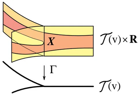
Fortunately, the following simple construction ([K4], Lemma 3.4), shown in Fig.3, produces an explicit recipe for recovering the triple $(X,\mathcal{F}(v),f)$ from the triple $({\partial }_{1}X,C_v,f^{\partial })$ but only up to a homeomorphism.

As we have seen in the proof of Theorem 2.1, the causality map $C_v$ determines the quotient trajectory space $\mathcal{T}(v)$ canonically. Let $f:X\to \mathbb{R}$ be a Lyapunov function for $v$.

The pair $(\mathcal{F}(v),f)$ gives rise to an embedding $\alpha :X\hookrightarrow \mathcal{T}(v)\times \mathbb{R}$, defined by the formula $\alpha (x)=([{\gamma }_x],f(x))$, where $x\in X$ and $[{\gamma }_x]\in \mathcal{T}(v)$ denotes the point-trajectory through $x$.

The dependence $x\to [{\gamma }_x]$ is continuous by the definition of the quotient topology in $\mathcal{T}(v)$.

Consider now the restriction ${\alpha }^{\partial }$ of the embedding $\alpha$ to the boundary ${\partial }_{1}X$. Evidently, the image of ${\alpha }^{\partial }:{\partial }_{1}X\hookrightarrow \mathcal{T}(v)\times \mathbb{R}$ bounds the image $\alpha (X)=\coprod _{[\gamma ]\in \mathcal{T}(v)}[f^{\partial }(\gamma \cap {\partial }_{1}X)]$. Therefore, using the product structure in $\mathcal{T}(v)\times \mathbb{R}$, ${\alpha }^{\partial }({\partial }_{1}X)$ determines $\alpha (X)$ canonically. Hence, $\alpha (X)$ depends on $C_v$ and $f_1^{\partial }$ only! Note that $\alpha$ is a continuous 1-to-1 map on a compact space, and thus, a homeomorphism onto its image. Moreover, the topological type of $X$ depends only on $C_v$: the apparent dependence of $\alpha (X)$ on $f^{\partial }$ is not crucial, since, for a given $v$, the space Lyapov(v) of Lyapunov functions for $v$ is convex.

The standing issue is: How to make sense of the claim " $\alpha$ is a diffeomorphism"? Section 3 describes our attempt to address this question (see Lemma 3.3 and Theorem 3.1).

III. RECOVERING THE ALGEBRA $C^{\mathrm{\infty }}(X)$ IN TERMS OF SUBALGEBRAS OF $C^{\mathrm{\infty }}({\partial }_{1}X)$

In what follows, we are inspired by the following classical property of functional algebras: for any compact smooth manifolds $X,Y$, we have an algebra isomorphism $C^{\mathrm{\infty }}(X\times Y)\approx C^{\mathrm{\infty }}(X)\hat{\otimes }{C}^{\mathrm{\infty }}(Y)$, where $\hat{\otimes }$ denotes an appropriate completion of the algebraic tensor product $C^{\mathrm{\infty }}(X)\otimes C^{\mathrm{\infty }}(Y)$ [Grot].

The trajectory space $\mathcal{T}(v)$, although a singular space, carries a surrogate smooth structure [K3]. By definition, a function $h:\mathcal{T}(v)\to \mathbb{R}$ is smooth if its pull-back ${\mathrm{\Gamma }}^{\ast }(h):X\to \mathbb{R}$ is a smooth function on $X$. As a subspace of $C^{\mathrm{\infty }}(X)$, the $C^{\mathrm{\infty }}(\mathcal{T}(v))$ is formed exactly by the smooth functions $g:X\to \mathbb{R}$, whose directional derivatives ${\mathcal{L}}_{v}g$ vanish in $X$. If ${\mathcal{L}}_v(g)=0$ and ${\mathcal{L}}_v(h)=0$, then ${\mathcal{L}}_v(g\cdot h)={\mathcal{L}}_v(g)\cdot h+g\cdot {\mathcal{L}}_v(h)=0$. Thus, $C^{\mathrm{\infty }}(\mathcal{T}(v))$ is indeed a subalgebra of $C^{\mathrm{\infty }}(X)$.

Note that if we change $v$ by a non-vanishing conformal factor $\lambda$, then ${\mathcal{L}}_{v}g=0$ if and only if ${\mathcal{L}}_{\lambda \cdot v}g=0$. Therefore, the algebra $C^{\mathrm{\infty }}(\mathcal{T}(v))$ depends only on the conformal class of $v$; in other words, on the foliation $\mathcal{F}(v)$.

In the same spirit, we may talk about diffeomorphisms ${\mathrm{\Phi }}^{\mathcal{T}}:\mathcal{T}(v)\to \mathcal{T}(v)$ of the trajectory spaces, as maps that induce isomorphisms of the algebra $C^{\mathrm{\infty }}(\mathcal{T}(v))$.

If two $(v$ -invariant) functions from $C^{\mathrm{\infty }}(\mathcal{T}(v))$ take different values at a point $[\gamma ]\in \mathcal{T}(v)$, then they must take different values on the finite set $\gamma \cap {\partial }_{1}X\subset {\partial }_{1}X$. Therefore, the obvious restriction homomorphism $re{s}_{\mathcal{T}}^{\partial }:C^{\mathrm{\infty }}(\mathcal{T}(v))\to C^{\mathrm{\infty }}({\partial }_{1}X)$, induced by the inclusion ${\partial }_{1}X\subset X$, is a monomorphism. We denote its image by $C^{\mathrm{\infty }}({\partial }_{1}X,v)$. Thus, we get an isomorphism $re{s}_{\mathcal{T}}^{\partial }:C^{\mathrm{\infty }}(\mathcal{T}(v))\to C^{\mathrm{\infty }}({\partial }_{1}X,v)$. We think of the subalgebra $C^{\mathrm{\infty }}({\partial }_{1}X,v)\subset C^{\mathrm{\infty }}({\partial }_{1}X)$ as an integral part of the boundary data for the holography problems we are tackling.

Let \pi_k: J^k(X,$\mathbb{R}$) \to X be the vector bundle of ,k,-jets of smooth maps from ,X, to ,$\mathbb{R}$,. We choose a continuous family semi-norms ,|\sim|_k, in the fibers of the jet bundle ,\pi_k, and use it to define a sup-norm ,|\sim|k, for the sections of ,\pi_k,. We denote by ,jet^k, the obvious map ,C^\infty(X,$\mathbb{R}$) \to J^k(X,$\mathbb{R}$), that takes each function ,h, to the collection of its ,k,-jets ,{jet_x^k(h)}{x\in X},.

The Whitney topology [W3] in the space $C^{\mathrm{\infty }}(X)=\{h:X\to \mathbb{R}\}$ is defined in terms of the countable family of the norms $\{\Vert je{t}^k(h){\Vert }_k{\}}_{k\in \mathbb{N}}$ of such sections $je{t}^k(h)$ of ${\pi }_k$. This topology insures the uniform convergence, on the compact subsets of $X$, of functions and their partial derivatives of an arbitrary order. Note also that $\Vert je{t}^k(h_1\cdot h_2){\Vert }_k\le \Vert je{t}^k(h_1){\Vert }_k\cdot \Vert je{t}^k(h_2){\Vert }_k$ for any $h_1,h_2\in C^{\mathrm{\infty }}(X)$.

Any subalgebra $\mathcal{A}\subset C^{\mathrm{\infty }}(X)$ inherits a topology from the Whitney topology in $C^{\mathrm{\infty }}(X)$. In particular, the subalgebra $C^{\mathrm{\infty }}(\mathcal{T}(v))\approx C^{\mathrm{\infty }}(X,v)$ does.

As a locally convex vector spaces, $C^{\mathrm{\infty }}(\mathcal{T}(v))$ and $C^{\mathrm{\infty }}(\mathbb{R})$ are then nuclear ([DS], [Ga]) so that the topological tensor product $C^{\mathrm{\infty }}(\mathcal{T}(v))\hat{\otimes }{C}^{\mathrm{\infty }}(\mathbb{R})$ (over $\mathbb{R}$ ) is uniquely defined as the completion of the algebraic tensor product $C^{\mathrm{\infty }}(\mathcal{T}(v))\otimes C^{\mathrm{\infty }}(\mathbb{R})$ [Grot].

We interpret $C^{\mathrm{\infty }}(\mathcal{T}(v))\hat{\otimes }{C}^{\mathrm{\infty }}(\mathbb{R})$ as the algebra of "smooth" functions on the product $\mathcal{T}(v)\times \mathbb{R}$ and denote it by $C^{\mathrm{\infty }}(\mathcal{T}(v)\times \mathbb{R})$.

Lemma 3.1. The intersection $C^{\mathrm{\infty }}(\mathcal{T}(v))\cap (f{)}^{\ast }(C^{\mathrm{\infty }}(\mathbb{R}))=\underset{―}{\mathbb{R}}$, the space of constant functions on $X$.

Proof. If a smooth function $h:X\to \mathbb{R}$ is constant on each $v$ -trajectory $\gamma$ and belongs to $(f{)}^{\ast }(C^{\mathrm{\infty }}(\mathbb{R}))$, then it must be constant on each connected leaf of $\mathcal{G}(f)$ that intersects $\gamma$. Thus, such $h$ is constant on the maximal closed connected subset $A_{\gamma }\subseteq f^{-1}(f(\gamma ))$ that contains $\gamma$. Each trajectory $\gamma$, homeomorphic to a closed interval, has an open neighborhood such that, for any trajectory ${\gamma }^{\prime }$ from that neighborhood, we have $A_{\gamma }\cap A_{{\gamma }^{\prime }}\ne \mathrm{\varnothing }$. Since $X$ is connected, any pair $\gamma ,{\gamma }^{\prime }$ of trajectories may be connected by a path $\delta \subset X$. Using the compactness of $\delta$, we conclude that the function $h$ must be a constant along $\delta$. Therefore, $h$ is a constant globally.

Let us consider two subalgebras, $f^{\ast }(C^{\mathrm{\infty }}(\mathbb{R}))\subset C^{\mathrm{\infty }}(X)$ and $(f^{\partial }{)}^{\ast }(C^{\mathrm{\infty }}(\mathbb{R}))\subset C^{\mathrm{\infty }}({\partial }_{1}X)$, the second one is assumed to be a "known" part of the boundary data.

Lemma 3.2. The restriction operator $H_f^{\partial }:f^{\ast }(C^{\mathrm{\infty }}(\mathbb{R}))\to (f^{\partial }{)}^{\ast }(C^{\mathrm{\infty }}(\mathbb{R}))$ to the boundary ${\partial }_{1}X$ is an epimorphism of algebras. If the range $f^{\partial }({\partial }_{1}X)$ of $f^{\partial }$ is a connected closed interval of $\mathbb{R}$ (which is the case for a connected ${\partial }_{1}X$ ), then $H_f^{\partial }$ is an isomorphism.

Proof. The restriction operator $H_f^{\partial }$ is an algebra epimorphism, since any composite function $\varphi \circ f^{\partial }$, where $\varphi \in C^{\mathrm{\infty }}(\mathbb{R})$, is the restriction to ${\partial }_{1}X$ of the function $\varphi \circ f$.

On the other hand, when $f^{\partial }({\partial }_{1}X)$ is a connected subset of $\mathbb{R}$, we claim that $H_f^{\partial }$ is a monomorphism. Indeed, take a function $\varphi \in C^{\mathrm{\infty }}(\mathbb{R})$, such that $\varphi \circ f^{\partial }\equiv 0$, but $\varphi \circ f$ is not identically zero on $X$. Then there is $x\in X$ such that $\varphi \circ f(x)\ne 0$. On the other hand, by the hypothesis, $f(x)=f^{\partial }(y)$ for some $y\in {\partial }_{1}X$. By the assumption, $f^{\partial }\circ \varphi \equiv 0$ which implies that $\varphi (f^{\partial }(y))=0$. This contradiction validates the claim about $H_f^{\partial }$ being a monomorphism. Therefore, when $f^{\partial }({\partial }_{1}X)$ is a connected interval, $H_f^{\partial }$ is an isomorphism of algebras.

Consider the homomorphism of algebras

that takes every finite sum $\sum _i{h}_i\otimes (f\circ g_i)$, where $h_i\in C^{\mathrm{\infty }}(\mathcal{T}(v))\subset C^{\mathrm{\infty }}(X)$ and $g_i\in C^{\mathrm{\infty }}(\mathbb{R})$, to the finite sum $\sum _i{h}_i\cdot (g_i\circ f)\in C^{\mathrm{\infty }}(X)$.

Recall that, by Lemma 3.1, $C^{\mathrm{\infty }}(\mathcal{T}(v))\cap (f{)}^{\ast }(C^{\mathrm{\infty }}(\mathbb{R}))=\underset{―}{\mathbb{R}}$, the constants. For any linearly independent $\{h_i{\}}_i$, this lemma implies that if $\sum _i{h}_i\cdot (g_i\circ f)\equiv 0$, then $\{g_i\circ f\equiv 0{\}}_i$; therefore, $\mathsf{P}$ is a monomorphism.

Let us compare the, so called, projective crossnorms {| \sim |k}{k \in $\mathbb{Z}$_+} (see (3.1)) of an element

and the norms of the element $\mathsf{P}(\varphi )=\sum _i{h}_i\cdot (f\circ g_i)$. By comparing the Taylor polynomial of the product of two smooth functions with the product of their Taylor polynomials, we get that, for all $k\in {\mathbb{Z}}_{+}$,

where inf is taken over all the representations of the element $\varphi \in C^{\mathrm{\infty }}(\mathcal{T}(v))\otimes f^{\ast }(C^{\mathrm{\infty }}(\mathbb{R}))$ as a sum $\sum _i{h}_i\otimes (f\circ g_i)$. Here we may assume that all $\{h_i{\}}_i$ are linearly independent elements and so are all $\{f\circ g_i{\}}_i$; otherwise, a simpler representation of $\varphi$ is available.

By the inequality in (3.1), $\mathsf{P}$ is a bounded (continuous) operator. As a result, by continuity, $\mathsf{P}$ extends to an algebra homomorphism

whose source is the completion of the algebraic tensor product $C^{\mathrm{\infty }}(\mathcal{T}(v))\otimes f^{\ast }(C^{\mathrm{\infty }}(\mathbb{R}))$

Lemma 3.3. The embedding $\alpha :X\to \mathcal{T}(v)\times \mathbb{R}$ (introduced in the end of Section 2 and depicted in Fig. 3) induces an algebra epimorphism

Moreover, the map $\hat{\mathsf{P}}$ is an isomorphism.

Proof. First, we claim that the subalgebra $\mathsf{P}(C^{\mathrm{\infty }}(\mathcal{T}(v))\otimes f^{\ast }(C^{\mathrm{\infty }}(\mathbb{R})))\subset C^{\mathrm{\infty }}(X)$ satisfies the three hypotheses of Nachbin's Theorem [Na]. Therefore, by [Na], the $\mathsf{P}$ -image of $C^{\mathrm{\infty }}(\mathcal{T}(v))\otimes f^{\ast }(C^{\mathrm{\infty }}(\mathbb{R}))$ is dense in $C^{\mathrm{\infty }}(X)$. Let us validate these three hypotheses.

(1) For each $x\in X$, there is a function $q\in C^{\mathrm{\infty }}(\mathcal{T}(v))\otimes f^{\ast }(C^{\mathrm{\infty }}(\mathbb{R}))$ such that $q(x)\ne 0$. Just take $q=f\circ (t+c)$, where and $t:\mathbb{R}\to \mathbb{R}$ is the identity. (2) For each $x,y\in X$, there is a function $q\in C^{\mathrm{\infty }}(\mathcal{T}(v))\otimes f^{\ast }(C^{\mathrm{\infty }}(\mathbb{R}))$ such that $q(x)\ne q(y)$ (i.e., the algebra $C^{\mathrm{\infty }}(\mathcal{T}(v))\otimes f^{\ast }(C^{\mathrm{\infty }}(\mathbb{R}))$ separates the points of $X$ ). If $f(x)\ne f(y)$, $q=f$ will do. If $f(x)=f(y)$, but $[{\gamma }_x]\ne [{\gamma }_y]$, then there is a $v$ -invariant function $h\in C^{\mathrm{\infty }}(\mathcal{T}(v))$ such that $h(x)=1$ and $h(y)=0$. To construct this $h$, we take a transversal section $S_x\subset \hat{X}$ of the $\hat{v}$ -flow in the vicinity of $x$ such that all the $\hat{v}$ -trajectories through $S_x$ are distinct from the trajectory ${\gamma }_y$. We pick a smooth function $\tilde{h}:S_x\to \mathbb{R}$ such that $h$ is supported in $\mathrm{int}(S_x)$, vanishes with all its derivatives along the boundary $\partial S_x$, and $\tilde{h}(x)=1$. Let $\mathcal{S}$ denote the set of $\hat{v}$ -trajectories through $S_x$. Of course, $\tilde{h}$ extends to a smooth function $h^{†}:\mathcal{S}\to \mathbb{R}$ so that $h^{†}$ is constant along each trajectory from $\mathcal{S}$. We denote by $h^{‡}$ the obvious extension of $h^{†}$ by the zero function. Finally, the restriction $h$ of $h^{‡}$ to $X$ separates $x$ and $y$. (3) For each $x\in X$ and $w\in T_{x}X$, there is a function $q\in C^{\mathrm{\infty }}(\mathcal{T}(v))\otimes f^{\ast }(C^{\mathrm{\infty }}(\mathbb{R}))$ such that $d{q}_x(w)\ne 0$.

Let us decompose $w=av+b{w}^{†}$, where $a,b\in \mathbb{R}$ and the vector $w^{†}$ is tangent to the hypersurface $S_x={\hat{f}}^{-1}(f(x))$. Then, if $a\ne 0$, then $df(w)\ne 0$. If $a=0$, then the there is a function $\tilde{h}:S_x\to \mathbb{R}$ which, with all its derivatives, is compactly supported in the vicinity of $x$ in $S_x$ and such that $d{\tilde{h}}_x(w^{†})\ne 0$. As in the case (2), this function extends to a desired function $h\in C^{\mathrm{\infty }}(\mathcal{T}(v))$. Now put $q=h\otimes 1$.

As a result, the image of $\mathsf{P}:C^{\mathrm{\infty }}(\mathcal{T}(v))\otimes f^{\ast }(C^{\mathrm{\infty }}(\mathbb{R}))⟶C^{\mathrm{\infty }}(X)$ is dense. Therefore, $\hat{\mathsf{P}}$ and, thus, $(\alpha {)}^{\ast }:C^{\mathrm{\infty }}(\mathcal{T}(v))\hat{\otimes }{C}^{\mathrm{\infty }}(\mathbb{R})⟶C^{\mathrm{\infty }}(X)$ are epimorphisms.

Let us show that $\hat{\mathsf{P}}$ is also a monomorphism. Take a typical element

viewed as a sum that converges in all the norms | \sim |k from (3.1). We aim to prove that if \hat{\mathsf{P}}(\theta) = \sum{i=1}^\infty h_i \cdot (f \circ g_i) vanishes on X, then \theta = 0.

For each point $x\in \mathrm{int}(X)$, there is a small closed cylindrical solid $H_x\subset \mathrm{int}(X)$ that contains $x$ and consists of segments of trajectories through a small $n$ -ball $D^n\subset f^{-1}(f(x))$, transversal to the flow. Thus, the product structure $D^1\times D^n$ of the solid $H_x$ is given by the $v$ -flow and the Lyapunov function $f:X\to \mathbb{R}$.

We localize the problem to the cylinder $H_x$. Consider the commutative diagram

where $\mathbf{res}:C^{\mathrm{\infty }}(X)\to C^{\mathrm{\infty }}(H_x)$ is the natural homomorphism,

and $\hat{\mathbf{Q}}(\sum _{i=1}^{\mathrm{\infty }}{\tilde{h}}_i\otimes {\tilde{g}}_i){=}_{\mathtt{def}}\sum _{i=1}^{\mathrm{\infty }}{\tilde{h}}_i\cdot {\tilde{g}}_i$ for ${\tilde{h}}_i\in C^{\mathrm{\infty }}(D^n)$, ${\tilde{g}}_i\in C^{\mathrm{\infty }}(D^1)$.

Since \hat{\mathbf{Q}} is an isomorphism [Grot] and \hat{\mathrm{P}} (\theta) = 0, it follows from (3.5) that \theta \in \ker (\mathrm{res}^{\prime}$\hat{\otimes }$\mathrm{res}^{\prime\prime}) for any cylinder \mathit{H}x. After reshuffling terms in the sum, one may assume that all the functions {h_i|{D^n}}i are linearly independent. Using that the functions h_i|{D^n} and (f\circ g_i)|_{D^1} depend of the complementary groups of coordinates in \mathit{H}_x, we conclude that these functions must vanish for any \mathit{H}_x \subset $\mathrm{int}$(X). As a result, \theta = 0 globally in $\mathrm{int}$(X) and, by continuity, \theta vanishes on \mathit{X}.

Consider now the "known" homomorphism of algebras

utilizing the boundary data. Here, by the definition of $C^{\mathrm{\infty }}({\partial }_{1}X,v)$, ${\mathsf{res}}_{\mathcal{T}}^{\partial }:C^{\mathrm{\infty }}(\mathcal{T}(v))\to C^{\mathrm{\infty }}({\partial }_{1}X,v)$ is an isomorphism, and ${\hat{\mathsf{R}}}^{\partial }$ denotes the completion of the bounded homomorphism ${\mathsf{R}}^{\partial }$ that takes each element $\sum _i{h}_i\otimes (f^{\partial }\circ g_i)$, where $h_i\in C^{\mathrm{\infty }}({\partial }_{1}X,v)$ and $g_i\in C^{\mathrm{\infty }}(\mathbb{R})$ to the sum $\sum _i{h}_i\cdot (g_i\circ f^{\partial })$.

The next lemma shows that the hypotheses of Theorem 3.1 are not restrictive, even when ${\partial }_{1}X$ has many connected components.

Lemma 3.4. Any traversing vector field $v$ on a connected compact manifold $X$ admits a Lyapunov function $f:X\to \mathbb{R}$ such that $f(X)=f({\partial }_{1}X)$.

Proof. Note that, for any Lyapunov function $f$, the image $f({\partial }_{1}X)$ is a disjoint union of finitely many closed intervals $\{I_k=[a_k,b_k]{\}}_k$, where the index $k$ reflects the natural order of intervals in $\mathbb{R}$. We will show how to decrease, step by step, the number of these intervals by deforming the original function $f$. Note that the local extrema of any Lyapunov function on $X$ occur on its boundary ${\partial }_{1}X$ and away from the locus ${\partial }_{2}X(v)$ where $v$ is tangent to ${\partial }_{1}X$. Consider a pair of points $A_{k+1},B_k\in {\partial }_{1}X\setminus {\partial }_{2}X(v)$ such that $f(A_{k+1})=a_{k+1}$ and $f(B_k)=b_k$, where . Then we can increase $f$ in the vicinity of its local maximum $B_k$ so that the $B_k$ -localized deformation $\tilde{f}$ of $f$ has the property and $\tilde{f}$ is a Lyapunov function for $v$. This construction decreases the number of intervals in $\tilde{f}({\partial }_{1}X)$ in comparison to $f({\partial }_{1}X)$ at least by one.

We are ready to state the main result of this paper.

Theorem 3.1. Assuming that the range $f^{\partial }({\partial }_{1}X)$ is a connected interval of $\mathbb{R}$, the algebra $C^{\mathrm{\infty }}(X)$ is isomorphic to the subalgebra

Moreover, by combining (3.2) with (3.4), we get a commutative diagram

whose vertical homomorphism $\mathrm{id}\hat{\otimes }{H}_f^{\partial }$ and the horizontal homomorphism $\hat{\mathsf{R}}$ are isomorphisms, and the vertical epimorphism $\mathrm{res}$ is the obvious restriction operator.

As a result, inverting $\mathbf{id}\hat{\otimes }{H}_f^{\partial }$, we get an algebra isomorphism

Proof. Consider the commutative diagram (3.5). Its upper-right conner is "unknown", while the lower row is "known" and represents the boundary data, and res is obviously an epimorphism. By Lemma 3.2, the left vertical arrow $\mathrm{id}\hat{\otimes }{H}_f^{\partial }$ is an isomorphism. Since, by Lemma 3.3, $\hat{\mathsf{R}}$ is an isomorphism, it follows that $\hat{\mathsf{R}}\circ (\mathrm{id}\hat{\otimes }{H}_f^{\partial }{)}^{-1}$ must be an isomorphism as well. In particular, ${\hat{\mathsf{R}}}^{\partial }$ is an epimorphism, whose kernel is isomorphic to the smooth functions on $X$ whose restrictions to ${\partial }_{1}X$ vanish. If $z\in C^{\mathrm{\infty }}(X)$ is a smooth function such that zero is its regular value, $z^{-1}(0)={\partial }_{1}X$, and in $\mathrm{int}(X)$, then the kernel of res is the principle ideal $\mathfrak{m}(z)$, generated by $z$. Therefore, by the commutativity of (3.5), the kernel of the homomorphism ${\hat{\mathsf{R}}}^{\partial }$ must be also a principle ideal ${\mathfrak{M}}_{\partial }$, generated by an element $(\hat{\mathsf{R}}\circ (\mathrm{id}\hat{\otimes }{H}_f^{\partial }){)}^{-1}(z)$.

Corollary 3.1. If the range $f^{\partial }({\partial }_{1}X)$ is a connected interval in $\mathbb{R}$, then the two topological algebras $C^{\mathrm{\infty }}({\partial }_{1}X,v)\subset C^{\mathrm{\infty }}({\partial }_{1}X)$ and $(f^{\partial }{)}^{\ast }(C^{\mathrm{\infty }}(\mathbb{R}))\subset C^{\mathrm{\infty }}({\partial }_{1}X)$ determine, up to an isomorphism, the algebra $C^{\mathrm{\infty }}(X)$, and thus determine the smooth topological type of the manifold $X$.

Proof. We call a maximal ideal of an algebra $\mathcal{A}$ nontrivial if it is different from $\mathcal{A}$.

By Theorem 3.1, the algebra $C^{\mathrm{\infty }}(X)$ is determined by the two algebras on ${\partial }_{1}X$, up to an isomorphism. In turn, the algebra $C^{\mathrm{\infty }}(X)$ determines the smooth topological type of $X$, viewed as a ringed space. This fact is based on interpreting $X$ as the space $\mathcal{M}(C^{\mathrm{\infty }}(X))$ of nontrivial maximal ideals of the algebra $C^{\mathrm{\infty }}(X)$ [KMS].

Let ${\mathfrak{m}}_v^{\partial }◃C^{\mathrm{\infty }}({\partial }_{1}X,v)$ and ${\mathfrak{m}}_f^{\partial }◃(f^{\partial }{)}^{\ast }(C^{\mathrm{\infty }}(\mathbb{R}))$ be a pair of nontrivial maximal ideals. Note that ${\mathfrak{m}}_v^{\partial }={\mathfrak{m}}_v^{\partial }([\gamma ])$ consists of functions from $C^{\mathrm{\infty }}({\partial }_{1}X,v)$ that vanish on the locus $\gamma \cap {\partial }_{1}X$, and ${\mathfrak{m}}_f^{\partial }={\mathfrak{m}}_f^{\partial }(c)$ consists of functions from $(f^{\partial }{)}^{\ast }(C^{\mathrm{\infty }}(\mathbb{R}))$ that vanish on the locus ${\partial }_{1}X\cap f^{-1}(c)$, where $c\in f({\partial }_{1}X)\subset \mathbb{R}$. We denote by $⟨{\mathfrak{m}}_v^{\partial },{\mathfrak{m}}_f^{\partial }⟩$ the maximal ideal of $C^{\mathrm{\infty }}({\partial }_{1}X,v)\hat{\otimes }(f^{\partial }{)}^{\ast }(C^{\mathrm{\infty }}(\mathbb{R}))$ that contains both ideals ${\mathfrak{m}}_v^{\partial }\hat{\otimes }1$ and $1\hat{\otimes }{\mathfrak{m}}_f^{\partial }$. If the range $f^{\partial }({\partial }_{1}X)$ is a connected interval of $\mathbb{R}$ and $⟨{\mathfrak{m}}_v^{\partial },{\mathfrak{m}}_f^{\partial }⟩$ is a nontrivial ideal, then $\gamma \cap f^{-1}(c)\ne \mathrm{\varnothing }$. Otherwise, $\gamma \cap f^{-1}(c)=\mathrm{\varnothing }$. Therefore, with the help of the isomorphism $\mathcal{H}(v,f)$ from (3.6), the nontrivial maximal ideals of $C^{\mathrm{\infty }}(X)$ (which by [KMS] correspond to points $x=\gamma \cap f^{-1}(c)\in X$ ) are of the form $\mathcal{H}(v,f)(⟨{\mathfrak{m}}_v^{\partial },{\mathfrak{m}}_f^{\partial }⟩)$.

Corollary 3.2. Let the range $f^{\partial }({\partial }_{1}X)$ be a connected interval of $\mathbb{R}$. With the isomorphism $\mathcal{H}(v,f)$ from (3.6) being fixed, any algebra isomorphism ${\mathrm{\Psi }}^{\partial }:C^{\mathrm{\infty }}({\partial }_{1}X)\to C^{\mathrm{\infty }}({\partial }_{1}X)$ that preserves the subalgebras $C^{\mathrm{\infty }}({\partial }_{1}X,v)$ and $(f^{\partial }{)}^{\ast }(C^{\mathrm{\infty }}(\mathbb{R}))$ extends canonically to the algebra isomorphism $\mathrm{\Psi }:C^{\mathrm{\infty }}(X)\to C^{\mathrm{\infty }}(X)$.

Thus, an action of any group $\mathsf{G}$ of such isomorphisms ${\mathrm{\Psi }}^{\partial }$ extends canonically to a $\mathsf{G}$ -action on the algebra $C^{\mathrm{\infty }}(X)$ and, via it, to a $\mathsf{G}$ -action on $X$ by smooth diffeomorphisms.

Proof. By [Mr], any algebra isomorphism $\mathrm{\Psi }:C^{\mathrm{\infty }}(X_1)\to C^{\mathrm{\infty }}(X_2)$ is induced by a unique smooth diffeomorphism $\mathrm{\Phi }:X_1\to X_2$. With this fact in hand, by Theorem 2.1 and Theorem 3.1, the proof is on the level of definitions.

It remains to address the following crucial question: how to characterize intrinsically the trace $C^{\mathrm{\infty }}({\partial }_{1}X,v)$ of the algebra $C^{\mathrm{\infty }}(\mathcal{T}(v))\approx \ker \{{\mathcal{L}}_v:C^{\mathrm{\infty }}(X)\to C^{\mathrm{\infty }}(X)\}$ in the algebra $C^{\mathrm{\infty }}({\partial }_{1}X)$?

Evidently, functions from $C^{\mathrm{\infty }}({\partial }_{1}X,v)$ are constant along each $C_v$ -"trajectory" ${\gamma }^{\partial }:=\gamma \cap {\partial }_{1}X$ of the causality map. Furthermore, any smooth function $\psi :{\partial }_{1}X\to \mathbb{R}$ that is constant on each finite set ${\gamma }^{\partial }$ gives rise to a unique continuous function $\varphi$ on $X$ that is constant along each $v$ -trajectory $\gamma$. However, such functions $\varphi$ may not be automatically smooth on $X$ (a priori, they are just Hölderian with some control of the Hölder exponent that depends on the dimension of $X$ only)! This potential complication leads to the following question.

Question 3.1. For a traversing and boundary generic (alternatively, traversally generic) vector field $v$ on $X$, is it possible to characterize the subalgebra $C^{\mathrm{\infty }}({\partial }_{1}X,v)\subset C^{\mathrm{\infty }}({\partial }_{1}X)$ in terms of the causality map $C_v$ and, perhaps, some additional $v$ -generated data, residing in ${\partial }_{1}X$?

To get some feel for a possible answer, we need the notion of the Morse stratification of the boundary ${\partial }_{1}X$ that a vector field $v$ generates [Mo].

Let $\dim (X)=n+1$ and $v$ be a boundary generic traversing vector field on $X$.

Let us recall the definition of the Morse stratification $\{{\partial }_j^{\pm }X(v){\}}_{j\in [1,n+1]}$ of ${\partial }_{1}X$. We define the set ${\partial }_{2}X(v)$ as the locus where $v$ is tangent to ${\partial }_{1}X$. It separates ${\partial }_{1}X$ into ${\partial }_1^{+}X(v)$ and ${\partial }_1^{+}X(v)$. Let ${\partial }_{3}X(v)$ be the locus where $v$ is tangent to ${\partial }_{2}X(v)$. For a boundary generic $v$, ${\partial }_{2}X(v)$ is a smooth submanifold of ${\partial }_{1}X(v)$ and ${\partial }_{3}X(v)$ is a submanifold that divides ${\partial }_{2}X(v)$ into two regions, ${\partial }_2^{+}X(v)$ and ${\partial }_2^{-}X(v)$. Along ${\partial }_2^{+}X(v)$, $v$ points inside of ${\partial }_1^{+}X(v)$, and along ${\partial }_2^{-}X(v)$, $v$ points inside of ${\partial }_1^{-}X(v)$. This construction self-replicates until we reach finite sets ${\partial }_{n+1}^{\pm }X(v)$.

By definition, the boundary generic vector fields [K1] are the ones that satisfy certain nested transversality of $v$ with respect to the boundary ${\partial }_{1}X$, the transversality that guarantees that all the Morse strata ${\partial }_{j}X(v)$ are regular closed submanifolds and all the strata ${\partial }_j^{\pm }X(v)$ are compact submanifolds.

For a traversing boundary generic $v$, the map $C_v:{\partial }_1^{+}X(v)\to {\partial }_1^{-}X(v)$ makes it possible to recover the Morse stratification ([K4]).

Let us describe now a good candidate for the subalgebra $C^{\mathrm{\infty }}({\partial }_{1}X,v)$ in the algebra $C^{\mathrm{\infty }}(\partial X)$.

We denote by $\mathcal{L}$_v^{(k)} the k-th iteration of the Lie derivative $\mathcal{L}$v. Let $\mathsf{M}$(v) be the subalgebra of smooth functions \psi \colon ${\partial }_1$X \to $\mathbb{R}$ such that ($\mathcal{L}$v^{(k)}\psi)|{\partial{k+1}X(v)} = 0 for all k \leq n (by the Leibniz rule, $\mathsf{M}$(v) is indeed a subalgebra). Let us denote by $\mathsf{M}$(v)^{C_v} the subalgebra of functions from $\mathsf{M}$(v) that are constant on each (finite) C_v-trajectory \gamma^\partial \coloneqq \gamma \cap ${\partial }_1$X \subset ${\partial }_1$X.

Conjecture 3.1. Let $v$ be a traversing and boundary generic vector field on a smooth compact $(n+1)$ -manifold $X$. Then the algebra $C^{\mathrm{\infty }}({\partial }_{1}X,v)$ coincides with the subalgebra $\mathsf{M}(v{)}^{C_v}\subset C^{\mathrm{\infty }}({\partial }_{1}X)$.

In particular, $C^{\mathrm{\infty }}({\partial }_{1}X,v)$ can be determined by the causality map $C_v$ and the restriction of $v$ to ${\partial }_{2}X(v)$.

It is easy to check that $C^{\mathrm{\infty }}({\partial }_{1}X,v)\subset \mathsf{M}(v{)}^{C_v}$; the challenge is to show that the two algebras coincide.

The Holography Theorem (Corollary 2.1) has been established assuming Property A from Definition 2.1. If one assumes the validity of Conjecture 3.1, then, by Corollary 3.1, we may drop Property A from the hypotheses of the Holography Theorem. Indeed, the subalgebras $C^{\mathrm{\infty }}({\partial }_{1}X,v)$ and $(f^{\partial }{)}^{\ast }(C^{\mathrm{\infty }}(\mathbb{R})$ would acquire a description in terms of $C_v$ and $f^{\partial }$. This would deliver an independent proof of a natural generalization of Corollary 2.1.