I. INTRODUCTION

Savings is considered as one of the influencing element for economic growth of a country. Savings increase capital formation, and capital formation is an important factor for promoting economic development. According to Harrod (1939) and Domar (1946), savings leads to investment, and it leads to capital formation, which generates economic growth. It is improving efficiency of loanable funds and promoting capital accumulation (Shaw, 1973). Sustained accumulation of capital foster the economy to achieve higher and sustainable economic growth (Chow, 1993). In the short run, saving rate determine the speed of capital accumulation and growth in the economy (Ramsey, 1928). Savings increase capital formation and investment and thereby raising the growth of the economy (Abu, 2010).

Interest may function as an incentive to postpone gratification (Case, Fair, and Oster, 2012). In other words, it is the reward for postponing current consumption. Hence changes in interest rate may impact the savings such as lower interest rate is expected to stimulate current consumption and discourage savings and vice-versa. Aizenman et al. (2017) showed that the impact of the interest rate on saving is related to the capital accumulation which would determine future income level and thereby present-day consumption and saving in the long run. According to Case, Fair and, Oster (2012), "The final impact of a change in interest rates on saving depends on the relative size of the income and substitution effects." When the substitution effect crossed the income effect, saving tends to increase as the interest rate rises. Keynes argued that interest rate does not have a significant influence on the growth of savings in households and firms as retained profits and investment (Keynes, 1936). Some empirical studies indicated that interest rate could affect the savings positively (Shaw and McKinnon, 1973; Agrawal, 2007, Masson et al. 1998, Warman (1994) or negatively (Loayza et al., 2000). The people of an economy with aging population and insufficient social protection, may want to increase their savings for precautionary purposes if the interest rate is lower. According to Fry (1998), in an economy where interest rates are kept low, this leads to a decrease in current savings.

Bangladesh is an emerging economy that experienced on average more than 6 percent growth rate over the last decade. In FY 2020, during the pandemic situation, its growth rate was 5.2 percent. To expand its development, Bangladesh need to boost private investment. To increase private investment and create new jobs through industrialization Bangladesh decrease the deposit and lending rates by 6% and 9%, respectively. But the question is, what about the savings or deposit? The main objective of this paper is to know whether a lower interest rate has any impact on the saving of the Bangladesh economy?

a) Purpose of the study

The objective of this study is to investigate the impact of interest rate on gross saving in Bangladesh.

II. LITERATURE REVIEW

a) Theoretical Literature

The main theories on the saving behavior are: The Relative Income Hypothesis by Duesenberry (1949), the Permanent Income Hypothesis by Friedman (1957), the Life Cycle Hypothesis by Ando and Modigliani (1963), the Buffer-Stock Theory and The bequest theory. The life-cycle hypothesis developed by Modigliani and Brumberg (1954) predicted that individual consumption decisions depend on the lifetime expected income and saving patterns. This hypothesis assumes that individuals save to smooth their lifetime consumption. Thus individuals in their lifetime first act as a dissaver when they are child, savers while working and again dissolve when they retire.

The relative income hypothesis by Dusenberry (1949) states that the utility (satisfaction) derives from a given current consumption level is mainly depends on the status in the society rather than from the absolute level of income. Here consumer utility index depends on the ratio of consumption to a weighted average of the consumption of the other consumers. This hypothesis drew two conclusions: aggregate saving rate is independent of aggregate income, and the propensity to save of an individual is an increasing function of his or her percentile position in the income distribution.

The permanent income hypothesis formulated by Milton Friedman in 1957 implies that consumption behavior responds primarily to permanent income. That is, consumers do not respond equally to all income shocks. People will spend money at a level consistent with them appears permanent income. A worker will save only if the change in income is transitory or higher than the anticipated level of permanent income.

The Buffer-Stock Theory (Carrol, 1997) suggested that individuals set aside some precautionary reserve to avoid the unpredictable situation associated with future income fluctuation and smooth out future consumption levels. It assumes that consumers are impatient and prudent in the face of unpredictable income fluctuations.

b) Empirical Literature

Several empirical studies were conducted to find the relationship between interest rate and saving in different countries, but Bangladesh's perspective I could not find any significant studies regarding this topic. There are different views regarding this relationship. Some authors found that the interest rate effect savings negatively (Athukorala and Long Pang, 2003,) and some revealed a positive relationship between these variables (Khan et al., 1994, Sarantis and Stewart, 2001, Richard and Kolluri, 2003).

Joshua, et al. (2019) studied the interest rate effect on private saving by using the data of 135 countries from 1995 to 2014. They show that, a low interest rate can yield different effects on private saving under the different economic situations. If output volatility, old-age dependency, or financial development is above a certain threshold, the real interest rate affects the private saving negatively.

Ojeaga et al. (2014), examined the effect of interest rates on customer savings behavior in the Nigerian banking sector, and revealed that interest rates were probably increasing bank deposits.

Athukorala and Tsai (2003) investigated the determinants of household saving in Taiwan: Growth, demography, and public policy. They found that interest rate and savings positively related, whereas the relationship between inflation and saving is unfavorable.

Siaw and Lawer (2015) examined the determinants of bank deposits in long run and short run in Ghana by using a co-integration approach and revealed that, in the long-run, inflation and the deposit interest rate have a negative effect on bank deposit.

Mushtaq and Siddiqui (2017) investigated the effect of interest rates on bank deposits in Islamic and Non-Islamic economies for the period 1999 to 2014. By using the panel ARDL (Auto- regressive Distributed Lag) method, they revealed that there is no effect of interest rate on bank deposit in Islamic countries. In contrast, in Non- Islamic countries, interest rate and bank deposit are positively related.

Ang (2009) studied the determinants of household savings in India and China. The study results supported the life cycle model that growth in income and inflation stimulates the growth in household savings. In contrast age dependency has the opposite impact on savings. Furthermore, the results suggested that the expected increase in pension benefits tended to encourage savings in India in the long run, whereas the reverse association was found for China.

Loayza and Shankar (2000) examined the private savings trend in India by employing error correction model. They revealed that a significant positive association of per capita income, real interest rate, and agriculture share in GDP with private savings, whereas a significant negative association of financial development, inflation, and dependency ratio with the savings rate.

Murshed & Robin (2012) investigated the impact of the financial liberalization policy on the Bangladesh banking sector from 1981 to 2008. They found that insignificant positive association between domestic savings and the real interest rate.

Agrawal et al. 2007, studied saving behavior in South Asia. They concluded that the real interest rate positively affects the savings rate in Bangladesh and Nepal, whereas in India, Pakistan, and Sri Lanka, the effects are negative.

Masson et al. (1998) examined a broad set of possible determinants of private saving behavior by using sample data for industrial and developing countries. They obtained both time-series and cross-sectional estimates. The results suggest that demographics and growth are important determinants of private saving rates, and interest rates and terms of trade have positive but less robust effects.

Norman and Rashmi 2000, studied the private saving in India and found that real interest rate, Per capita income, and the share of agriculture in GDP has a positive effect on saving and financial development, inflation, and dependency ratio has a negative effect on saving in India.

Abduh et al. (2011) found that the interest rate and growth in production level do not significantly drive deposit.

Horioka (2009) investigated the saving behavior of the aged in Japan for 1990-2008. The author conducted the Family Income and Expenditure Survey to collect information on saving rates. The study found that dissaving had been made at retirement age, even working. The findings were consistent with the life cycle model.

Faridi et al. (2010) examined the determinants of household saving in the Multan district of Pakistan using the primary data. They concluded that spouse participation, total dependency rate, total income of household, and size of landholdings had a significant positive relationship with household saving. On the other hand, education household head, children's educational expenditures, family size, liabilities to be paid, marital status, and value of the house have a significant negatively relationship with household saving. This study supports the existence of the Life cycle hypothesis.

Wan et al. (2003) examined the determinants of rural China's savings behavior. The result revealed that undeveloped capital market structure and absence of social rights have a negative impact on rural savings behavior.

Aizenman, J. et al. 2017 investigated the interest rate effect on private saving: alternative perspectives using data on 135 countries from 1995 to 2014. The study showed that in an economy with a well-developed financial market, an aging population, and output volatility can all contribute towards turning the relationship between interest rates and saving negative. They detect the substitution effect of the real interest rate on private saving when the nominal interest rate is not too low among developing countries. The same results were detected among industrial and emerging economies only when the nominal interest rate is lower than 2.5%. In contrast, among emerging Asian countries, they found the income effect when the nominal interest rate is below 2.5%.

III. DATA

In this study, I used annual time-series data from the period 1976 to 2019. All data but remittance are collected from the world development indicators published by World Bank. The data of remittance is obtained from Bangladesh Bank.

IV. MODEL SPECIFICATION

The model of the study takes the form: Gross Saving as a function of Gross Domestic Product, Deposit Interest Rate, Remittance, and Inflation rate.

Here, ${\epsilon }_t$ is an error term which means there could be some other factors that can affect GS and ${\beta }_0$ is a scalar parameter, ${\beta }_1$, ${\beta }_2$, ${\beta }_3$, and ${\beta }_4$ are the slope coefficient parameters. All variables are transformed into log-linear form (LN). According to Shahbaz et al. (2013), modeling the log-log model specification will provide efficient results by mitigating the sharpness in time series data than the simple linear-linear specification.

Here, LNGS= log of Gross Saving that measured in percentage of GDP. LNINT= log of Deposit interest rate. LNINF= log of Inflation Rate, LNREM= log of remittance measured by million USD, LNGDP = log of real domestic savings. ${\beta }_0$ = the constant term ${\beta }_1$ = Coefficient of variable LNINT, ${\beta }_2$ = coefficient of variable LNINF, ${\beta }_3$ = coefficient of variable LNREM, ${\beta }_4$ = Coefficient of variable LNRGDP, t= the time trend. $\epsilon$ = the random error term Methodology.

I employ the Autoregressive Distributed Lag (ARDL) bound test to estimate the short run and long-run dynamic relationship among the selected variables for the study. This test recommended by Pesaran and Shin (1999) and Pesaran et al.2001. The advantages of the ARDL method it provides more robust result in a small sample size (30 to 80 observations); this approach is not sensitive to orders of integration of the variables of interest, It is applicable if some variables are I(0) and

(2) some are I(1); it is based on a single equation framework; the ARDL bound testing approach to co-integration yields efficient simultaneous estimation and separation of the short- and long-run relationships between the variables of interest; moreover the ARDL Approach yields unbiased estimates and valid - statistics, even if some of the regressors are endogenous (Paul et al.2011, Benzamin et al. 2001, and Narayan, 2005)

To employ this test, firstly we test the stationarity of the considered variables by using Augmented Dicked Fuller test (ADF) by Dickey and Fuller (1979, 1981) to see the order of integration. The ARDL is based on the assumption that the order of integrations of the variables are I(0)or I(1) (Ouattara, 2004). If any variables are integrated of I(2), the results can be spurious, and the ADRL bound test is unsuitable (Pesaran & Shin, 1998).

The equation for the ARDL test is as below:

Where $\mathrm{\Delta }$ represents the first differences of the variables, $\mathrm{\Sigma }$ 's represents the error correction dynamic, and $\beta$ 's shows the long-run relationship, ${\alpha }_0$ is the drift component and $\epsilon t$ is the white noise residuals. I analyzed the ARDL directly by using e-views 11. The null hypothesis that there is no co-integration among the variables against the alternative hypothesis of the existence of co-integration among the variables are given below:

The value of F-statistics is compared with the tabulated values of Narayan (2004) for the small sample size (30 to 80 observations). If the F-statistics value is greater than the upper critical value, reject the null hypothesis that means there exists a co-integration relationship or long-run relationship among the variables. If the value of F-statistics is less than the lower critical value, accept the null hypothesis, which means there is no co-integration among the variables. If, however, the F-statistics value lies within the upper and lower bound, the results are inconclusive. We employ the Akaike Information Criteria (AIC) to determine the optimal lag length for the study. The ARDL restricted ECM models is defined as:

Where $\psi$ is the speed of adjustment. ECM shows how much disequilibrium is being corrected (Emeka N., Kelvin U. (2016). A positive coefficient of ECM indicates a divergence, and a negative coefficient reveals a convergence. If the estimate of ECM = 1, 100% of the adjustment takes place each period that is the adjustment is instantaneous and full; if the estimate of ECM = 0.5, 50% of the adjustment is realized each period/year. ECM = 0 indicates that there is no adjustment, and no longer makes sense of the long-term relationship.

At last, to ensure the goodness of fit of the selected model author conduct the stability and diagnostic test. To check the stability of the parameters of the model, the author employs the stability test of the cumulative sum (CUSUM) of recursive residuals proposed by Pesaran and Pesaran (1997) and the cumulative sum of squares (CUSUMSQ) of recursive residuals by Brown et al. (1975).

V. RESULT

a) Unit Root Test

To check the stationary of the variables, researchers used the Augmented Dickey-Fuller (ADF) test. The result of the ADF test is given in table 1.

	ADF
Variable	At level		$1^{st}$ difference		Order of integration
	Constant	Constant, linear trend	Constant	Constant, linear trend
LNGS	-6.76***	-8.63***	--	--	I(0)
LNINT	-2.51	-3.53**	-4.41***	-4.54***	I(1)
LNINF	-5.87***	-5.69***	--	--	I(0)
LNREM	-4.92***	-2.72	-7.77***	-7.54***	I(1)
LNGDP	5.93	1.28	-4.51***	-7.63***	I(1)

Table 1 shows the test of stationary result. From the table, we can see that LNGS and LNINF are stationary at level, and LNINT, LNREM and LNGDP are nonstationary at level but stationary at 1st difference. Since some variables are integrated I(0) and some are I(1), we estimate ARDL long-run and short-run estimates.

b) Optimal Lag

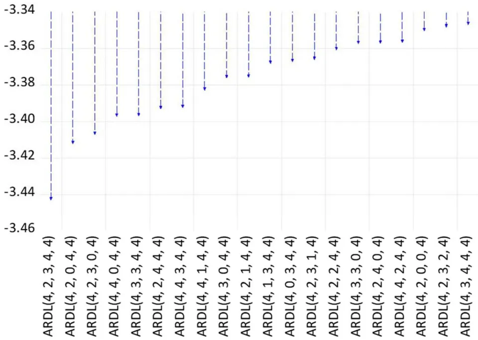
The result of the Akaike information criterion indicates that the optimal lag of the selected model is 4,2,3 4,4, shown in figure 1.

Akaike Information Criteria (top 20 models) Figure 1: Optimal Lag

c) Bound Test and Cointegration Result Table 2: Summery of Bound Test

Test Statistic	Value	Signif.	I(0)	I(0)
F-statistic	19.15076	10%	2.2	30.9
K	4	5%	2.56	3.49
		2.5%	2.88	3.87
		1%	3.29	4.37

Table 2 shows the result of the Bound F-test. The calculated F value for LNGS is 19.15076, which is higher than all the lower and upper bound limits at 1%, 2.25%, 5%, and 10%. So we can reject the null hypothesis of "no cointegration (long-run relation) between dependent and explanatory variables," that is there exists a long-run relationship between LNGS and all other independent variables used in this study.

d) Long-Run Estimates of ARDL Approach Table 3: Result of the Long-Run Estimates

Variable	Coefficient	Std. Error	t-Statistic	Prob.
C	-3.935830	2.103135	-1.871411	0.0776
LNGS(-1)*	-0.187539	0.147794	-1.268926	0.2206
LNINT(-1)	0.065857	0.080417	0.818947	0.4235
LNINF(-1)	0.047654	0.019725	2.415943	0.0265
LNGDP(-1)	0.527124	0.213428	2.469800	0.0238
LNREM(-1)	-0.205587	0.116166	-1.769775	0.0937
D(LNGS(-1))	-0.362844	0.105207	-3.448844	0.0029
D(LNGS(-2))	-0.371500	0.085932	-4.323164	0.0004
D(LNGS(-3))	-0.507882	0.054989	-9.236030	0.0000
D(LNINT)	-0.008119	0.082693	-0.098179	0.9229
D(LNINT(-1))	0.130041	0.084103	1.546216	0.1395
D(LNINF)	0.021211	0.011953	1.774513	0.0929
D(LNINF(-1))	-0.023879	0.014291	-1.670931	0.1120
D(LNINF(-2))	-0.018072	0.011329	-1.595234	0.1281
D(LNGDP)	1.236912	1.101880	1.122547	0.2764
D(LNGDP(-1))	0.663201	1.003260	0.661046	0.5170
D(LNGDP(-2))	-0.709099	1.048418	-0.676352	0.5074
D(LNGDP(-3))	-1.752997	0.901423	-1.944700	0.0676
D(LNREM)	0.157008	0.088557	1.772964	0.0932
D(LNREM(-1))	0.409585	0.117412	3.488436	0.0026
D(LNREM(-2))	0.504683	0.099336	5.080553	0.0001
D(LNREM(-3))	0.197701	0.066752	2.961736	0.0084

Table 3 shows the long-run coefficient of the ARDL model. The result indicates that the previous year's deposit interest rate (INT) has a positive impact on current year gross savings (GS) but not significant. This result is similar to Murshed & Robin (2012). Moreover, inflation and gross domestic product (GDP) bear a significant (at 5 percent) positive impact on gross savings. That is, if 1 percent increase in last year's inflation, gross savings will increase in approximately 5

e) Short-Run Analysis of ARDL

Variable	Coefficient	Std. Error	t-Statistic	Prob.
D(LNGS(-1))	-0.362844	0.053651	-6.763049	0.0000
D(LNGS(-2))	-0.371500	0.041358	-8.982546	0.0000
D(LNGS(-3))	-0.507882	0.030235	-16.79802	0.0000
D(LNINT)	-0.008119	0.056850	-0.142809	0.8880
D(LNINT(-1))	0.130041	0.054674	2.378472	0.0287
D(LNINF)	0.021211	0.008764	2.420268	0.0263
D(LNINF(-1))	-0.023879	0.008491	-2.812294	0.0115
D(LNINF(-2))	-0.018072	0.007541	-2.396547	0.0276
D(LNGDP)	1.236912	0.736604	1.679209	0.1104
D(LNGDP(-1))	0.663201	0.676282	0.980658	0.3398
D(LNGDP(-2))	-0.709099	0.726844	-0.975586	0.3422
D(LNGDP(-3))	-1.752997	0.664443	-2.638298	0.0167
D(LNREM)	0.157008	0.062506	2.511872	0.0218
D(LNREM(-1))	0.409585	0.054956	7.453029	0.0000
D(LNREM(-2))	0.504683	0.042967	11.74581	0.0000
D(LNREM(-3))	0.197701	0.044943	4.398973	0.0003
CointEq(-1)*	-0.187539	0.015477	-12.11703	0.0000
R-squared	0.977401	Mean dependent var		0.040433
Adjusted R-squared	0.961679	S.D. dependent var		0.168222
S.E. of regression	0.032931	Akaike info criterion		-3.692219
Sum squared resid	0.024942	Schwarz criterion		-2.974445
Log likelihood	90.84438	Hannan-Quinn criter.		-3.432695
Durbin-Watson stat	1.536555

Table 4 shows the short-run ARDL result summary that indicates in the short-run impact of interest rate on gross saving is negative but not statistically significant that is in the current year, increase in interest rate decrease the saving rate. The result also reveals that inflation and remittance have a positive with significant impact and GDP has an insignificant positive impact on gross savings in Bangladesh.

Estimated results also exhibit that the sign of the lagged error correction representations ( $EC{M}_{t-1}$ ) is negative and statistically significant at 5 percent indicates the speed of adjustment toward long-run equilibrium. The coefficient of -0.19, for instance, implies that approximately 19 percent disequilibrium from the previous year's shock converges on the long-run equilibrium in the current year. The result reveals that the $R^2$ value is 0.97, which reflects that 97 percent variation of the dependent variable explained by the independent variables. The value of adjusted $R^2$ is 96 percent. The Durbin-Watson (D-W) value is 1.536555, which confirms that no autocorrelation among the variables. The statistics' ( $R^2$, Adj. $R^2$; D-W) results show that our model is robust and well fitted.

f) Stability Test

To check the stability of the model, I used cusum and cusum square test. The result of the tests is given by following figure 2 and figure 3:

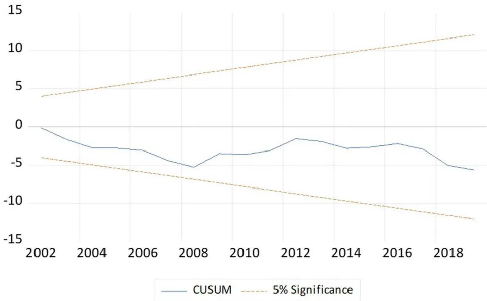
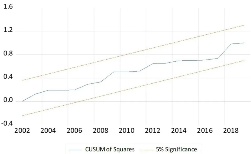
We can see above figures 2 and 3 that the CUSUM line and the CUSUM of Squares line lie between the critical bounds of 5 percent significant, which indicates the stability of all coefficients in the estimated model.

g) Diagnostic Test

A residual diagnostic test was applied for checking autocorrelation, heteroscedasticity, and serial correlation in the residual.

i. Test of Normality

To check whether the data used in the model are normally distributed or not, I employ the Jarque Bera test. Here the null and alternative hypothesis are:

Ho: The data are normally distributed, and

H1: The data are not normally distributed.

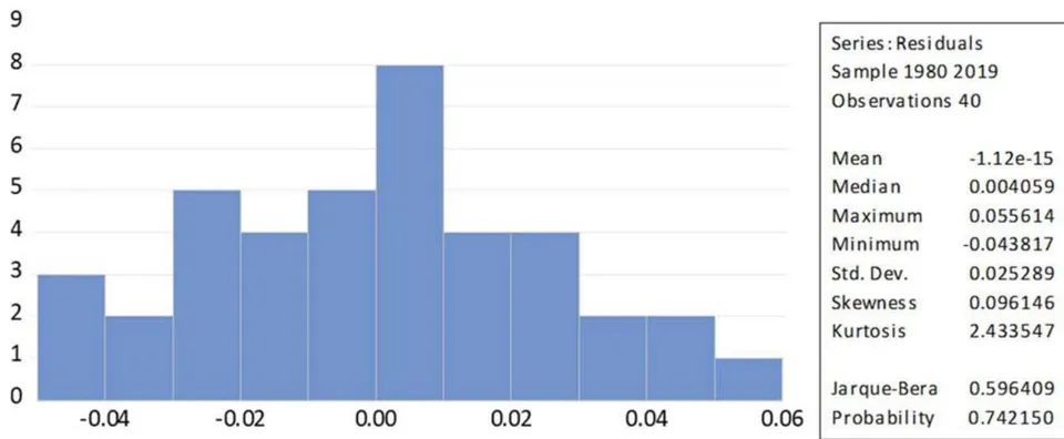
The result of the Jarque Bera test shows that the value of the test is 0.596409 and the corresponding p-value is 0.742150, which is greater than 0.05. that means we cannot reject the null hypothesis. Hence the estimated model is normally distributed.

hypothesis and alternative hypothesis are: Ho: there is no serial correlation in the residual. H1: there is a serial correlation in the residual.

ii. Test for Serial Correlation

The existence of serial correlation is tested by Breusch-Godfrey Serial Correlation LM Test. The null

F-statistic	0.687429	Prob. F(2,16)	0.5171
Obs*R-squared	3.165165	Prob. Chi-Square(2)	0.2054

From Table 5, we can see that the Obs* R squared is 3.16 and the p-value is 0.20. Here p-value > 0.05, hence we cannot reject the null hypothesis; instead, we reject the alternative hypothesis, which indicates that there is no serial correlation in the residual.

iii. Test for Heteroskedasticity

I used the Breusch-Pagan-Godfrey test to detect heteroscedasticity. Here we can take two hypotheses: Ho: Homoskedasticity H1: Heteroskedasticity.

F-statistic	0.711667	Prob. F(21,18)	0.7741
Obs*R-squared	18.14540	Prob. Chi-Square(21)	0.6398
Scaled explained SS	2.633745	Prob. Chi-Square(21)	1.0000

Table 6 shows the result summary of the Breusch-Pagan-Godfrey test. From the table, we can see that obs* r-squared p-value is 0.6398, which is greater than 0.05, so we can reject the alternative hypothesis and accept the null hypothesis. That is, there is no heteroskedasticity in this model.

VI. CONCLUSION

In this paper, I focused on whether the recent lower deposit interest rate will create any monetary uncertainty by discouraging people to save in Bangladesh. In this study, I used deposit interest rate, inflation rate, remittance, and GDP as explanatory variables. I used time-series data from the period of 1976 to 2019. In my current study, I employed the ARDL approach to investigate the long-run and short-run impact of selected variables on gross savings. The stationarity of all variables was check and we found that some variables were integrated at the first difference, and some were at the level. The Akaike information criterion was applied to get the optimal model, and the suggested optimal model was 4,2,3,4,4. The results of the study revealed in the short-run lower interest rate increase gross saving that indicates that people save their money for the precautionary purpose not for interest or profit but in the long-run relationship between deposit interest rate and gross saving is positive but insignificant that is higher interest lead to higher gross savings and lower interest rate lower the saving. In the long-run and short-run inflation and GDP have a positive influence on gross savings. Result also displayed that in the long-run previous year remittance discourage the current year savings, and in the short run it encourages saving behavior in Bangladesh. From this investigation, it can be said that in the long period, lower deposit interest rate may negatively effect capital formation by reducing savings.