## I. INTRODUCTION A structural discontinuity emerges whenever there is a sudden change in the cross-sectional shape of a structural section. This can occur in various scenarios, such as when there are openings in decks, hatches, and machinery, access points on sidewalls, cutouts in web plates, or holes in crankshafts, among other instances. These irregularities in the structure can alter how stress is distributed within it, leading to the introduction of stresses around the edges of holes or at the ends of cracks. Professionals from various fields, including hydrodynamic experts, mathematicians, offshore and ocean engineers, as well as naval architects, have conducted extensive research to understand the consequences of these structural discontinuities. Typically, assessing stress in these situations involves either analytical or experimental methods, which can be resource-intensive and time-consuming, especially when dealing with complex configurations of structural discontinuities. The intricate nature of these discontinuity configurations often makes it extremely challenging to find a suitable solution. [3] Bea et al. (Bea et al., 1995) embarked on an extensive exploration into the significance of fatigue cracks and corrosion in tankers. [2] Baumann (Baumann, 1997), employing finite element modeling, scrutinized the structural integrity of a hull girder penetration and a short longitudinal bulkhead. It's worth noting that research addressing the influence of corrosion and fatigue cracking on ship hull structural integrity was relatively scarce, as highlighted by [19] Soares and Garbatov (Soares and Garbatov, 1998). [15] Niu (Niu, 1998) conducted an exhaustive examination of stress analysis within the context of an airframe structure. Given the substantial uncertainties associated with these failure modes, modeling the effects of corrosion and fatigue cracking on ship hull structural integrity presents a formidable challenge. The investigation delved into the applicability of OOP techniques to enhance the efficient and comprehensible organization of data in numerical analysis codes. [1] Baugh and Rehak (Baugh and Rehak, 1990) addressed the excessively sequential and excessively restrictive nature of traditional algorithm implementation, also introducing a more flexible data flow structure. Early efforts to devise finite element software architecture were presented by [8] Forde et al., [21] Zimmermann et al., and [5] Dubois-Pelerin et al. (Forde et al., 1990; Zimmermann et al., 1992; Dubois-Pelerin et al., 1992), while [7] Fenves, [14] Miller, [4] Desjardins, and Fafard contributed to further advancements (Fenves, 1990; Miller, 1991; Desjardins and Fafard, 1992). The work of [12] Mackerle (Mackerle, 2000) brought object-oriented principles to the forefront of finite element programming, gaining considerable attention. [13] Martha (Martha, 2002) conducted an in-depth exploration of the object-oriented framework for finite element programming, demonstrating that fundamental concepts applied to the finite element method (FEM) yielded a highly modular, comprehensible, and extensible codebase. [9] [11] Hoque (Hoque, 2016) conducted a comprehensive study on the two-dimensional plane stress and plane strain analysis of structural discontinuities associated with ship structures. Multiple research studies \[17\](Presuel-Moreno et al., 2022, 2018; [18] Presuel-Moreno and Hoque, 2019; [10] Hoque, 2020) investigated crack and corrosion propagation in marine structures constructed with marine materials. [20] Thohura and Islam (Thohura and Islam, 2013) employed the finite element method (FEM) to explore the impact of mesh quality on the stress concentration factor for plates with holes. [6] Edholm (Edholm, 2013), utilizing the Python programming language, executed finite element analysis to visualize quadrilateral and triangular mesh structures. In this study, an OOP approach was employed. When tackling the development of extensive and intricate software systems, such as Finite Element Models (FEMs) designed to handle a multitude of element types, constitutive models, and analysis algorithms, OOP proves exceptionally advantageous. In this study, four integration points, commonly referred to as gauss points, were employed to delve into stress aspects, including normal stress, shear stress, and von-Mises stress, specifically within a bracket section associated with structural components. To investigate structural discontinuity issues, an OOP technique was employed to develop a finite element program for four-node quadrilateral elements. To validate this study's findings concerning stress distribution at gauss points for bracket section, a comparison was conducted with the results obtained from the commercial FEA software, referred to as SIMULIA ABAQUS. ## II. BASIC FORMULATION The FEM stands as the predominant technique for discretizing problems in structural mechanics. Its fundamental premise revolves around dividing a region into distinct, non-overlapping components of simple geometric shapes known as finite elements, often abbreviated as elements. In the context of two-dimensional modeling, the most used elements are linear or quadratic triangles and quadrilaterals. In two-dimensional scenarios, each node possesses the freedom to displace in two directions, resulting in two degrees of freedom for each node. Consequently, the displacement components of node "j" are designated as $\mathrm{Q}_{2\mathrm{j} - 1}$ for displacement in the x-direction and $\mathrm{Q}_{2\mathrm{j}}$ for displacement in the y-direction. This configuration allows to represent the global displacement vector as follows: $$ \{Q \} = \left[ Q _ {1}, Q _ {2}, \dots \dots \dots \dots , Q _ {N} \right] ^ {T} \tag {1} $$ and global load vector, $$ \{F \} = \left[ F _ {1}, F _ {2}, \dots \dots \dots \dots , F _ {N} \right] ^ {T} \tag {2} $$ Here, $\mathbf{N}$ signifies the number of degrees of freedom (d.o.f.), a measure representing the nodes' ability to move in specified directions. In the context of a two-dimensional problem, where nodes are allowed to move both in the $\pm \mathbf{x}$ and $\pm \mathbf{y}$ directions, this leads to the assignment of two degrees of freedom to each individual node. A general quadrilateral element is considered as shown in Figure 1(a), which has local nodes numbered as 1, 2, 3 and 4 in a counterclockwise fashion and $(x_{i},y_{i})$ are the coordinates of node $i$. The vector $\{q\} = [q_1,q_2,\dots \dots q_s]^T$ represents the element displacement vector. To develop the shape functions, a master element is considered (Figure 1(b)) having a square shape and being defined in $\xi$ -, $\eta$ - coordinates (or natural coordinates). The Lagrange shape functions, where $\mathrm{i} = 1,2,3$ and 4, are defined such that $\mathbf{N}_{\mathrm{i}}$ is equal to unity at node i and is zero at other nodes. In particular: $$ N _ {1} = \left\{ \begin{array}{l l} 1, & \text{at node 1} \\ 0, & \text{at nodes 2, 3 and 4} \end{array} \right. \tag{3} $$ The requirement that $\mathrm{N}_1 = 0$ at nodes 2, 3 and 4 is equivalent to requiring that $\mathrm{N}_1 = 0$ along edges $\xi = +1$ and $\eta = +1$ (Figure 1(b)).  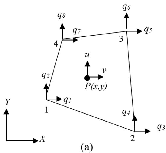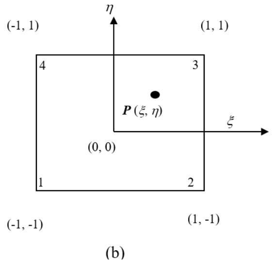 Figure 1: a) Four-node quadrilateral element; b) The quadrilateral element in $\xi$, $\eta$ space (master element) All the four shape functions can be expressed as follows: $$ N _ {1} = \frac {1}{4} (1 - \xi) (1 - \eta) \quad N _ {2} = \frac {1}{4} (1 + \xi) (1 - \eta) $$ $$ N _ {3} = \frac{1}{4} (1 + \xi) (1 + \eta) \quad N _ {4} = \frac{1 }{4} (1 - \xi) (1 + \eta) \tag{4} $$ When addressing the appropriate boundary conditions and formulating the equilibrium equations, the penalty approach was employed. As a result, the equilibrium equations can be derived by minimizing the potential energy $\varPi$ with respect to $Q$, while subjecting to the boundary conditions. These boundary conditions typically take the form of: $$ Q _ {p 1} = a _ {1}, Q _ {p 2} = a _ {2}, \dots \dots \dots , Q _ {p r} = a _ {r} \tag {5} $$ where, $\mathbf{P}_1, \mathbf{P}_2, \dots, \mathbf{P}_r$ are denoted to be the degrees of freedom and $r$ is judged to be the number of supports in the structure. The requirement that the potential energy $\Pi$ takes on a minimum value is obtained from the equation. $$ \frac{d\Pi}{dQ_i}=0\,i=2,3,\dots,N $$ By applying these specified boundary conditions and utilizing Equation (6), the finite element equations can be presented in matrix form as follows: $$ [ K ] \{Q \} = \{F \} \tag {7} $$ where, $[K]$ and $\{F\}$ are the modified stiffness and load matrices. For matrix solving, conjugate gradient method was used. Equation (7) can be resolved for the displacement vector $\{Q\}$ through Gaussian elimination. Given that the $[K]$ matrix is nonsingular, the boundary condition can be considered of specified properly. Once $\{Q\}$ has been determined, the element stress can be evaluated using the equation derived from Hooke's law, $$ \{\sigma \} = [ E ] [ B ] \{q \} \tag {8} $$ where $[B]$ is the element strain-displacement matrix and $\{q\}$ is the element displacement vector for each element, which is extracted from $\{Q\}$, using element connectivity information. The von-Mises stress offers a unified depiction of various stresses, encompassing normal stress in two directions and the corresponding shear stress, present at a particular point in case of a two-dimensional problem. When the von-Mises stress exceeds the material's yield strength, it results in yielding at that location. Likewise, if the von-Mises stress surpasses the ultimate strength, it leads to material rupture at that point. According to the failure criterion, the von-Mises stress $(\sigma_{mises})$ must be less than the material's yield stress $(\sigma_{Y})$. This criterion can be expressed in an inequality form as follows: $$ \sigma_ {m i s e s} \leq \sigma_ {Y} $$ The von-Mises stress $\sigma_{mises}$ is given by, $$ \sigma_ {m i s e s} = \sqrt {\left(\sigma_ {x} + \sigma_ {y}\right) ^ {2} - 3 \left(\sigma_ {x} \sigma_ {y} - \tau_ {x y} ^ {2}\right)} \tag {9} $$ ## III. MESH GENERATION An integral phase of the finite element method in numerical computation entails the process of mesh generation. Mesh generation involves creating a polygonal or polyhedral mesh that closely approximates a given geometric domain. In this procedure, the task is to take a domain, which can be a polygon or polyhedron (in more intricate scenarios, even domains with curved boundaries), and partition it into simple "elements" that interconnect in clearly defined manners. While striving for a minimal number of elements, certain regions within the domain may require smaller elements to enhance computation accuracy. Additionally, all these elements should possess characteristics that render them "well shaped," though the precise definition of this term may vary depending on the specific context and often relates to constraints on element angles or aspect ratios. Figure 2 provides some illustrative examples of mesh generation. 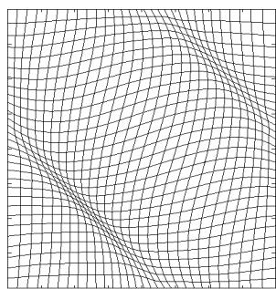  Figure 2: Some examples of mesh generation ### a) Structured mesh A structured mesh, as depicted in Figure 3, is characterized by a uniform distribution of adjacent elements around all interior nodes. Typically, such meshes are produced using structured grid generators, resulting in meshes composed entirely of quadrilateral or hexahedral elements. The algorithms employed in this process often incorporate intricate iterative smoothing methods, aimed at aligning elements with domain boundaries or physical structures. In cases where complex boundaries are involved, "block structured" techniques can be employed, allowing users to divide the domain into topological blocks. Structured grid generators find prominent application in the field of Computational Fluid Dynamics (CFD), where precise element alignment is often a requirement imposed by the analysis code or essential for capturing specific physical phenomena. 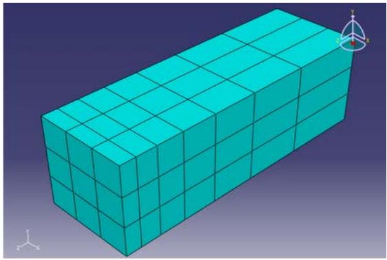 Figure 3: Structured mesh ### b) Mesh generation techniques In this section, techniques for generating meshes are considered, using triangular elements (with three nodes) and quadrilateral elements (with four nodes), specifically focusing on two-dimensional linear elements. While the analysis primarily employs a quadrilateral mesh, it's worth noting that triangles can be further subdivided into quadrilaterals, as illustrated in Figure 4. Consequently, understanding the generation of triangular elements holds significance and relevance, as it offers the possibility of transforming a triangular mesh into a quadrilateral one. 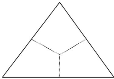 Figure 4: A triangular element is converted into three quadrilateral elements ## IV. OBJECT-ORIENTED CONCEPTS In recent years, there has been a growing interest in incorporating object-oriented concepts into finite element programming. One of the primary benefits of embracing an object-oriented approach is the simplicity and naturalness with which programs can be expanded, with minimal impact on existing code. This greatly enhances the reusability of code. Additionally, in comparison to traditional structured programming, the utilization of OOP facilitates a closer alignment between theoretical principles and their computer implementation. OOP proves especially advantageous when developing extensive and intricate programs, such as finite element systems designed to accommodate diverse element types, constitutive models, and analysis algorithms. Nevertheless, to fully leverage the advantages of the object-oriented approach, it is imperative to have a comprehensive understanding of the methodology employed and to invest substantial effort in organizing the program effectively. The objective of this research is to introduce an ongoing initiative aimed at developing a finite element analysis system based on object-oriented programming, known as FEMOOP, which encompasses the system's overall architecture. ## V. FINITE ELEMENT PROGRAMMING Prior to delving into the organizational structure of the FEMOOP program, it is essential to grasp that nonlinear finite element analysis involves computations on three distinct levels: the structural level, the elemental level, and the integration point level. At the structural (or global) level, a range of algorithms is applied to address the problem, including linear static, linearized buckling, linear dynamic, nonlinear path-following, and nonlinear dynamic analyses. These algorithms are executed using global vectors and matrices and are not reliant on the specific types of elements and materials employed in the analysis. The elemental level primarily concentrates on the calculation of elemental vectors and matrices, such as the internal force vector and stiffness matrix. These calculations are crucial for assembling the global vectors and matrices that the analysis algorithms use. Importantly, the computation of these elemental vectors and matrices remains entirely independent of the chosen analysis algorithm. The interconnection between the global and elemental levels functions in two directions. In the upward direction, global vectors and matrices are computed by amalgamating contributions from individual elements. In the downward direction, element displacements are extracted from the global displacement vector. These communication tasks are based on nodal degrees of freedom and element connectivity. Finally, at the integration point level, the computation of stress vectors and tangent constitutive matrices occurs. These quantities are utilized in the computation of elemental vectors and matrices. However, they do not depend on the specific element formulation if the essential input data for stress computation, such as strain components, are provided. Previous research has extensively investigated the convergence properties of two-dimensional solutions for elastic continuum problems using both quadrilateral and triangular elements. Those studies have identified several key factors that influence the convergence characteristics of finite element solutions. These factors encompass the fundamental shape of the elements, element distortion, polynomial order of the elements, completeness of polynomial functions, integration techniques, and material incompressibility. The flow chart of the developed program is shown in Figure 5. 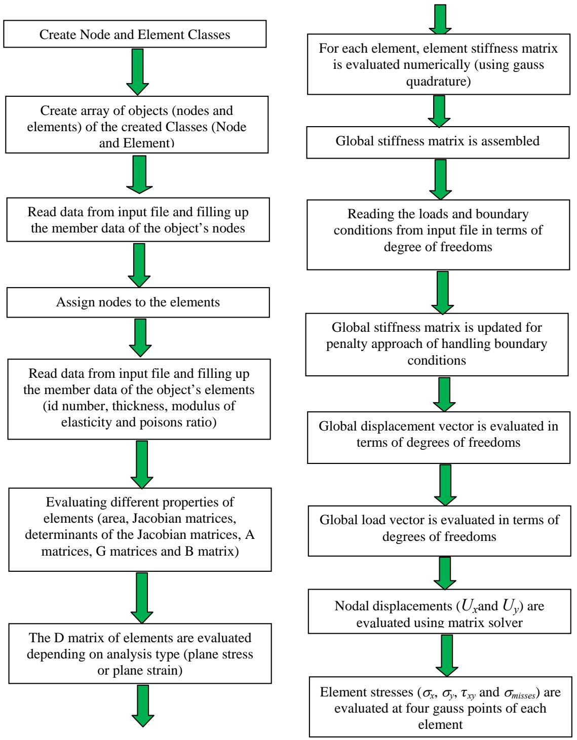 Figure 5: Flow chart of the developed program In general, it is widely recognized that quadrilateral elements outperform simplex triangular elements. Quadrilateral elements are favored for two-dimensional meshes due to their higher accuracy and efficiency, while hexahedral elements are preferred for three-dimensional meshes. This preference is evident in structural analysis and extends to various engineering disciplines. Nevertheless, it is also mentioned that triangular elements, especially those with higher-order displacement assumptions, can deliver acceptable accuracy and convergence characteristics. However, a notable drawback of triangular elements is the potential for mesh locking due to material incompressibility. This issue represents a significant limitation when employing triangular elements in certain applications. A brief overview of the object-oriented code utilized in this research is presented here. The code itself is structured around the creation of two distinctive classes, namely "Node" and "Element." Within the "Node" class, a spectrum of attributes, including coordinates, displacements, boundary constraints, and loads, is encapsulated, and the duty of reading and computing these attributes falls upon its member functions. Similarly, the "Element" class hosts an array of attributes, encompassing constituent nodes, element thickness, and material characteristics. Its member functions are thoughtfully tailored to handle the retrieval and computation of these specific properties. Subsequently, the code gives rise to an array of objects, each derived from these meticulously crafted classes. This ensemble of objects harmoniously converges to enable the creation of the global stiffness matrix and global load vector, pivotal components in the realm of finite element analysis. In addressing boundary conditions, the code adopts the penalty approach, skillfully integrating these constraints into the calculations. In this manner, the code progresses to evaluate nodal displacements and elemental stresses, completing its comprehensive analysis. ## VI. RESULTS AND DISCUSSION In this study, the SIMULIA ABAQUS 13.3 version finite element analysis software is employed for various aspects of a comprehensive finite element analysis. This encompasses pre-processing tasks like modeling, the actual processing or finite element analysis, and post-processing activities, which involve generating reports, images, animations, and other output files. The finite element analysis software allows for pre-processing, post-processing, and monitoring the solver's progress. Within this investigation, issues related to plane stress analysis, particularly concerning structural members, were explored. These investigations were conducted with appropriate boundary conditions and loadings using the finite element analysis software. To present the findings, images and a report file generated by the finite element analysis program were employed. The output file produced by the developed program was used to analyze two-dimensional plane stress problems. The primary focus lies on examining normal stresses, shear stress, and von-Mises stress at the four integration points, which represent the most vulnerable areas of structural components. Consequently, the stress data obtained from the developed program is compared with that from the finite element analysis software. The level of accuracy or deviation in these results was also quantified and presented. A two-dimensional plane stress problem is shown in Figure6. In this problem, the objective is to fabricate a basic bracket section using a steel plate with a thickness of 20 mm. The plate is fixed at the two smaller holes on the left and subjected to a load applied at the larger hole on the right. 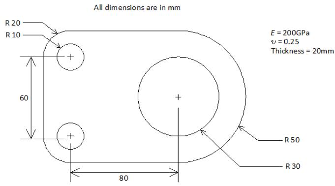 Figure 6: Bracket plate The relevant parameters employed in this problem include: Concentrated force applied Thickness of the plates Modulus of Elasticity Poisson's ratio Smaller hole radius Larger hole radius $F = 1000\mathrm{N}$ $t = 20\mathrm{mm}$ $E = 200 \times 10^{3} \mathrm{~N} / \mathrm{mm}^{2}$ $\upsilon = 0.25$ $R_{I} = 10\mathrm{mm}$ $R_{2} = 30\mathrm{mm}$ 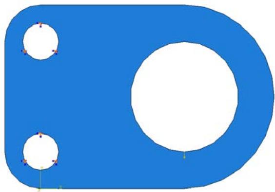 (a) 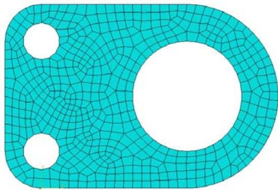 (b) Figure 7: a) Application of boundary conditions and loadings (bracket plate); b) Quadrilateral mesh (bracket plate) Figure 7(a) depicts the illustrated boundary conditions and applied loads. In this representation, the plate is securely fixed at the two small holes on the left, preventing any movement in both the x and y directions ( $Ux = Uy = 0$ ). Additionally, a concentrated force of $1000\mathrm{N}$ is applied downwards at the lowest point within the larger hole on the right. For this model, which comprises 614 nodes and 539 quadrilateral elements, the quadrilateral mesh that has been generated is showcased in Figure 7(b). The FEM analysis of the model in terms of $\sigma_{\mathrm{mises}}$ (von-Mises stress) is illustrated in Figure 8. It is observed that the von-Mises stress is maximum around the region of element no. 194 and 56, particularly near the node no. 27 which is shown in Figure 9. 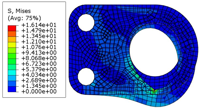 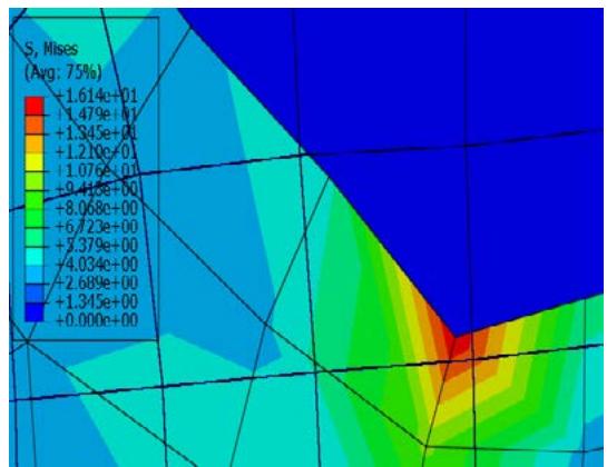Figure 8: FEM analysis of bracket plate in terms of $\sigma_{mises}$  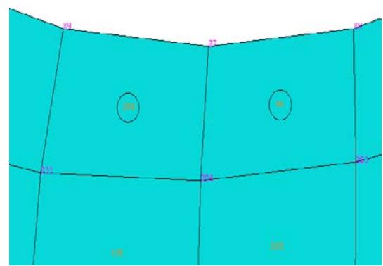 Figure 9: Location of most vulnerable region of bracket plate in terms of $\sigma_{mises}$ By employing the developed program designed for plane stress analysis, an output file has been generated for the bracket plate section, which includes stress values at the four integration points and displacement data at the nodal points. Figure 9 clearly illustrates that the maximum von-Mises stresses occur within two specific elements: element no. 194, comprising nodes 27, 89, 204, and 231, and element no. 56, composed of nodes 27, 88, 203, and 204. Comparison of $\sigma_{misses}$, $\sigma_x$, $\sigma_y$, and $\tau_{xy}$ for element no. 194 and 56 at the four integration points, and $U_x$ and $U_y$ for element no. 194 and 56 at their four nodal points obtained from the developed program and the analysis are shown in Table 1 to Table 6. Table 1: Comparison of ${\sigma }_{\text{misses }}$ for a bracket plate section <table><tr><td>Element No.</td><td>Integration point (Node No.)</td><td>σmisses from developed program (MPa)</td><td>σmisses from analysis (MPa)</td><td>% of error</td></tr><tr><td rowspan="4">194</td><td>1 (204)</td><td>9.507</td><td>9.506</td><td>0.002</td></tr><tr><td>2 (27)</td><td>12.100</td><td>12.100</td><td>0</td></tr><tr><td>3 (89)</td><td>7.309</td><td>7.308</td><td>0.002</td></tr><tr><td>4 (231)</td><td>3.696</td><td>3.691</td><td>0.005</td></tr><tr><td rowspan="4">56</td><td>1 (27)</td><td>12.526</td><td>12.525</td><td>0.002</td></tr><tr><td>2 (204)</td><td>9.372</td><td>9.370</td><td>0.002</td></tr><tr><td>3 (203)</td><td>2.387</td><td>2.381</td><td>0.007</td></tr><tr><td>4 (88)</td><td>6.425</td><td>6.423</td><td>0.002</td></tr></table> Table 2: Comparison of ${\sigma }_{x}$ for a bracket plate section <table><tr><td>Element No.</td><td>Integration point (Node No.)</td><td>σxfrom developed program (MPa)</td><td>σxfrom analysis (MPa)</td><td>% of error</td></tr><tr><td rowspan="4">194</td><td>1 (204)</td><td>-4.089</td><td>-4.086</td><td>0.004</td></tr><tr><td>2 (27)</td><td>-7.117</td><td>-7.117</td><td>0</td></tr><tr><td>3 (89)</td><td>-4.884</td><td>-4.883</td><td>0.001</td></tr><tr><td>4 (231)</td><td>-2.095</td><td>-2.091</td><td>0.005</td></tr><tr><td rowspan="4">56</td><td>1 (27)</td><td>-8.541</td><td>-8.541</td><td>0</td></tr><tr><td>2 (204)</td><td>-5.227</td><td>-5.225</td><td>0.003</td></tr><tr><td>3 (203)</td><td>-2.705</td><td>-2.700</td><td>0.006</td></tr><tr><td>4 (88)</td><td>-5.916</td><td>-5.915</td><td>0.001</td></tr></table> Table 3: Comparison of ${\sigma }_{y}$ for a bracket plate section <table><tr><td>Element No.</td><td>Integration point (Node No.)</td><td>σyfrom developed program (MPa)</td><td>σyfrom analysis (MPa)</td><td>% of error</td></tr><tr><td rowspan="4">194</td><td>1 (204)</td><td>-7.929</td><td>-7.927</td><td>0.003</td></tr><tr><td>2 (27)</td><td>-8.169</td><td>-8.168</td><td>0.002</td></tr><tr><td>3 (89)</td><td>-0.610</td><td>-0.603</td><td>0.008</td></tr><tr><td>4 (231)</td><td>-0.748</td><td>-0.741</td><td>0.010</td></tr><tr><td rowspan="4">56</td><td>1 (27)</td><td>-10.766</td><td>-10.765</td><td>0.002</td></tr><tr><td>2 (204)</td><td>-9.630</td><td>-9.629</td><td>0.002</td></tr><tr><td>3 (203)</td><td>-1.155</td><td>-1.149</td><td>0.010</td></tr><tr><td>4 (88)</td><td>-1.951</td><td>-1.948</td><td>0.005</td></tr></table> Table 4: Comparison of ${\tau }_{xy}$ for a bracket plate section <table><tr><td>Element No.</td><td>Integration point (Node No.)</td><td>τxy from developed program (MPa)</td><td>τxy from analysis (MPa)</td><td>% of error</td></tr><tr><td rowspan="4">194</td><td>1 (204)</td><td>-3.795</td><td>-3.795</td><td>0</td></tr><tr><td>2 (27)</td><td>-5.390</td><td>-5.389</td><td>0.001</td></tr><tr><td>3 (89)</td><td>-3.275</td><td>-3.272</td><td>0.004</td></tr><tr><td>4 (231)</td><td>-1.851</td><td>-1.849</td><td>0.004</td></tr><tr><td rowspan="4">56</td><td>1 (27)</td><td>4.472</td><td>4.471</td><td>0.001</td></tr><tr><td>2 (204)</td><td>2.457</td><td>2.456</td><td>0.002</td></tr><tr><td>3 (203)</td><td>0.237</td><td>0.229</td><td>0.047</td></tr><tr><td>4 (88)</td><td>2.162</td><td>2.159</td><td>0.006</td></tr></table> Table 5: Comparison of $U_{x}$ for a bracket plate section <table><tr><td>Element No.</td><td>Node No.</td><td>Uxfrom developed program (mm)</td><td>Uxfrom analysis (mm)</td><td>% of error</td></tr><tr><td rowspan="4">194</td><td>204</td><td>-0.00032</td><td>-0.00032</td><td>0</td></tr><tr><td>27</td><td>-0.00017</td><td>-0.00016</td><td>0.001</td></tr><tr><td>89</td><td>0.00001</td><td>0.00001</td><td>0</td></tr><tr><td>231</td><td>-0.00028</td><td>-0.00028</td><td>0</td></tr><tr><td rowspan="4">56</td><td>27</td><td>-0.00017</td><td>-0.00017</td><td>0</td></tr><tr><td>204</td><td>-0.00032</td><td>-0.00032</td><td>0</td></tr><tr><td>203</td><td>-0.00035</td><td>-0.00034</td><td>0.001</td></tr><tr><td>88</td><td>-0.00032</td><td>-0.00031</td><td>0.001</td></tr></table> Table 6: Comparison of $U_{y}$ for a bracket plate section <table><tr><td>Element No.</td><td>Node No.</td><td>\(U_y \) from developed program (mm)</td><td>\(U_y \) from analysis (mm)</td><td>% of error</td></tr><tr><td rowspan="4">194</td><td>204</td><td>-0.00308</td><td>-0.00308</td><td>0</td></tr><tr><td>27</td><td>-0.00325</td><td>-0.00325</td><td>0</td></tr><tr><td>89</td><td>-0.00259</td><td>-0.00259</td><td>0</td></tr><tr><td>231</td><td>-0.00254</td><td>-0.00253</td><td>0.001</td></tr><tr><td rowspan="4">56</td><td>27</td><td>-0.00325</td><td>-0.00324</td><td>0.001</td></tr><tr><td>204</td><td>-0.00308</td><td>-0.00307</td><td>0.001</td></tr><tr><td>203</td><td>-0.00320</td><td>-0.00310</td><td>0.001</td></tr><tr><td>88</td><td>-0.00316</td><td>-0.00316</td><td>0</td></tr></table> In the context of the bracket plate section, the regions of maximum stress vulnerability are identified as element no. 194, defined by nodes 27, 89, 204, and 231, and element no. 56, characterized by nodes 27, 88, 203, and 204. Consequently, a comparative analysis is conducted to assess the stress distributions at the four integration points and the displacements at the nodal points for both element no. 194 and element no. 56 within the above-mentioned model. Table 1 displays the $\sigma_{misses}$ values, indicating that the maximum tensile stress is located at integration point 1 for element no. 56. The calculated stress is $12.526\mathrm{MPa}$ from the developed program and $12.525\mathrm{MPa}$ from the analysis, resulting in near-identical values with a minimal deviation of only $0.002\%$. A comprehensive examination of all the values in Table 1 reveals consistently minimal error percentages in the $\sigma_{misses}$ results. The findings regarding $\sigma_{misses}$ from previous studies demonstrated a high degree of similarity (Hoque, 2016; Hoque and Islam, 2023). When examining $\sigma_{x}$ in Table 2, it becomes apparent that the maximum compressive stress is located at integration point 1 for element no. 56. This stress measures $8.541\mathrm{MPa}$, which is identical when derived from both the developed program and the analysis, resulting in a perfect match with zero percentage of error. Upon reviewing all the other $\sigma_{x}$ values in Table 2, it is evident that the results are consistently in close agreement, displaying only minimal error percentages. Table 3 illustrates $\sigma_{y}$, where the maximum compressive stress is identified at integration point 1 for element no. 56. This stress registers at $10.766\mathrm{MPa}$ from the developed program and $10.765\mathrm{MPa}$ from the analysis, showcasing remarkably similar values with a minuscule deviation of only $0.002\%$. A thorough examination of all the other $\sigma_{y}$ values in Table 3 reveals consistently close results with exceedingly small percentages of error. In the case of $\tau_{xy}$, as demonstrated in Table 4, an intriguing pattern are observed. Firstly, the maximum compressive stress occurs at integration point 2 for element no. 194, measuring $5.390\mathrm{MPa}$ in the developed program and $5.389\mathrm{MPa}$ in the analysis. These two values are remarkably similar, differing by a mere $0.001\%$ margin. Secondly, the maximum tensile stress manifests at integration point 1 for element no. 56, with values of $4.472\mathrm{MPa}$ computed by the developed program and $4.471\mathrm{MPa}$ from the analysis. Impressively, these tensile stress values exhibit a near-identical match, showing only a minimal $0.001\%$ disparity. Delving further into Table 4, it becomes evident that $\tau_{xy}$ values demonstrate a high degree of consistency, with errors consistently remaining relatively small. Previous research (Hoque, 2016; Hoque and Islam, 2023) revealed a remarkable level of similarity in their findings regarding $\tau_{xy}$. In the context of displacement analysis, an examination of $U_{x}$ reveals interesting insights, as depicted in Table 5. The maximum displacement is pinpointed at node no. 203 within element no. 56, measuring $0.00035 \mathrm{~mm}$ according to the developed program and $0.00034 \mathrm{~mm}$ as per the analysis. These two values exhibit remarkable proximity, differing by just $0.001\%$, emphasizing their substantial agreement. Similarly, when investigating $U_{y}$, as presented in Table 6, the maximum displacement is found at node no. 27 of element no. 56. This displacement is quantified at $0.00325 \mathrm{~mm}$ through the developed program and $0.00324 \mathrm{~mm}$ through the analysis, showcasing a close match with a mere $0.001\%$ variation. From the comprehensive comparison of all other values within Table 5 and Table 6, it becomes evident that the results for both $U_{x}$ and $U_{y}$ consistently maintain a relatively tight margin of error, underlining their close agreement. The maximum von-Mises stress concentrations are notably located around element no. 194 and 56, particularly in the proximity of node no. 27, as depicted in Figure 9. Employing a developed program for plane stress analysis, an output file is generated, which details the stress values at the four integration points for a bracket plate section. Figure 9 vividly illustrates that the maximum von-Mises stresses manifest within two specific elements: element no. 194, encompassing nodes 27, 89, 204, and 231; and element no. 56, comprising nodes 27, 88, 203, and 204. Comparative data for $\sigma_{mises}$, $\sigma_x$, $\sigma_y$, and $\tau_{xy}$ for element no. 194 and 56 at the four integration points, as obtained from both the developed program and finite element analysis software, are presented in Table 1 through Table 4. For instance, when node no. 27 of element no. 56 is examined, the von-Mises stress registers at 12.526 MP a based on the developed program (theoretical). This von-Mises stress results from the combination of all stresses acting at that specific location, namely normal stresses in two-directions and shear stress. For node no. 27 of element no. 56, the normal stresses along the x and y directions, as well as the shear stress, are determined to be -8.541 MP a, -10.766 MP a, and 4.472 MP a, respectively. Utilizing these values for normal and shear stresses and applying Equation (9), a von-Mises stress of 12.526 MP a is obtained through theoretical calculations, which closely aligns with the analysis-derived von-Mises stress of 12.525 MP a, representing a mere $0.002\%$ deviation. When comparing von-Mises stress values for other nodes (node no. 88, 203, 204) of element no. 56 and nodes (node no. 27, 89, 204, and 231) of element no. 194 between the developed program and analysis results, only minimal discrepancies are observed, typically ranging from $0\%$ to $0.007\%$. Therefore, it can be said that the results from the developed program closely align with the analysis outcomes. The material employed for the bracket plate section is steel, having a yield strength of $250\mathrm{MPa}$. According to the von-Mises stress criterion, it is imperative that von-Mises stress does not exceed the material's yield strength, as surpassing this limit would lead to material yielding and failure. The von-Mises stress values obtained both from the developed program and the analysis, for the four nodes (node no. 27, 88, 203, and 204) of element no. 56 and the remaining four nodes (node no. 27, 89, 204, and 231) of element no. 194, all fall within the range of the material's yield strength. Consequently, it can be said that the bracket plate section will not yield or fail when subjected to a concentrated downward force acting at its lowest point (within the larger hole on the right side of the bracket plate section). To visualize the generated mesh for a bracket plate section, a specialized two-dimensional mesh viewer program has been developed using the Python programming language. The program provides a graphical representation of the mesh structure. In Figure 10, the outcomes of this endeavor can be observed, specifically focusing on the resultant quadrilateral mesh for a bracket plate section. These intricate mesh structures have been systematically generated, guided by the magnification factor meticulously calculated through the Python program. Furthermore, the utilization of the developed mesh viewer program extends to the visualization of the triangular mesh within the bracket plate section. Figure 11 provides an illustrative representation of the resulting triangular mesh for this specific model, generated through the combined efforts of ABAQUS software and the developed mesh viewer program. 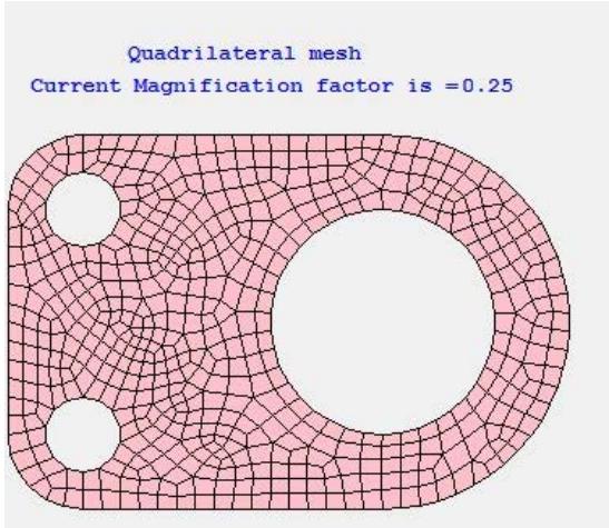 Figure 10: Quadrilateral mesh obtained by using the developed mesh viewer program for a bracket plate section 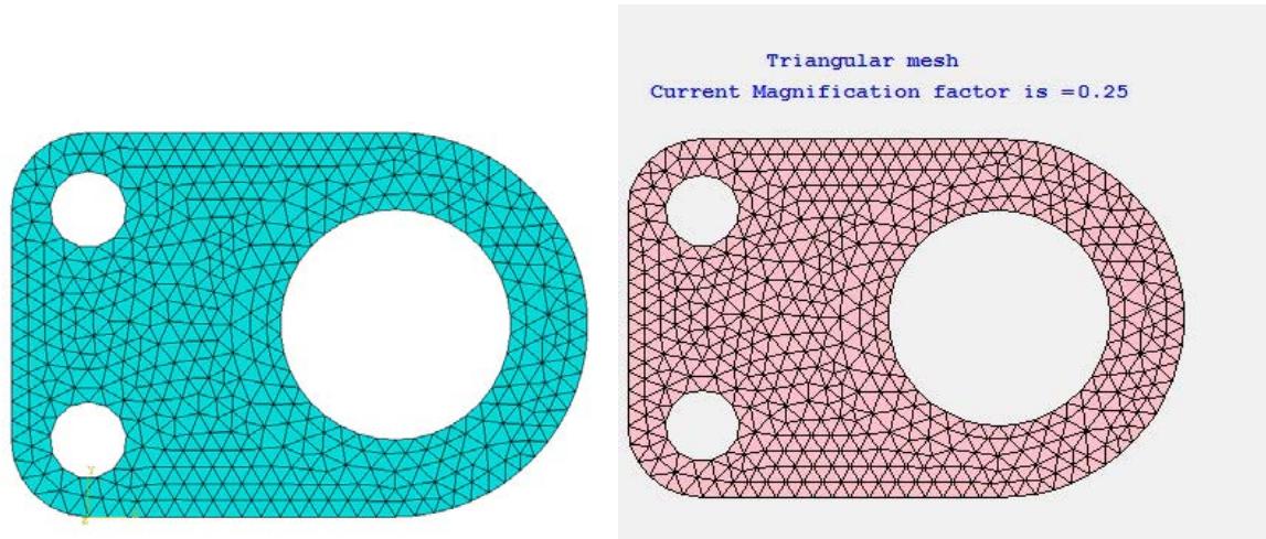 Figure 11: Triangular mesh for a bracket plate section via using the a) ABAQUS software; b) developed mesh viewer program ## VII. CONCLUSIONS The conclusions that can be made from this study are summarized below: - An efficient and reliable object-oriented program has been developed to handle two-dimensional four-node quadrilateral elements. This program facilitates precise stress value calculations at the four integration points (gauss points) for bracket plate sections that include structural discontinuities. It serves as an invaluable tool for analyzing a diverse array of two-dimensional plane stress problems, greatly improving the efficiency and accuracy of the analysis process. - The program developed for the assessment of the structural sections' most vulnerable areas has undergone successful validation of its analysis results. Upon meticulous comparison of stress values at each gauss point and displacement values at nodal points, it became evident that the program's analysis results displayed merely marginal percentages of error. This underscores the remarkable precision and reliability achieved by the developed program. - The mesh viewer program that has been developed possesses the capability to visualize meshes of both quadrilateral and triangular configurations, with the added flexibility to adjust the magnification factor as required for different models associated with structural sections. ### ACKNOWLEDGEMENTS The authors would like to express their sincere gratitude to all the individuals who have provided their valuable support, both directly and indirectly, throughout various phases of this project. Furthermore, the authors would like to highlight the UGC HEQEP Sub Project "Strengthening the Research Capabilities and Experimental Facilities in the Field of Marine Structure" (CP#3131), which has significantly contributed to the enhancement of the simulation lab facilities.

Generating HTML Viewer...

References

21 Cites in Article
J Baugh,D Rehak (1990). Computational abstractions for finite element programming.
G Baumann (1997). Linear structural stress analysis of a hull girder penetration and a short longitudinal bulkhead using finite element modeling.
R Bea,E Cramer,R Schulte-Strauthaus,R Mayoss,K Gallion,K Ma,R Holzman,L Demsetz (1995). Ship's Maintenance Project. Conducted at University of California.
Thierry Gafner (1992). Analyse critique des méthodes classiques et nouvelle approche par la programmation mathématique en classification automatique.
Yves Dubois-Pèlerin,Thomas Zimmermann,Patricia Bomme (1992). Object-oriented finite element programming: II. A prototype program in smalltalk.
Anders Sellman,Per Katzman,Sten Andreasson,Magnus Löndahl (2013). Long-term effects of hyperbaric oxygen therapy on visual acuity and retinopathy.
Gregory Fenves (1990). Object-oriented programming for engineering software development.
B Forde,R Foschi,S Stiemer (1990). Object-oriented finite element analysis.
Kazi Hoque,Md. Islam (2023). Stress-strain analysis of structural discontinuities associated with ship hulls.
Kelley L Breeden,J Louda (2020). Microcystis Aeruginosa Needs a Microbiome in Order to Utilize Phosphorus from Organo-Phosphates.
Aevelina Rahman,Md. Karim (2016). Green Shipbuilding and Recycling: Issues and Challenges.
J Mackerle (1996). Object-oriented techniques in FEM and BEM. a bibliography.
L Martha (2002). An object-oriented framework for finite element programming.
G Miller (1991). An object-oriented approach to structural analysis and design.
M Niu (1998). Airframe Structural Design.
F Presuel-Moreno,K Hoque,A Rosa-Pagan (2020). Corrosion propagation monitoring using galvanostatic pulse on reinforced concrete legacy samples.
F Presuel-Moreno,K Hoque (2019). Corrosion propagation of carbon steel rebar embedded in concrete.
F Presuel-Moreno,M Nazim,F Tang,K Hoque,R Bencosme (2018). Corrosion propagation of carbon steel rebars in high performance concrete.
C Soares,Y Garbatov (1998). Reliability of maintained ship hull girders subjected to corrosion and fatigue.
S Thohura,M Islam (2013). Study of the effect of finite element mesh quality on stress concentration factor of plates with holes.
T Zimmermann,Y Dubois-Pelerin,P Bomme (1992). Object-oriented finite element programming.
No ethics committee approval was required for this article type.
Data Availability
Not applicable for this article.
How to Cite This Article
Kazi Naimul Hoque. 2026. \u201cAn Object-Oriented Finite Element Programming Approach to Analyze Structural Discontinuities of A Bracket Plate Section\u201d. Global Journal of Science Frontier Research - F: Mathematics & Decision GJSFR-F Volume 23 (GJSFR Volume 23 Issue F7).
Explore published articles in an immersive Augmented Reality environment. Our platform converts research papers into interactive 3D books, allowing readers to view and interact with content using AR and VR compatible devices.
Your published article is automatically converted into a realistic 3D book. Flip through pages and read research papers in a more engaging and interactive format.
Our website is actively being updated, and changes may occur frequently. Please clear your browser cache if needed. For feedback or error reporting, please email [email protected]
Thank you for connecting with us. We will respond to you shortly.