## I. MAIN TEXT ### INTRODUCTION The peculiarity of the control of an asynchronous electric drive (ED) is the need to ensure the rotor flux coupling of an induction motor (IM) to ensure the necessary electromechanical torque of the motor. With the correct solution of this problem, an asynchronous ED in terms of its dynamic properties approaches a direct current ED with independent excitation. During scalar control of an asynchronous ED, the rotor flux is formed due to the functional dependence of the IM voltage on the frequency with possible consideration of the current. With vector control - due to the direct and inverse transformation of the coordinate system of the current and voltage vectors of the frequency converter (FC) with the selection of active and reactive components of the current relative to the FC voltage and relative to the EMF of the rotor and the regulation of signals proportional to the ED speed and rotor flux coupling [1-3]. The error in determining the rotorflux coupling depends on the error entered for the calculations of the internal inductances and resistances of the IM, especially on the resistances of the stator and rotor, which are subject to temperature changes. This error can significantly worsen the ED characteristics, in particular, limit the speed control range from below due to the impossibility of creating the necessary electromagnetic moment at low IM rotation frequencies. To improve the characteristics of the ED, an observer is used, which automatically monitors the change in IM parameters, which depend on the accuracy of determining the components of the current relative to the EMF and the signals that determine the IF voltage and the speed of the ED. The existence of many types of observers [2] speaks of the problem of taking into account changes in IM parameters. High-quality monitoring requires high computing capabilities of microprocessor control systems of FC for ED. To track the time constant of the rotor, which can change during the operation of the ED due to the temperature change of the active resistance of the rotor, or the change in the inductance of the rotor, the reactive power of IM that is consumed is determined in work [3]. The current value of the rotor time constant determined in this way is subsequently used in the above forward and reverse coordinate transformation to control the stator current, rotor flux coupling and ED as a whole. Considering that the reactive power is uniquely related to the rotorflux coupling and in the steady state does not depend on the resistances of the stator and rotor, it is possible to simplify the task of controlling the ED by determining the rotorflux coupling and the speed of the ED through the reactive power [4]. The purpose of the work is to consider the features of the practical use of the method of controlling an asynchronous ED, which is based on the measurement of the reactive power consumed by the IM. Presentation of the main material. Based on the expressions given in [3], the relationship between the rotor flux coupling and the instantaneous reactive power of IM can be written in the form: $$ \bar{U}_{S} \times \bar{I}_{S} = I_{S}^{2} \omega \sigma L_{S} + \frac{\omega_{\Psi} \Psi_{r}^{2}}{L_{r}} + \frac{\omega_{r}}{R_{r}} \frac{d\Psi_{r}}{dt} \Psi_{r}, $$ where each term without taking into account the proportionality factor means the following: $\bar{U}_S x \bar{I}_S$ - the vectors product of the stator voltage $\bar{U}_S$ and current $\bar{I}_S$, which determines the instantaneous reactive power (the full instantaneous reactive power of IM is 3/2 times more); $I_S^2 \omega \sigma L_S$ -reactive power on the dissipation inductance $\sigma L_S$ of the stator phase, $I_S$ - modulus of vector $\bar{I}_S$; $\frac{\omega_\Psi \Psi_r^2}{L_r}$ - reactive power on the inductance of the rotor; $\Psi_r$ -moduleof the vector of the rotor flux; $\frac{\omega_r}{R_r}\frac{d\Psi_r}{dt}\Psi_r^-$ is the dynamic component of reactive power. Relating to the stator the resistance and inductance of the entire circuit between the FC and IM, the product of the stator voltage and current vectors can be given as the product of the FC voltage and current vectors $\bar{U} x\bar{I}$. By plotting the FC voltage and current vectors in the rotating orthogonal coordinate system oriented by voltage, the product of the voltage and current vectors can be defined as the product of the FC voltage $U$ and the reactive component of the FC current $I_{xU}$ relative to this voltage: $\bar{U} x\bar{I} = UI_{xU}$, where $I_{xU} = I\sin \varphi$, $\varphi$ is the angle between voltage and current vectors. The value of the current $I_{xU}$ at the angle $\theta_U$, which is counted from the moment of the phase A transition of the FC voltage from minus to plus (also the angle of rotation of the rotating coordinate system), can be found using the coordinate transformation formula $$ I_{XU} = -i_a \sin \theta_U - \frac{1}{\sqrt{3}} (i_a + 2i_c) \cos \theta_U , $$ where ia, ic are the instantaneous value of the currents of phases A and C at the moment of current measurement at the angle $\theta_{U}$. Finding the active component of the current relative to the voltage $I_{RU} = I\cos \varphi$ according to the formula $$ I_{RU} = i_a \cos\theta_U - \frac{1}{\sqrt{3}} (i_a + 2i_c) \sin\theta_U, $$ the square of the full current can be determined: $$ I ^ {2} = I _ {R U} ^ {2} + I _ {X U} ^ {2}. $$ In the steady state, the dynamic component of the reactive power is zero, and the rotor flux coupling frequency $\omega \psi$ is equal to the output frequency of the FC voltage $\omega$. In this mode, expression (1) taking into account the above-mentioned re-designations takes the form: $$ U I _ {X U} = I ^ {2} \omega L _ {C} + \frac {\omega \Psi_ {r} {} ^ {2}}{L _ {r}}. \tag {4} $$ Here, $L_{C}$ is the inductance of the stator circuit, including the dissipation inductance of the stator phase $\sigma L_{S}$. Violation of this condition causes a transient process. If at the same time the FC voltage is influenced by changing the reactive power $UI_{XU}$, it is possible to reach a steady state again, in which the rotor flux coupling will correspond to the reference rotor flux $\Psi_{r^{*}}$. This influence can be carried out with the help of the FC voltage regulator. With an integral regulator according to the formula: $$ U = k _ {i n t. U} \int \left(I ^ {2} \omega L _ {C} + \frac {\omega \psi_ {r} ^ {*}}{L _ {r}} - U I _ {X U}\right) d t, \qquad (5) $$ where $k_{int,U}$ is the integral coefficient of the voltage regulator. The specified value of the flux coupling of the rotor $\Psi_{r}^{*}$ is determined by the dependence $U(f)$ of the voltage on the FC frequency $f = \omega /2\pi$. For low-frequency regulation requirements, the characteristic [5] can be used: $$ U(f) = I_{\mu *} \sqrt{R_{c}^{2} + [2\pi f(L_{c} + L_{0})]^{2}} , $$ where $R_{C}$ is the resistance of the stator circuit, $L_{o}$ is the mutual inductance of the stator and rotor; $I_{\mu}^{*}$ is the set value of the magnetization current, which can be determined through the nominal values of frequency $f_{nom}$ and voltage $U_{nom}$ according to the formula $I_{\mu}^{*} \approx U_{nom} / 2\pi f_{nom}(L_{S} + L_{o})$. (Here voltage and current are given in actual values). The voltage value $U$ is determined by the microprocessor control system as a function of all variables at a given discreteness interval, and its value at the previous discreteness interval is taken as the value of $U$ in the right part of the formula. The discreteness of calculations is determined by the modulation frequency, which in modern FCs is measured in kilohertz. As a result of the transformation of the coordinate system into a rotating system with constant variables in expression (5), the voltage $U$ is constant at all periods of discreteness. The FC voltage calculated in this way does not depend on the IM resistances, which are subject to temperature changes, and ensures that the rotor flux coupling corresponds to the set value. At frequencies close to zero, you can use the value of the reactive power for some frequency close to zero, at which the calculated error does not exceed the permissible, for example, $1\%$ of the nominal. In this way, it is possible to ensure the nominal IM torque over the entire range of speed changes, including zero. In the ED without a speed sensor, to ensure the compliance of the speed with the set value, it is necessary to take into account the IM slip, the frequency of which $f_{s}$ is proportional to the rotor current $I_{r}$. If the rotating orthogonal coordinate system is oriented not by the FC voltage, but by the flux-coupling EMF of the rotor, then the active component of the current relative to the EMF $I_{RE}$ will mean the rotor current $I_{r}$; $I_{RE} = I_{r}$. Then the sliding frequency can be found as: $$ f_{s} = \frac{1}{2\pi\Psi_{r}} R_{r} I_{RE} \tag{6} $$ and ED speed regulation should be carried out according to the formula: $$ f = f ^ {*} + f _ {s}, $$ where $f$ is the frequency of the output voltage of the inverter ( $f = 2\pi \omega$ ), $f^*$ is the reference frequency. The constancy of the rotor flux $\Psi_r$ provided by the voltage regulator, allows you to use this formula in the entire regulation range. The active component of the current relative to the EMF $I_{RE}$ can be determined from the expression for coordinate transformation, in which, unlike expression (3), instead of the angle $\theta_U$, which is independent of IM parameters, the angle $\theta_E$ is used, which is calculated from the transition of the EMF of phase A through zero. At the same time, the angle $\theta_E$, which is due to the IM parameters, depends on their change. The $I_{RE}$ current will not depend on changes in IM parameters, if it is found based on the reactive power, taking into account formula (4): $$ I_{RE} = \sqrt{ I^{2} - \frac{U I_{XU} - I^{2} \omega L_{C}}{\omega L_{r}} } \tag{7} $$ where the expression under the root is the difference of the squares of the full current and the reactive component of the current $I_{XE}$ relative to the EMF. As can be seen, there are no temperature-dependent active resistances in this expression. Thanks to the rotor flux coupling regulator, $\Psi r$ does not depend on changes in IM parameters. However according to (6), the slip frequency $f_{\mathrm{S}}$, and therefore the IM speed $\nu = f - f_{\mathrm{S}}$, at a constant current $I_{\mathrm{RE}}$ and a certain moment depend on the temperature change of the rotor resistance. Therefore, with high requirements for speed regulation accuracy, adaptation of the regulation system to changes in rotor resistance should be used or a speed regulator should be used. If full slip compensation, when $f = f^{*} + f_{s}$, is provided at some average rotor temperature, there will be overcompensation at a low temperature, and under compensation at a high temperature. When overcompensating for slippage, the possible instability of the control system should be taken into account. Thus, when overcompensating with a coefficient for an integral frequency regulator, the stability condition has the form \[6\]: $$ k < \frac{T _ {\text{int}}}{T _ {M} \left(1 + T _ {C} / T _ {\text{int}}\right)}, \tag{8} $$ where $T_{M}$ is the electromechanical time constant of ED; $T_{C}$ is the time constant of the stator circuit; $T_{int}$ is the integration time constant of the frequency control circuit. The structural diagram of the ED with reactive power control [7] is presented in Fig. 1, where CC is a coordinate converter; SS and SR - speed sensor and speed regulator; $n$, $n^*$ - speed and reference speed; Ud is the input voltage of the inverter (the circuit that provides the motor voltage $U$ regardless of the change in Ud is part of the inverter); $i_a$, $i_c$ - currents of phases A and C of the frequency converter (FC); $k_f$, $T_{int}$ - coefficient and the time constant of the frequency regulator. Functional blocks perform operations: F1 - determines the reference of the reactive power $$ Q ^ {*} = I ^ {2} \omega L _ {c} + \frac {\omega \Psi_ {r} ^ {* 2}}{L _ {r}}, $$ where $L_{c}, L_{r}$ are the stator and rotor inductances, $\Psi_{r}^{*}$ is the reference rotor flux, $\omega = 2\pi f$. F2 - determines the active component of the rotor current, according to (7). The $I_{RE}$ value is calculated without taking into account the sign. The sign of the $I_{RE}$ current depends on the specified direction of rotation of the IM and on the mode in which it operates, engine or generator. To determine the sign, you can use the expression for active power $P_{R}$: $$ P _ {R} = U I _ {R U} - I ^ {2} R _ {C}, $$ where $R_{C}$ is the resistance of the stator circuit, including the resistance of the connecting wires between the inverter and the motor. If the active power is positive, then the $I_{RE}$ is marked with a "+" if it is negative - the sign is "-" Since the active power depends on $R_{C}$, which is prone to temperature changes, it is advisable to periodically specify its value, this is possible with the output frequency of the inverter close to 0 Hz (in the frequency range of $\pm 0.1\mathrm{Hz}$ ) in a stable mode of operation: $R_{C}\approx U / I$. Taking into account their can beimplemented programmatically.technological due to the features of the electric drive, The direction of slip compensation depends on the sign of $I_{RE}$: with the "+" sign, the slip compensation increases the frequency, with the "-" sign it decreases the frequency, possibly to zero and reverse. 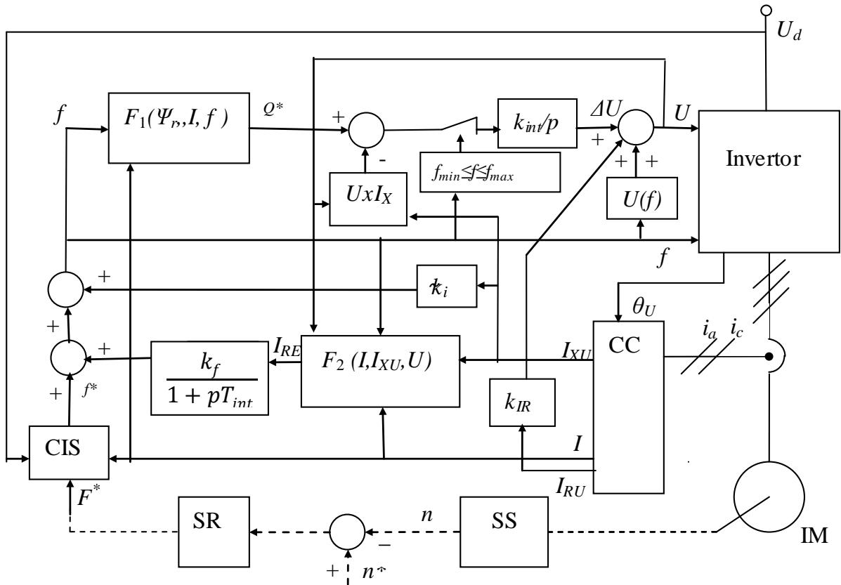 Fig. 1 #### The figure also shows: CIS is a controlled intensity setter that controls the set frequency $f^{*}$, limits the rate of change of $f^{*}$ at a high rate of change of the frequency $F^{*}$ at the input of the set intensity setter; prohibits increasing the frequency when the current $I$ exceeds the permissible value or reduces it when it is greatly exceeded; prohibits frequency reduction when the input voltage of the inverter $U_{d}$ exceeds the permissible value; $k_{IR}$ - the IR-compensation coefficient, which increases the voltage of the converter by the value of the voltage drop on the internal resistors of the AM at current I; $k_{i}$ is the feedback coefficient of the reactive component of the current to ensure the stability of the automatic control system at low FC frequencies. In the given scheme, before multiplying by $k_{i}$, the variable component of the signal $I_{XU}$ is allocated. As can be seen from the structural diagram, all the signals on the adders are marked "plus", except for the signal of the measured reactive power $UxI_{xU}$ for the reactive power regulator and the signal of the speed sensor in the presence of a speed regulator. Such a scheme provides optimal microprocessor control of the electric drive with the permitted rate of change of the speed of the electric motor. The reactive power regulator with the output signal $\Delta U$ regardless of the temperature change of the electric motor parameters provides the necessary flux coupling of the rotor to create the necessary mechanical torque of the motor over the entire speed control range, including zero speed. The structural diagram shows a comparison of the set and actual values of the reactive power and presents a variant of the regulator, when the output signal does not change in the specified frequency interval near the zero value, therefore the regulator is taken as integral, $\text{kint}$ is the coefficient of the regulator. The speed of the ED is demonstrated on the oscillogram of the reverse current at a frequency of 30 Hz in the alternating current ED EKT4R-250-380-50 with electricity recovery into the power supply network of the Zaporizhzhya Electrical Apparatus Plant, given in [7], (Fig. 2). When the frequency $f$ is reduced, there is a limitation of the speed of the frequency change according to the voltage $U_{d}$, and when the frequency is increased, there is a limitation according to the current $I$. Taking into account the limitations of the voltage and current, the reversal time is minimal. The reverse can be judged by the change in the phase alternation of the currents $i_{a}, i_{c}$. With voltage or current restrictions, the reactive power regulator does not work. But when the ED works without limiting the signals, it increases the quality of the ED due to pre-voltage regulation by the $\Delta U$ signal. A feature of a high-quality ED is the ability to work with multidirectional disturbances aimed at braking or acceleration of the engine. This is important for the electric vehicle drive, crane electric drive, metallurgical, for example, divert ingroller conveyors with a combination of acceleration and braking and other electric drives. Different polarity disturbances when working with a 30 kW engine are shown in fig. 3. At the same time, the speed is reduced to one pair of IM poles, therefore the signals of the speed $n$, the set value of the speed $n^*$, the frequency $f$, the set value of the frequency $f^*$, $F^*$ have the same scale. In the absence of a speed regulator and one pair of poles $n^* = F^*$. Values along the ordinate axes are in hertz and amperes. Voltage $U$ is reduced to frequency by multiplying by the ratio of nominal values $f_{\text{nom}} / U_{\text{nom}}$. All signals were calculated for each discreteness interval. In this case, the discreteness of the calculations is 0.5 ms, which corresponds to the microprocessor modulation frequency of 2 kHz. In practice, there may be a higher modulation frequency. This makes it possible to approximate the sinusoidal voltages of the inverter with great accuracy and to form almost inertialess regulation processes in the ED. In case of braking disturbances, in which the speed decreases, the control system increases the FC frequency, and in acceleration disturbances, in which the speed increases, it reduces the IF frequency, while ensuring the necessary IM sliding.  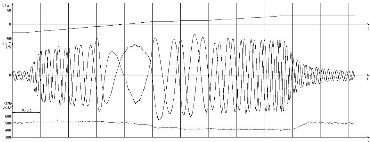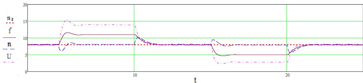 Fig. 2 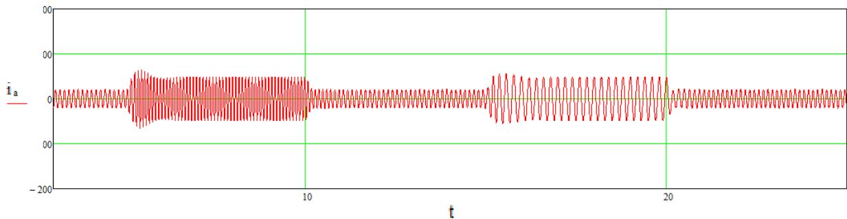 Fig. 3 The decrease and increase of sliding in the figure corresponds to the application of the nominal load moment to the electric motor in one direction or another. If there quired frequency reduction is greater than the set value of the speed, then the inverter must reverse, and the established value of the frequency after the reversal $f_{\mathbb{R}}$ must complement the set value nback to the value of the sliding frequency $f_{s}$ required for the compensation of the slip $f_{s}$: $$ f_{R} = f_{S} - n^{*}. $$ This was confirmed during testing of the electric drive and can be seen from the oscillogram obtained during mathematical modeling in fig. 4, where the set value $n^*$ gradually changes from $+1 \mathrm{~Hz}$ to $-1 \mathrm{~Hz}$ when the direction of periodic disturbances is alternately changed. Also, as in fig. 2, in fig. 4 shows two currents $i_a$, $i_c$ by alternating which it is possible to judge the direct or reverse mode of operation of the electric drive. With the second and last disturbance in fig. 4, the frequency increases as with the first disturbance in fig. 3. And with the first, third and fourth disturbances, the frequency decreases to zero and after the reversal increases to $f_{R}$. The details of the process can be seen in the figure with an enlarged time scale during the first disturbance. In the first section, the frequency decreases to zero, then reverses (on the diagram at the moment of 5,52 s), which can be seen from the change in the phase alternation of the currents ia, ic. Then the frequency increases to the value $f_{R}$ and the speed $n$ approaches the set value nback. After the end of the disturbance, the frequency of the currents decreases to zero, a reversal occurs (on the diagram at the moment 17,5 s), and the frequency increases to correspond to the set speed value. At the same time, the reverse process is continuous and inertialess, unlike similar processes in a direct current drive with separate control of bridges with three-position or scanning logic [8]. It should be borne in mind that at a frequency close to zero, the reactive component of the current decreases for the calculation of the reactive power required for controlling the ED, and the error in its determination also increases. One of the ways to determine the reactive power at a frequency close to zero is to use the value of the reactive power at the border of the interval, where the error is still satisfactory. The existing error does not mean a reduction in the speed control range, since the speed differs from the frequency due to slippage, and the speed measurement error is smaller, the greater the engine load. When the frequency is close to zero, the speed depends on the load moment of the electric motor. Thus, within the frequency interval $f_{\min} < f < f_{\max}$ (see fig. 1), where the reactive power measurement error is large, the output signal of the reactive power regulator $\Delta U$ takes the value $\Delta U(f_{\min})$ or $\Delta U(f_{\max})$, depending on whether the frequency increased in the region of negative frequencies, reaching fmin, or decreased in the region of positive frequencies, reaching fmax. The change in the load moment in the middle of the specified frequency interval can be taken into account by the corresponding change in the current $$ I = \sqrt{\frac{4}{3} \left(i_{a}^{2} + i_{ac} i_{c} + i_{c}^{2}\right)} $$ and not its active component, which is acceptable, since at low frequency the difference between them is small. (According to formulas (2, 3, 9) the amplitude values of the current and its active and reactive components are calculated). To reduce the error of determining the active and reactive current components at low frequency, and the corresponding reduction of the limited frequency interval around the zero value, their instantaneous values can be calculated not only relative to the transition time of the voltage curve of phase A of the FC from the region of negative values to the region of positive values, but also relative to time of the next transition through zero of any of the phases both from the region of negative values to the region of positive values according to expressions (2, 3), (11), (13), and from the region of positive values to the region of negative values according to expressions (10), (12), (14) with the current values of the angles $\theta_{a}, \theta_{b}, \theta_{c}$ and $\theta_{c}, \theta_{a}, \theta_{b}$, respectively. The "minus" sign in the index means that the angle is calculated from the transition of the voltage curve from a positive to a negative value. $$ i_{R} = -i_{c} \cos \theta_{-c} - \frac{1}{\sqrt{3}} (i_{a} - i_{b}) \sin \theta_{-c} $$ $$ i_{X} = -i_{c} \sin \theta_{-c} - \frac{1}{\sqrt{ 3}} (i_{a} - i_{b}) \cos \theta_{-c} $$ $$ i_{R} = i_{b} \cos\theta_{b} + \frac{1}{\sqrt{3}} (i_{c} - i_{a}) \sin\theta_{b} $$ $$ i_{X} = i_{b} \sin\theta_{b} + \frac{1}{\sqrt{ 3}} (i_{c} - i_{a}) \cos\theta_{b} $$ $$ i_{R} = - i_{a} \cos\theta_{-a} - \frac{1}{\sqrt{3}} (i_{b} - i_{c}) \sin\theta_{-a} $$ $$ i_{X} = - i_{a} \sin\theta_{-a} - \frac{1}{\sqrt{ 3}} (i_{b} - i_{c}) \cos\theta_{-a} $$ $$ i _ {R} = i _ {c} \cos \theta_ {c} + \frac {1}{\sqrt {3}} (i _ {a} - i _ {b}) \sin \theta_ {c} $$ $$ i _ {X} = i _ {c} \sin \theta_ {c} + \frac {1}{\sqrt {3}} \left(i _ {a} - i _ {b}\right) \cos \theta_ {c} \tag {13} $$ $$ i _ {R} = - i _ {b} \cos \theta_ {- b} - \frac{1}{\sqrt{3}} (i _ {c} - i _ {a}) \sin \theta_ {- b} $$ $$ i _ {X} = - i _ {b} \sin \theta_ {- b} - \frac{1}{\sqrt{ 3}} (i _ {c} - i _ {a}) \cos \theta_ {- b} \tag{14} $$   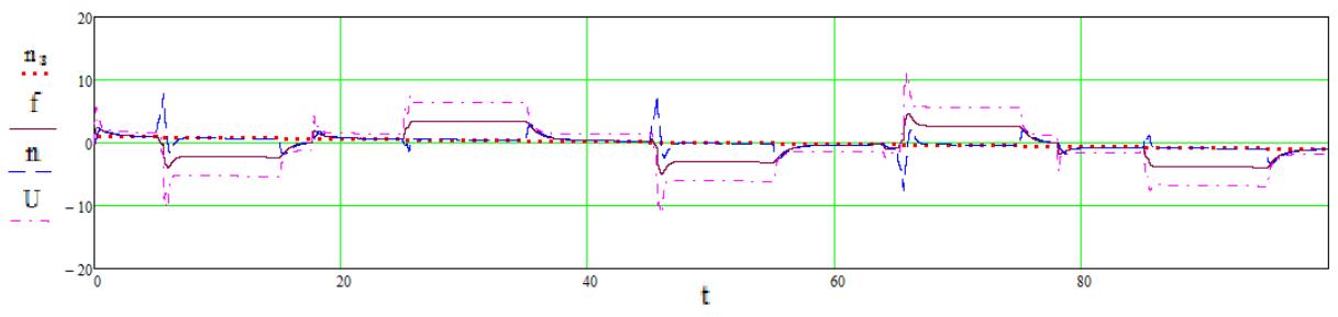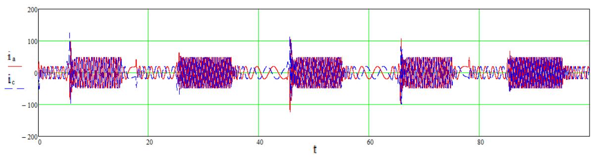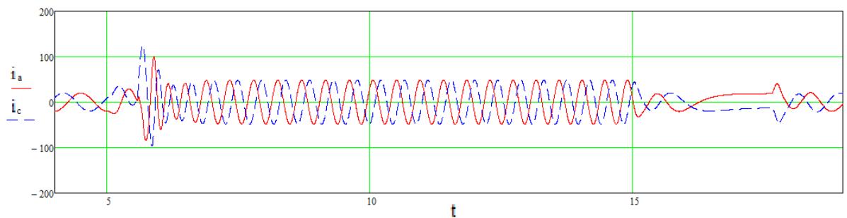 Fig. 4 The modes of operation of the electric drive described here were carefully studied at the Zaporizhzhya Electric Apparatus Plant, including on a crane electric drive with a 20 kW induction motor with an EKT4D-100 frequency converter at different speeds of moving loads up and down, especially at speeds close to zero, and were confirmed by mathematical modeling. ## II. CONCLUSIONS The independence of the electromagnetic torque of the motor from the change of internal resistances allows the asynchronous electric drive with reactive power control to have practically inertialess regulation and inertialess reverse, which is determined by pulse-width modulation of the FC voltage. Such regulation can occur both with large changes in control signals and when the electric drive is operating at a frequency close to zero, including when applying a braking mechanical torque that reduces the frequency to ensure the necessary rotor slippage. To increase the accuracy of the adjustment, the time count when determining the reactive power at low frequencies can be made from the last transition through the zero of the FC output voltage. In the interval of positive and negative frequencies close to zero, in which the error of determining the reactive power is significant, the reactive power is equated to its last value at one or another boundary of the interval. Such properties make it possible to supply an asynchronous electric drive with reactive power control instead of more expensive and less reliable direct current electric drives.

Generating HTML Viewer...