## I. INTRODUCTION Biologists, epidemiologists, economists, and mathematicians have been trying to work together for a long time. In the twenties of the last century, articles by S. N. Berstein appeared, the first of which was "On the application of mathematics to biology" ("Science in Ukraine", 1922, issue 1, p. 14). His next work in 1924 is called "The solution of a mathematical problem related to the theory of heredity". In the future, the genetic theme can be traced in the work of A. S. Serebrovsky (Reports of the USSR Academy of Sciences, 1934, 2, 33) with the unusual-sounding title "On the properties of Mendelistic equalities" and the article by V. I. Glivenko "Mendeleev algebra"(Reports of the USSR Academy of Sciences, 1936,13, 371). This topic was further developed in Europe, for example, Etherington, 1939-1941; Reiersol, 1962; Holgate, 1967-1968. The fate of the remarkable work of A. N. Kolmogorov, I. G. Petrovsky, N. S. is instructive. Piskunov "Study of the diffusion equation connected with an increase in the amount of matter and its application to a biological problem" (Bulletin of Moscow State University, 1937, 1, issue 6, 1-26). It investigated the displacement of an unstable genotype by a stable one. The work has had many imitations in other areas of mathematical natural science. It continued to be studied and quoted even at a time when even mentioning the gene was impossible, which was greatly facilitated by the successful title of the work. It is characteristic of mathematics that the formation of new directions often arises on the basis of new tasks. In particular, all classical analysis arose on the basis of problems of physics, mechanics and geometry. However, later it turned out that the scope of mathematical analysis is much wider. Quite a lot of problems related to chemistry or technology, to various branches of engineering and natural science, including problems of biology and even economics, are solved by methods of mathematical analysis. However, to solve a number of problems in the field of biology, epidemiology of economics, technology, having a cybernetic nature, i.e. related to information flows and management, the methods of classical analysis are not applicable. Tasks of this nature stimulated the development of new branches of mathematics, such as information theory, the doctrine of control systems, as well as automata theory, game theory, various sections of mathematical programming, etc. A common feature of these new areas of mathematics is discreteness. And apparently, this has a deep meaning. The fact is that physics, mechanics and other sciences leading to the formulation of problems of classical analysis are characterized by the expedient use of continuous models of the phenomena under study. In fact, the direct object of mathematical study is continuous media, continuous trajectories, continuous physical fields, etc. At the same time, biology, epidemiology or economics are characterized by the structuring of the object under study. Discrete organelles with a very diverse well-defined functioning are distinguished in the cell. Moreover, the processes of vital activity of the cell consist of the functioning of these organelles. The organism is built from various organ systems, those from individual organs, etc. A somewhat complex economic system is also built from relatively autonomous parts that interact with each other in a very specific way. All this leads to the need to take into account the various elements of the system, specific and sometimes strictly individual interactions between them, as well as taking into account the restructuring of the system as a whole in the process of its functioning. All this is difficult to describe by the methods of classical analysis and leads to the formation of completely new formulations of questions, and therefore new chapters of mathematics. Apparently, somewhat hyperbolizing, we can say that if physics in a broad sense is organically connected with continuous mathematics, then biology, in particular epidemiology in a broad sense, is just as organically connected with discrete mathematics. Based on this, in our work we propose a discrete model for describing the disease of sexually transmitted viral diseases. The spread of sexually transmitted diseases, such as chlamydia, syphilis, gonorrhea (Neisseria gonorrhoeae) and of course the most urgent disease is AIDS, is a very serious health problem in both developed and developing countries. There are more than a million cases of sexually transmitted infections every day. Most of them are asymptomatic. According to statistics from the World Health Organization (WHO), 374 million new cases of infection with one of the four sexually transmitted infections, such as chlamydia, syphilis, gonorrhea or trichoniasis occur every year. For example, in 2016, 376 million cases of infection with one of the four sexually transmitted infections - chlamydia (127 million), gonorrhea (87 million), syphilis (6.3 million) or trichomoniasis (156 million). In 2018, the United States became the record-breaking country for the number of sexually transmitted diseases. There are about 2.5 million people in our country who have fallen ill with these diseases. This number of cases is constantly growing. The most harmless diagnosis was chlamydia. 1.7 million Americans suffer from chlamydia, most of them are women from 15 to 24 years old. At the moment, about 45 percent of women in this age category are infected with chlamydia. Generally speaking, the problem is much more serious than it seems at first glance. Doctors say that the treatment of sexually transmitted diseases is necessary. Today there is a virus super-gonorrhea, resistant to the strongest antibiotics. Because of such viruses, the world can return to the Middle Ages, when millions of people died from such diseases. Of course, we can say that there is no such level of diagnosis in third world countries, so cases of sexually transmitted infections are simply not taken into account. As we can see, research in this area does not miss its relevance opportunity. Models considering sexually transmitted diseases are given in the monograph [1]. A simple epidemiological SI model is considered here, since the cure of, for example, gonorrhea does not lead to the development of immunity, therefore, a person eliminated for treatment becomes susceptible after recovery. Basically, many papers consider continuous dynamical systems described by differential equations. In this paper, we will consider the discrete case of these models, which are fundamentally different from the models considered earlier. We will consider discrete dynamic Lotka-Volterra systems operating in a two-dimensional simplex, and their compositions, since they can be used in modeling the course of sexually transmitted diseases. Let $V: S^{m-1} \to S^{m-1}$ be an arbitrary continuous mapping of the simplex into itself, acting according to the formulas [2] $$ V: x _ {k} ^ {\prime} = x _ {k} \left(1 + \sum_ {i = 1} ^ {m} a _ {k i} x _ {i}\right), k = \overline {{1 , m}}, $$ where $|a_{ki}| \leq 1, a_{ki} = -a_{ik}$ and also $$ S ^ {m - 1} = \left\{x = (x _ {1}, \dots , x _ {m}): x _ {i} \geq 0; \sum_ {i = 1} ^ {m} x _ {i} = 1 \right\} \subset \mathbb {R} ^ {m}. $$ Choose an arbitrary point $x_0 \in S^{m-1}$ and build iterations $x^{(n+1)} = Vx^{(n)}, x(n) -$ the sequence will be called the trajectory of the point $x_0$ when displaying $V$. Since the simplex is compact, the trajectory has at least one limit point. The set of all limit points is denoted by $\omega(x_0) = \{x_0, x_1, \ldots\}' \neq \emptyset$. Theorem 1: ([3]-[4]). Let $A = (a_{ki})$ be a skew-symmetric matrix, in this case $$ P = \{x \in S ^ {m - 1}: A x \geq 0 \} \neq \varnothing , Q = \{x \in S ^ {m - 1}: A x \leq 0 \} \neq \varnothing $$ consist of from fixed points. Let $I = \{1, \dots, m\}$ and for an arbitrary $\alpha \subset I$ we put $$ P_{\alpha} = \{x \in \Gamma_{\alpha} : A_{\alpha} x \geq 0\}, \quad Q_{\alpha} = \{x \in A_{\alpha} : A_{\alpha} x \leq 0\}, $$ where $A_{\alpha}$ is the matrix resulting from the skew-symmetric matrix $A = (a_{ki})$ replacing all $a_{ki}$ with zeros for which $(k,i)\notin \alpha \times \alpha$. Since the narrowing of the Lotka-Volterra mapping to any face of the $\Gamma_{\alpha}$ simplex is also a Lotka-Volterra mapping [4], then it follows from Theorem 1 that the sets $P_{\alpha} \neq \emptyset$ and $Q_{\alpha} \neq \emptyset$ for any $\alpha \subset I$. Let $X = \{x(\alpha): \alpha \subset I\}$ - the set of fixed points. We will say that the fixed points are $x(\alpha)$ and $x(\beta)$ form a pair $(P, Q)$ if there exists a face $\Gamma_{\gamma}$ such that $\gamma = \alpha \cup \beta$ and the following inequalities hold $$ A_{\gamma}x(\alpha)\geq0,A_{\gamma}x(\beta)\leq0. $$ Now the elements of $x(\alpha)$ and $x(\beta)$ we draw on the plane, then if they form a $(P, Q)$ pair, then we connect them with an arc from $x(\alpha)$ to $x(\beta)$. The graph constructed in this way is called a card of fixed points. ## II. METHODS Consider the Lotka-Volterra mappings acting in $S^{m - 1}$, having the form: $$ V _ {1}: x _ {k} ^ {\prime} = x _ {k} \left(1 + \sum_ {i = 1} ^ {m} a _ {k i} x _ {i}\right), k = \overline {{1 , m}}, $$ $$ V _ {2}: x _ {k} ^ {\prime} = x _ {k} \left(1 + \sum_ {i = 1} ^ {m} b _ {k i} x _ {i}\right), k = \overline {{1 , m}}, $$ where $S^{m - 1} = \left\{x = (x_{1},\ldots,x_{m}):x_{i}\geq 0;\sum_{i = 1}^{m}x_{i} = 1\right\} \subset \mathbb{R}^{m}$ Since the Lotka-Volterra mapping is an automorphism of the simplex $S^{m-1}$ into itself, obviously the composition $V_1 \circ V_2$ is also an automorphism, and it is representable as: $$ V _ {1} \circ V _ {2}: x _ {k} ^ {\prime} = x _ {k} \left(1 + f _ {k} \left(x _ {1}, x _ {2}, \dots , x _ {k - 1}, x _ {k + 1}, \dots , x _ {m}\right)\right), k = \overline {{1 , m}} $$ Let us consider a special case of compositions of Lotka-Volterra mappings, for $m = 3$, with coefficients $a_{ki}, b_{ki} = \pm 1$. $$ V _ {1}: \left\{ \begin{array}{l} x _ {1} ^ {\prime} = x _ {1} (1 + x _ {2} + x _ {3}), \\x _ {2} ^ {\prime} = x _ {2} (1 - x _ {1} + x _ {3}), \\x _ {3} ^ {\prime} = x _ {3} (1 - x _ {1} - x _ {2}) \end{array} \right. , \quad V _ {2}: \left\{ \begin{array}{l} x _ {1} ^ {\prime} = x _ {1} (1 + x _ {2} - x _ {3}), \\x _ {2} ^ {\prime} = x _ {2} (1 - x _ {1} - x _ {3}), \\x _ {3} ^ {\prime} = x _ {3} (1 + x _ {1} + x _ {2}) \end{array} \right. \tag {1} $$ here $|a_{ki}| \leq 1, a_{ki} = -a_{ik}, |b_{ki}| \leq 1, b_{ki} = -b_{ik}, \sum_{i=1}^{3} x_i = 1$.  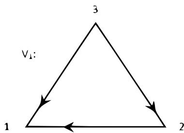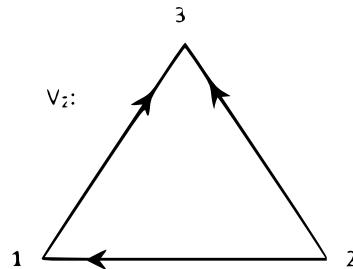 Figure 1. Tournaments corresponding to $V_{1}$ and $V_{2}$. The compositions of these mappings are represented as: $$ V _ {1} \circ V _ {2}: \left\{ \begin{array}{l} x _ {1} ^ {\prime} = x _ {1} \left(1 + x _ {2} - x _ {3}\right) \left[ 1 + x _ {2} \left(1 - x _ {1} - x _ {3}\right) + x _ {3} \left(1 + x _ {1} + x _ {2}\right) \right], \\ x _ {2} ^ {\prime} = x _ {2} \left(1 - x _ {1} - x _ {3}\right) \left[ 1 - x _ {1} \left(1 + x _ {2} - x _ {3}\right) + x _ {3} \left(1 + x _ {1} + x _ {2}\right) \right], \\ x _ {3} ^ {\prime} = x _ {3} \left(1 + x _ {1} + x _ {2}\right) \left[ 1 - x _ {1} \left(1 + x _ {2} - x _ {3}\right) - x _ {2} \left(1 - x _ {1} - x _ {3}\right) \right] \end{array} \right. \tag {2} $$ or $$ V _ {1} \circ V _ {2}: \left\{ \begin{array}{l} x _ {1} ^ {\prime} = - x _ {1} ^ {4} - 4 x _ {1} ^ {3} x _ {2} - 4 x _ {1} ^ {2} x _ {2} ^ {2} + 2 x _ {1} ^ {2} + 4 x _ {1} x _ {2}, \\ x _ {2} ^ {\prime} = - x _ {2} ^ {2} \left(2 x _ {1} ^ {2} + 4 x _ {1} x _ {2} + x _ {2} ^ {2} - 2\right), \\ x _ {3} ^ {\prime} = 1 - x _ {1} ^ {\prime} - x _ {2} ^ {\prime}, \end{array} \right. \tag {3} $$ Since the mapping tournaments $V_{1}$ and $V_{2}$ which are shown in Figure 1 differ in the directions on two edges, i.e. the directions on two edges connecting the vertices $e_{1}$ and $e_{3}$, $e_{2}$ and $e_{3}$ are opposite, and the direction connecting the vertices $e_{1}$ and $e_{2}$ coincide, then in the end we get one more fixed point on two edges $\Gamma_{13}$ and $\Gamma_{23}$. In order to determine the coordinates of these points, we take a narrowing of the composition of these mappings to these edges. For example, to find the location (coordinate) of a point belonging to the edge $\Gamma_{13}$, we take the contraction of the compositional operator on this edge: $$ \left\{ \begin{array}{l} x _ {1} ^ {\prime} = x _ {1} \left(1 - x _ {2}\right) \left(1 + x _ {3} \left(1 + x _ {1}\right)\right), \\ x _ {2} ^ {\prime} = 0, \\ x _ {3} ^ {\prime} = x _ {3} \left(1 + x _ {1}\right) \left(1 - x _ {1} \left(1 - x _ {3}\right)\right), \\ x _ {1} + x _ {3} = 1. \end{array} \right. \tag{2} $$ As a result, we got a point $M_1\left(\frac{\sqrt{5} - 1}{2}; 0; \frac{3 - \sqrt{5}}{2}\right)$. By doing the same for the edge $\Gamma_{23}$, we get $M_2\left(0;\frac{\sqrt{5} - 1}{2};\frac{3 - \sqrt{5}}{2}\right)\in \Gamma_{23}$. We obtained the following theorem: Theorem 2: If the mapping is $V_{1}$ and $V_{2}$ are represented as (1), then their composition (2) has the following fixed points: - the five fixed points belonging to the simplex are the points - $$ e _ {1} (1; 0; 0), e _ {2} (0; 1; 0), e _ {3} (0; 0; 1), $$ and $$ M _ {1} \quad \frac {\sqrt {5} - 1}{2}; 0; \frac {3 - \sqrt {5}}{2} \Big) \in \Gamma_ {1 3}, M _ {2} \quad 0; \frac {\sqrt {5} - 1}{2}; \frac {3 - \sqrt {5}}{2} \Big) \in \Gamma_ {2 3}, $$ - two fixed points outside the simplex belonging to $H$ are the points $N_{1}\left(\frac{-1 - \sqrt{5}}{2};0;\frac{3 + \sqrt{5}}{2}\right)$ $N_{2}\left(0;\frac{-1 - \sqrt{5}}{2};\frac{3 + \sqrt{5}}{2}\right)$, where $H = \{x\in \mathbb{R}^m:\sum_{i = 1}^{m}x_i = 1\}$. Proof 2: The proof of the theorem is obtained by solving system (2) on the narrowing of the corresponding edge. This file may be formatted in both the preprint (the default) and reprint styles; the latter format may be used to mimic final journal output. Either format may be used for submission purposes. Hence, it is essential that authors check that their manuscripts format acceptably under preprint. Manuscripts submitted to AIP that do not format correctly under the preprint option may be delayed in both the editorial and production processes. As a result, the card of fixed points of composition (2) looks like 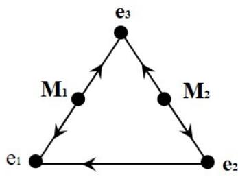 Figure 2: Card of fixed points of composition $V_{1} \circ V_{2}$. Now the main task is to study the nature of the fixed points found. To do this, consider the Jacobi matrix of composition (2). $$ J (V _ {1} \circ V _ {2}) = \left( \begin{array}{c c c} a _ {1 1} & a _ {1 2} & a _ {1 3} \\a _ {2 1} & a _ {2 2} & a _ {2 3} \\a _ {3 1} & a _ {3 2} & a _ {3 3} \end{array} \right), $$ where the coefficients of the matrix have the following form: $$ a _ {1 1} = x _ {1} \left(x _ {2} - x _ {3} + 1\right) \left(x _ {3} - x _ {2}\right) + \left(x _ {2} - x _ {3} + 1\right) \left(x _ {2} \left(- x _ {1} - x _ {3} + 1\right) + x _ {3} \left(x _ {1} + x _ {2} + 1\right) + 1, \right. $$ $$ a _ {1 2} = x _ {1} \left(1 - x _ {1}\right) \left(x _ {2} - x _ {3} + 1\right) + x _ {1} \left(x _ {2} \left(- x _ {1} - x _ {3} + 1\right) + x _ {3} \left(x _ {1} + x _ {2} + 1\right) + 1, \right. $$ $$ a _ {1 3} = x _ {1} \left(x _ {1} + 1\right) \left(x _ {2} - x _ {3} + 1\right) - x _ {1} \left(x _ {2} \left(- x _ {1} - x _ {3} + 1\right) + x _ {3} \left(x _ {1} + x _ {2} + 1\right) + 1\right), $$ $$ a _ {2 1} = x _ {2} (- x _ {1} - x _ {3} + 1) (- x _ {2} + 2 x _ {3} - 1) - x _ {2} (- x _ {1} (x _ {2} - x _ {3} + 1) + x _ {3} (x _ {1} + x _ {2} + 1) + 1), $$ $$ a _ {2 2} = x _ {2} \left(- x _ {1} - x _ {3} + 1\right) \left(x _ {3} - x _ {1}\right) + \left(- x _ {1} - x _ {3} + 1\right) \left(- x _ {1} \left(x _ {2} - x _ {3} + 1\right) + x _ {3} \left(x _ {1} + x _ {2} + 1\right) + 1\right), $$ $$ a _ {2 3} = x _ {2} \left(2 x _ {1} + x _ {2} + 1\right) \left(- x _ {1} - x _ {3} + 1\right) - x _ {2} \left(- x _ {1} \left(x _ {2} - x _ {3} + 1\right) + x _ {3} \left(x _ {1} + x _ {2} + 1\right) + 1\right), $$ $$ a _ {3 1} = x _ {3} \left(- x _ {2} \left(- x _ {1} - x _ {3} + 1\right) - x _ {1} \left(x _ {2} - x _ {3} + 1\right) + 1\right) + \left(x _ {3} - 1\right) x _ {3} \left(x _ {1} + x _ {2} + 1\right), $$ $$ a_{32} = x_3(-x_2(-x_1 - x_3 + 1) - x_1(x_2 - x_3 + 1) + 1) + (x_3 - 1)x_3(x_1 + x_2 + 1), $$ $$ a_{33} = (x_1 + x_2 + 1)(-x_2(-x_1 - x_3 + 1) - x_1(x_2 - x_3 + 1) + 1) + x_3(x_1 + x_2)(x_1 + x_2 + 1) $$ We will find the eigenvalues of the Jacobi matrix by solving the equation $$ | J (x) - \lambda I | = 0. \tag {3} $$ By the values of the eigenvalues of the Jacobi matrix, we can describe the character of fixed points. To do this, we first introduce definitions concerning the nature of fixed points from \[13\]: Definition 1: A fixed point is called attracting (an attractor), if the spectrum of the Jacobian, that is, solutions of equation (3) have absolute values less than one. Definition 2: A fixed point is called repulsive (a repeller), if the spectrum of the Jacobian, i.e. solutions of equation (3) have absolute values greater than one. Definition 3: A fixed point is called a saddle point (i.e. it is neither a repeller nor an attractor) if among the solutions of equation (3) there are those having absolute values greater and less than 1. Recall that it follows from the invariance of the simplex that one $\lambda$ is equal to one, which we exclude from consideration, since in the simplex $\sum_{i=1}^{m} x_i = 1$. As a result, we obtained a general form for the eigenvalues of the Jacobi matrix for system (2): $$ \lambda_ {1} = 1, $$ $$ \lambda_ {2} = 2 x _ {1} ^ {2} x _ {2} - 2 x _ {1} ^ {2} x _ {3} + x _ {1} ^ {2} - 2 x _ {1} x _ {2} ^ {2} + 4 x _ {1} x _ {2} x _ {3} - 4 x _ {1} x _ {2} - 2 x _ {1} x _ {3} ^ {2} + 2 x _ {1} x _ {3} - 2 x _ {1} + x _ {2} ^ {2} + 2 x _ {2} - x _ {3} ^ {2} + 1, $$ $$ \lambda_ {3} = 2 x _ {1} ^ {2} x _ {3} - x _ {1} ^ {2} + 4 x _ {1} x _ {2} x _ {3} - 2 x _ {1} x _ {2} - 2 x _ {1} x _ {3} ^ {2} + 4 x _ {1} x _ {3} + 2 x _ {2} ^ {2} x _ {3} - x _ {2} ^ {2} - 2 x _ {2} x _ {3} ^ {2} + 4 x _ {2} x _ {3} - x _ {3} ^ {2} + 1. $$ Now we calculate the eigenvalues for (each of the fixed) points: $$ e _ {1} (1; 0; 0), \lambda_ {1} = 1, \lambda_ {2} = 0, \lambda_ {3} = 0, e _ {2} (0; 1; 0), \lambda_ {1} = 1, \lambda_ {2} = 4, \lambda_ {3} = 0, $$ $$ e _ {3} (0; 0; 1), \lambda_ {1} = 1, \lambda_ {2} = 0, \lambda_ {3} = 0, $$ $$ M _ {1} \quad \left. \frac {\sqrt {5} - 1}{2}; 0; \frac {3 - \sqrt {5}}{2}\right), \lambda_ {1} = 1, \lambda_ {2} = 0, \lambda_ {3} = 6 - 2 \sqrt {5}, $$ $$ M _ {2} \quad 0; \frac {\sqrt {5} - 1}{2}; \frac {3 - \sqrt {5}}{2} \Bigg), \lambda_ {1} = 1, \lambda_ {2} = 2 \sqrt {5} - 1, \lambda_ {3} = 6 - 2 \sqrt {5}. $$ $$ N _ {1} \quad \left. \frac {- 1 - \sqrt {5}}{2}; 0; \frac {3 + \sqrt {5}}{2}\right), \lambda_ {1} = 1, \lambda_ {2} = 0, \lambda_ {3} = 2 (3 + \sqrt {5}), $$ $$ N _ {2} \quad 0; \frac {- 1 - \sqrt {5}}{2}; \frac {3 + \sqrt {5}}{2}) , \lambda_ {1} = 1, \lambda_ {2} = - 2 (1 + \sqrt {5}), \lambda_ {3} = 2 (3 + \sqrt {5}). $$ As a result, we get the following corollary: Corollary 1: The fixed points defined by Theorem 2 are - $$ \begin{array}{l} - e _ {1}, e _ {3} - \text{attracting}, \\- M _ {2}, N _ {2} - \text{repelling ,} \\- \text{points} e _ {2}, M _ {1}, N _ {1} - \text{saddlefixedpoints}. \\\end{array} $$ Now we are interested in the dynamics of the trajectories of the composition $V_{1} \circ V_{2}$. To do this, we use Theorem 1, i.e. for operator (2), to find the sets $P$ and $Q$, we solve the inequalities from this theorem. To begin with, according to Theorem 1, we find the set $P$: $$ \left\{ \begin{array}{l} x _ {2} ^ {2} \left(1 + x _ {2}\right) + x _ {3} \left(2 - x _ {3}\right) \left(1 - x _ {3}\right) + x _ {2} x _ {3} \left(2 - x _ {2} - x _ {3}\right) + x _ {2} - x _ {3} \geq 0, \\ x _ {1} \left(2 - x _ {1} - 2 x _ {3}\right) \left(x _ {1} - 1\right) + x _ {3} \left(2 - x _ {3}\right) \left(1 - x _ {3}\right) - x _ {1} x _ {3} \left(x _ {1} + x _ {3}\right) - x _ {1} - x _ {3} \geq 0, \\ - x _ {1} \left(x _ {1} + 2 x _ {2}\right) \left(1 + x _ {1}\right) - x _ {2} ^ {2} \left(1 + x _ {2}\right) - x _ {1} x _ {2} \left(x _ {1} + 3 x _ {2}\right) + x _ {1} + x _ {2} \geq 0 \end{array} \right. \tag {4} $$ Then, outside the simplex, the set $P$ $$ P = \left\{ \begin{array}{l} \left\{x _ {1} \approx - 3. 5 5 5 1 2, 3. 5 5 5 1 2 \leq x _ {2} \leq 4. 1 7 3 1 6, x _ {3} = 4. 5 5 5 1 2 - x _ {2}\right\}, \\ \left\{x _ {1} \approx - 3. 5 5 5 1 2, x _ {2} \leq - 0. 0 4 1 8 8 4 6, x _ {3} \approx 4. 5 5 5 1 2 - x _ {2}\right\}, \\ \left\{x _ {1} \approx - 1. 2 9 8 9 8, 1. 2 9 8 9 8 \leq x _ {2} \leq 1. 9 1 7 0 1, x _ {3} \approx 2. 2 9 8 9 8 - x _ {2}\right\}, \\ \left\{x _ {1} \approx - 1. 2 9 8 9 8, x _ {2} \leq - 0. 3 1 9 0 5 3, x _ {3} \approx 2. 2 9 8 9 8 - x _ {2}\right\}, \\ \left\{x _ {1} \approx - 3. 5 5 5 1 2, x _ {2} \approx 1. 9 3 7 0 9, x _ {3} \approx 2. 6 1 8 0 3\right\}, \\ \left\{- 3. 5 5 5 1 2 < x _ {1} < - 1. 2 9 8 9 8, - x _ {1} \leq x _ {2} \leq 0. 5 (1. 2 3 6 0 7 - 2 x _ {1}), x _ {3} = - x _ {1} - x _ {2} + 1\right\}. \end{array} \right. $$ inside the simplex, the set $P$ is a point $M_2\left(0;\frac{\sqrt{5} - 1}{2};\frac{3 - \sqrt{5}}{2}\right)$. Now also, according to Theorem 1, we define the set $Q$ by solving the system $$ \left\{ \begin{array}{l} x _ {2} ^ {2} (1 + x _ {2}) + x _ {3} (2 - x _ {3}) (1 - x _ {3}) + x _ {2} x _ {3} (2 - x _ {2} - x _ {3}) + x _ {2} - x _ {3} \leq 0, \\ x _ {1} (2 - x _ {1} - 2 x _ {3}) (x _ {1} - 1) + x _ {3} (2 - x _ {3}) (1 - x _ {3}) - x _ {1} x _ {3} (x _ {1} + x _ {3}) - x _ {1} - x _ {3} \leq 0, \\ - x _ {1} (x _ {1} + 2 x _ {2}) (1 + x _ {1}) - x _ {2} ^ {2} (1 + x _ {2}) - x _ {1} x _ {2} (x _ {1} + 3 x _ {2}) + x _ {1} + x _ {2} \leq 0 \end{array} \right. \tag {5} $$ $$ Q = \left\{ \begin{array}{l} \left\{x _ {1} \approx 0, 618034, x _ {2} \geq 1, x _ {3} \approx 0, 5 (0, 763932 - 2 x _ {2}) \right\}, \\ \left\{x _ {1} \approx 0, 618034, -2.23607 \leq x _ {2} \leq -0.618034, x _ {3} \approx 0.5 (0.763932 - 2 x _ {2}) \right\}, \\ \left\{x _ {1} \approx -1.29898, -0.319053 \leq x _ {2} \leq 0.643377, x _ {3} \approx 2.29898 - 2 x _ {2} \right\}, \\ \left\{x _ {1} \approx -3.55512, x _ {2} \approx 1.93709, x _ {3} \approx 2.61803 \right\} \end{array} \right. 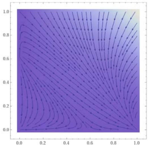$$ inside the simplex, the set $Q$ is this point $M_{1}\left(\frac{\sqrt{5} - 1}{2};0;\frac{3 - \sqrt{5}}{2}\right),e_{1}(1;0;0),e_{3}(0;0;1)$ Now we present a phase portrait of the dynamics of the trajectories of each component of the composition (2). Consider the first of them $x_1' = -x_1^4 - 4x_1^3 x_2 - 4x_1^2 x_2^2 + 2x_1^2 + 4x_1x_2$. Since in this case the first component has the form $x_{1} = f(x_{1},x_{2})$ and for the convenience of visually seeing the phase portrait, we will rewrite this equation as $x_{1}^{4} + 4x_{1}^{3}x_{2} + 4x_{1}^{2}x_{2}^{2} - 2x_{1}^{2} - 4x_{1}x_{2} + x_{1} = 0$. Then the phase portrait of the dynamics of the first component of the system (2) looks like this: 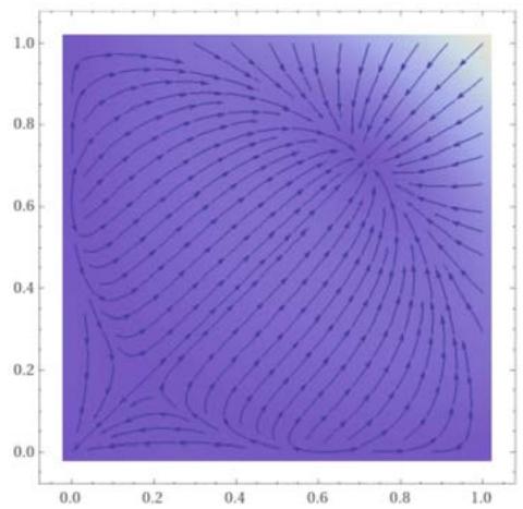 Figure 3: Phase portrait of the dynamics of the first component Now let's move on to the second component. This component is expressed as: $x_2' = -x_2^2 (2x_1^2 + 4x_1x_2 + x_2^2 - 2)$. This component in this case is expressed as $x_2 = f(x_1, x_2)$, then we get the following function, as well as its phase portrait: $-x_2^2 (-2 + 2x_1^2 + 4x_1x_2 + x_2^2) - x_2 = 0$. 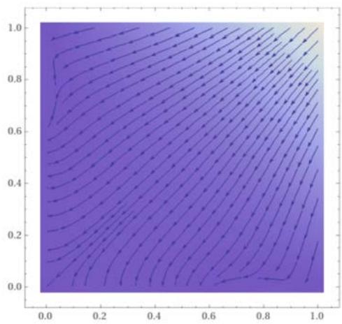 Figure 4: Phase portrait of the dynamics of the second component To see the phase portrait of the third component, use the equality $x_{1} + x_{2} + x_{3} = 1 \Rightarrow x_{3}' = 1 - x_{1}' - x_{2}'$. So the phase portrait of the third component looks like this:  Figure 5: Phase portrait of the dynamics of the third component, represented as the difference of the first two. To explain the phase portrait of each component, we give a complete picture for the entire simplex $S^2$. 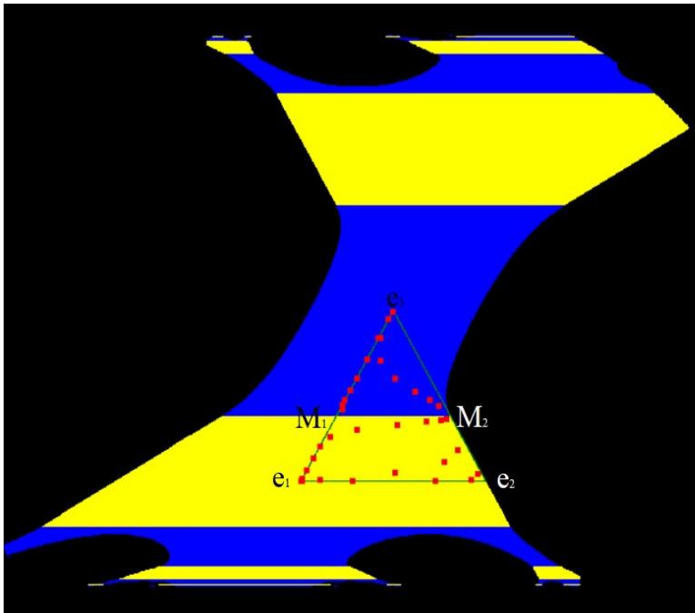 Figure 6: A complete picture of the phase portrait for the entire simplex. To each mapping $V_{1}$ and $V_{2}$ correspond to a transitive tournament (see Fig.1.) and the composition of these maps (2) divides the simplex into two parts. In Figure 6, the yellow color divides the area of the simplex in which all the trajectories of internal points are attracted to the vertex $e_1(1;0;0)$. We can see this flow of trajectories in Figure 3 and Figure 4. These phase portraits show the dynamics of the trajectories of the internal points of the simplex merging into the vertex $e_1(1;0;0)$. And the blue color divides that part of the simplex, the trajectory of the inner points, which are attracted to $e_3(0;0;1)$. The phase portrait of the trajectories of these points is shown in Figure 5. ## III. CONCLUSION Sexually transmitted diseases (e.g. AIDS) have spread in almost all countries of the world. For example, it has been estimated that in some regions of Central Africa up to twenty percent of the population is infected with the human immunodeficiency virus (HIV), and that in the Bronx in New York 13 percent of men and 7 percent of women aged 25-40 years are HIV-infected [18]. To prevent the further spread of these epidemics, it is important to understand how these infectious diseases are transmitted. The transmission dynamics are complex. Many biological and sociological factors are involved. One of the main factors determining the spread of STDs is how people choose their sexual partners. Changes in sexual behavior are recorded in almost every survey of homosexuals or bisexuals and injecting drug users over the past decade [18]. These behavioral changes occur as sexually active people become more careful in their sexual activities to avoid contracting STDs such as AIDS. Understanding the consequences of these behavioral changes can help guide educational programs to prevent STD transmission. The proposed model in this paper represents the contact of a population susceptible to infection, where the first mapping $V_{1}$ – defines a certain population (male or female), and the second $V_{2}$ – defines a certain population (male or female). The dynamics of each component of the composition determines the course of the disease (Figure 3,4 and 5), as well as a complete picture of the phase portrait (Figure 6) of the entire composition divided by two colors gives a territorial limitation of the resulting population in contact with susceptible and infected. The full interpretation in the epidemiological vocabulary of this work will be given in the next article.

Generating HTML Viewer...

References

18 Cites in Article
J Murray (2009). Unknown Title.
R Ganikhodzhaev (1993). QUADRATIC STOCHASTIC OPERATORS, LYAPUNOV FUNCTIONS, AND TOURNAMENTS.
R Ganikhodzhaev,M Tadzhieva,D Eshmamatova (2020). Dynamical Properties of Quadratic Homeomorphisms of a Finite-Dimensional Simplex.
R Ganikhodzhaev,D Eshmamatova (2006). Quadratic automorphisms of a simplex and the asymptotic behavior of their trajectories.
F Harary (1969). Graph theory.
Frank Harary,Edgar Palmer (1972). LABELED ENUMERATION.
J Moon (2013). Embedding tournaments in simple tournaments.
F Gantmacher (1959). The theory of matrices.
William Kermack,A Mckendrick (1927). A contribution to the mathematical theory of epidemics.
Dilfuza Eshmamatova,Rasul Ganikhodzhaev (2021). Tournaments of Volterra type transversal operators acting in a simplex Sm−1.
M Tadzhieva,D Eshmamatova,R Ganikhodzhaev (2021). Volterra-type Quadratic Stochastic Operators with a Homogeneous Tournament.
R Ganikhodzhaev (1994). Map of fixed points and Lyapunov functions for one class of discrete dynamical systems.
D Eshmamatova,R Ganikhodzhaev,M Tadzhieva (2022). Dynamics of lotka-volterra quadratic mappings with degenerate skewsymmetric matrix.
Y Murray (2004). On a necessary condition for the ergodicity of quadratic operators defined on a two-dimensional simplex.
S Ulam (1960). A collection of mathematical problems.
V Volterra (1931). Theorie mathematique de la lutte pour la vie.
Rasul Ganikhodzhaev,Farrukh Mukhamedov,Utkir Rozikov (2011). QUADRATIC STOCHASTIC OPERATORS AND PROCESSES: RESULTS AND OPEN PROBLEMS.
D Xiaoan,L Zhang,H Luo,W Rong,X Meng,H Yu,T Xiaodong (2021). Factors associated with risk sexual behaviours of HIV/STDs infection among university students in Henan, China: a cross-sectional study.
Explore published articles in an immersive Augmented Reality environment. Our platform converts research papers into interactive 3D books, allowing readers to view and interact with content using AR and VR compatible devices.
Your published article is automatically converted into a realistic 3D book. Flip through pages and read research papers in a more engaging and interactive format.
Mathematical ecology as a science began to take shape at the beginning of the XX century. Its emergence was facilitated by the works of outstanding mathematicians like Vito Volterra and his contemporaries L. Lotka and V. A. Kostitsin. Further development of mathematical ecology is associated with the names of G.
Our website is actively being updated, and changes may occur frequently. Please clear your browser cache if needed. For feedback or error reporting, please email [email protected]
Thank you for connecting with us. We will respond to you shortly.