## I. INTRODUCTION Dengue fever (DF) is an arthropod-borne viral disease common past three decades. According to WHO, 51-101 million new infections with dengue occur every year in more than a hundred endemic countries [1]. Dengue fever is a severe viral infection with potentially fatal consequences. Dengue fever was originally known as "water poison." The dengue caused by the female Aedes aegypti mosquito is shown in Fig.1 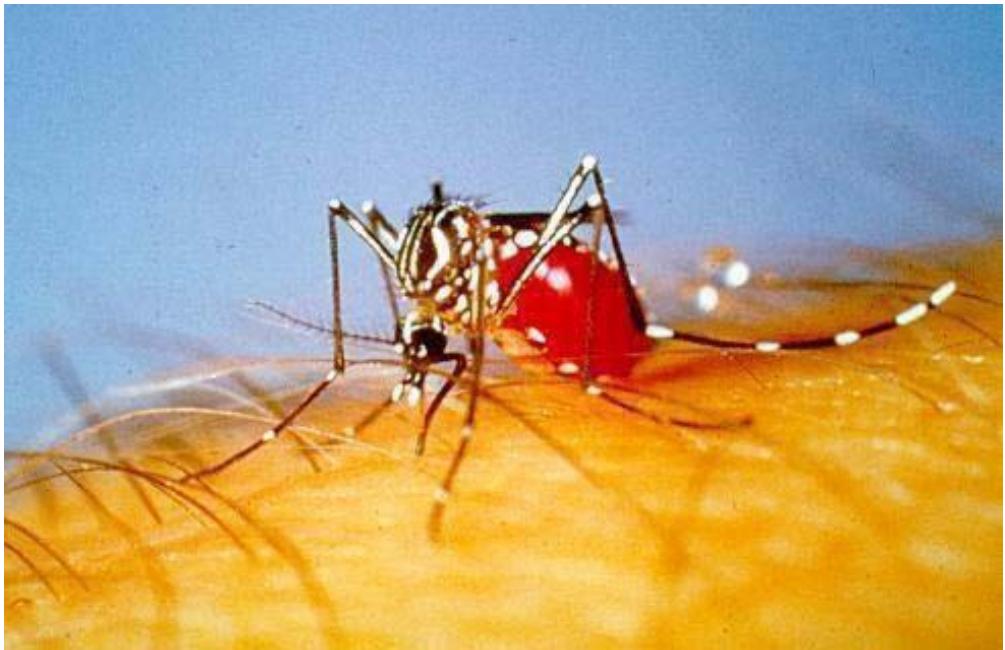 Dengue fever (DF) is an arthropod-borne viral disease Fig. 1: A Female Aedes Aegypti Mosquito In the 1780s, the first clinically recognized epidemics of dengue occurred at the same time in Africa, Asia, and North America. Benjamin Rush was named "break-bone fever" based on the features of arthralgia and myalgia. The dengue epidemic was first reported in Chennai in 1780, the first virologically proven outbreak of dengue fever in India appeared at Calcutta and the East Coast of India in 1963-64. In the 1970s and 1980s, epidemic activity accelerated dramatically, resulting in the widespread of viruses and mosquito vectors and the consequent DENV transmission across the world [2]. The first major DHF epidemic occurred in the Philippines during 1953-1954, continued by a rapid global spread of DF/DHF epidemics. The first major DHF/DSS epidemics in India occurred in 1996, at Delhi and Lucknow, and later extended throughout the country. In India outbreaks of dengue have become more common in many parts. Between 2010 to 2014 incidence of reported cases of dengue was 34.81 per million population. Dengue fever became endemic in Orissa, Uttarakhand, Bihar, Assam, and Jharkhand, in 2010 [3]. ## Dengue Fever: Symptoms and Treatment 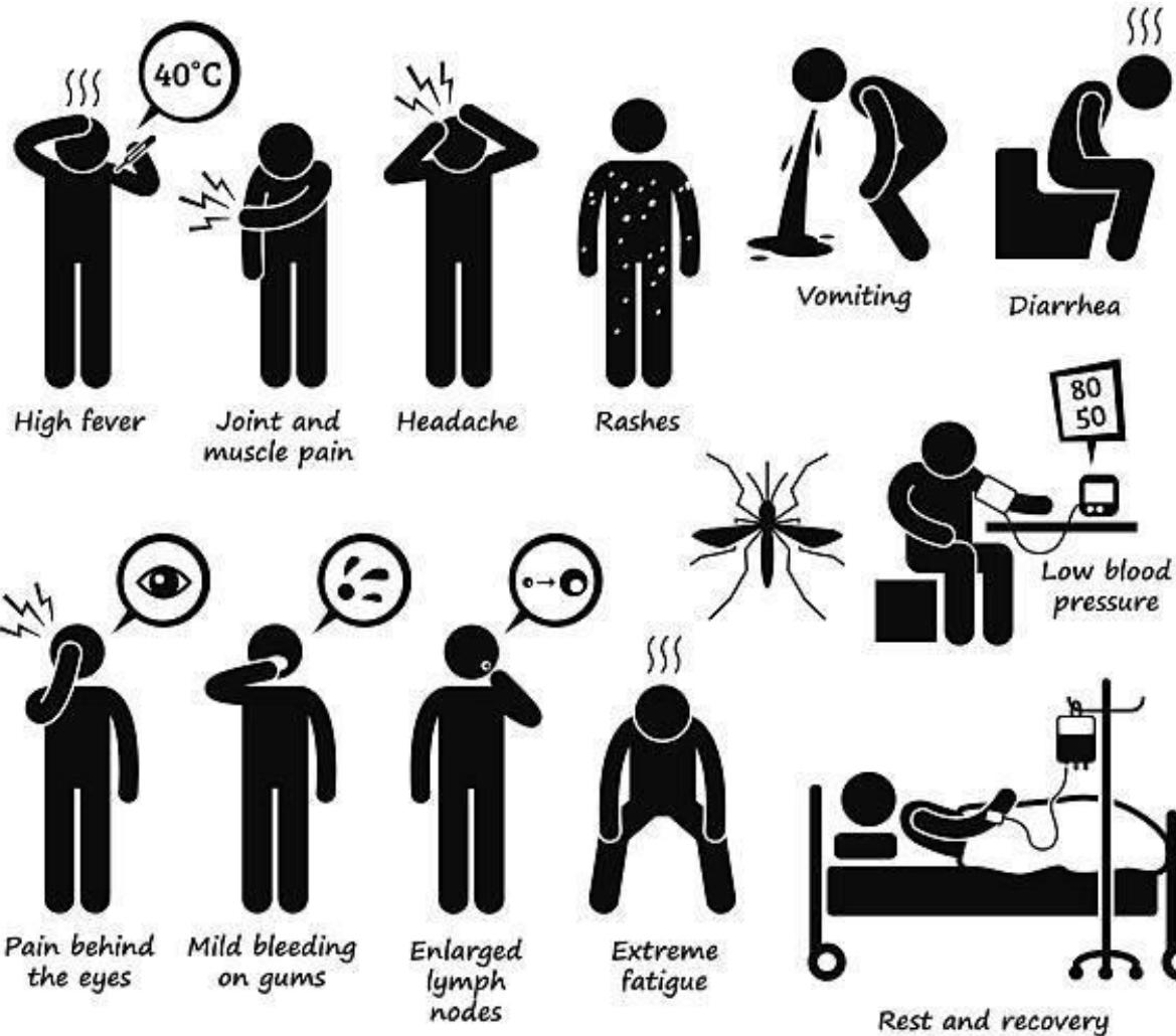 Fig. 2: Pictorial Representation of Dengue Fever Symptoms According to the World Health Organization, Dengue fever is classified into four types: DENV1, DENV2, DENV3, and DENV4. The incubation period is 2 to 7 days [4]. The Dengue symptoms are high fever, joint and muscle pain, headache, vomiting, rashes, pain behind the eyes, diarrhea, etc. The dengue fever symptoms are shown in Fig.2. Different ML algorithms are used for dengue fever classification such as NB classifier, K Nearest Neighbour, Decision Tree, Support Vector Machine, and Neural Networks. The proposed model demonstrates ensemble techniques called bagging, boosting, and stacking. The dengue binary classification is based on Extreme Gradient Boost (XGB), Random Forest by majority voting, and stacking with different metaclassifiers. The techniques are analysed based on different performance measures called accuracy, precision, recall, F measure, and extended analysis done by the ROC curve, precision-recall curve, and AUC. The organization structure is as follows: Section II explains the work carried out and section III describes the proposed methodology. Performance analysis in section V and Section VI concludes the work. ## II. BACKGROUND STUDY Kassaye Yitbarek Yigzaw et al [2] presented a benchmarking platform for the prediction of communicable diseases. Rathi et al [4] studied dengue infection in Rajasthan. The study was based on 100 admitted children and he classified the patients based on their symptoms. Kalayanarooj S [3] demonstrates the clinical appearances of dengue and DHF. Aldallal, A.S [5] explained that data mining techniques are used for the prediction of non-communicable diseases like heart and diabetes. Agrawal et al [7] demonstrated the ensemble approach by using multiple classifiers Ada boost, and a decision tree for the prediction of diabetes. Ghosh et al [10] used multiple classifiers for the sentiment analysis performance assessment. Gupta et al [12] compared different ML approaches for heart disease prediction. Mesafint et al [14] explained ML algorithms for the prediction of HIV/AIDS tests. ## III. PROPOSED METHODOLOGY The ensemble models are Extreme Gradient Boost (XGB), Random Forest (RF) by majority voting, and Stacking, which is based on a combination of heterogeneous classifiers like NB, KNN, and SVM. It is very helpful to consider ensemble techniques [6], for dengue fever diagnosis and prediction. The proposed framework is shown in Fig 3. 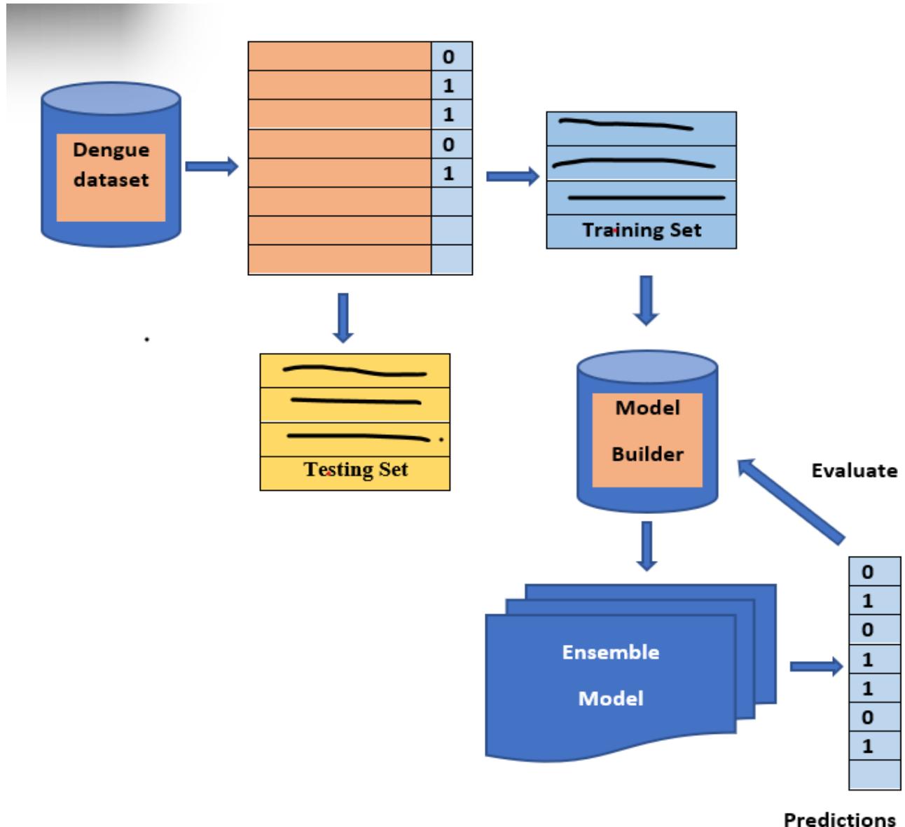 Fig. 3: An Ensemble Frame Work for the Prediction and Evaluation of Dengue Dataset ### a) Data Acquisition and Analysis The main aim of data acquisition and the data pre-processing module is to get the Dengue fever dataset and process them into a suitable form for further analysis. Datasets have features/attributes which will finally distinguish the data into patient sick and healthy. The dataset has thirty-eight features and different data types. The dataset is spitted into an $80\%$ training set and a $20\%$ testing dataset. The pre-processing includes feature selection and missing value imputation [8]. The proposed model combines different classifiers such as Naïve Bayes, K -Nearest Neighbor, and Support vector machine. For each classifier, the output is predicted. Each base classifier is used in the ensemble framework by training data to make it useful for the prediction of dengue. Dataset features and target values are known to each classifier, which in turn can predict whether the disease is present or not. ## i. Description of the Dengue Dataset The patient data is collected from the Department of General Medicine, PESIMSR, Kuppam, Andrapradesh. The patient is diagnosed in the laboratory using the dengue duo card test shown in fig 4. Dataset consists of 18 attributes and one target value. 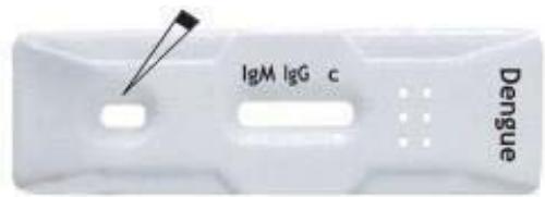 Fig. 4: Diagnosis-Dengue Duo Card Test It consists of 286 instances with 18 attributes and one target. The target consists of dengue patients and Non dengue patients. levels. The numerical value is assigned for each level like 0 for non- dengue patients (NDF), and 1 for Dengue patients (DF). The screenshot of the dataset is shown in Fig.5. 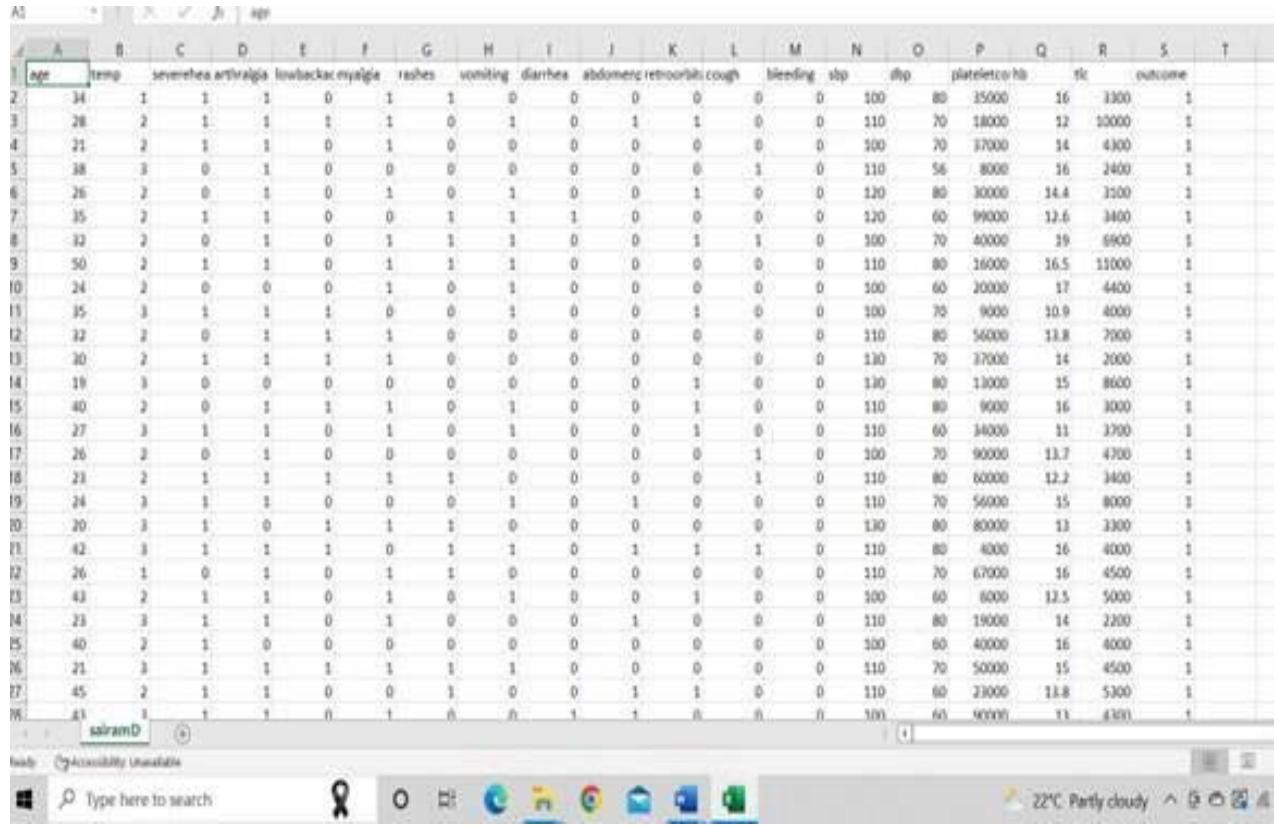 Fig. 5: The screenshot of the dataset The target value consists of 140 cases of dengue infected and 146 non-dengue cases among 286 cases. The distribution is shown in Fig.6 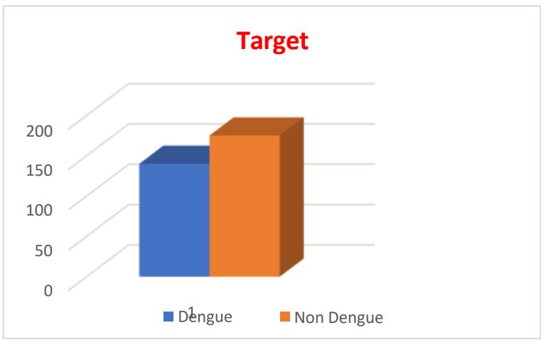 Fig. 6: Distribution of a Target Value The number of patients having each symptom is listed in Table I and corresponding bar charts explain the importance of each feature [9] are shown in fig.7. Among 140 dengue-infected cases all the patients are suffering from fever, 106 headache, 97 and 94 myalgia and arthralgia and 83 low back pain and others. Table 1: Major Clinical Features <table><tr><td>Clinical Feature</td><td>No. of Patients</td></tr><tr><td>Fever</td><td>140</td></tr><tr><td>Headache</td><td>106</td></tr><tr><td>Myalgia</td><td>97</td></tr><tr><td>Arthralgia</td><td>94</td></tr><tr><td>Low Backache</td><td>83</td></tr><tr><td>Retro Orb Pain</td><td>71</td></tr><tr><td>Rashes</td><td>65</td></tr><tr><td>Vomiting</td><td>57</td></tr><tr><td>Pain Abdomen</td><td>41</td></tr><tr><td>Bleeding</td><td>39</td></tr><tr><td>Cough</td><td>30</td></tr><tr><td>Diarrhea</td><td>25</td></tr><tr><td>Sore Throat</td><td>16</td></tr><tr><td>Breathlessness</td><td>6</td></tr><tr><td>Seizures</td><td>5</td></tr></table> 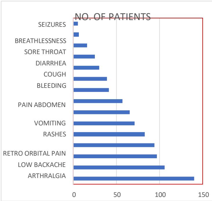 Fig. 7: Bar Chart Representation ### b) Ensemble Methods Ensemble means combining multiple models. This approach gives better performance compared to a single model. Thus, a set of models is used for predictions than a single model [7]. The main challenge is to obtain a base model which gives different kinds of errors. If the ensemble technique of bagging, boosting, and stacking are used for classification, high accuracies can be obtained. Bagging creates a different subset of training data from the sample training dataset & the final output depends on majority voting. e.g., Random Forest. Boosting the creation of sequential models by combining weak learners with strong learners and the finally constructed model has the highest accuracy e.g., XGBOOST and ADA BOOST ## i. Random Forest Algorithm Random forest is a supervised ML algorithm, used for both classification and regression. Random Forest is a bagging ensemble technique and each classifier in the ensemble model is a decision tree. RF constructs decision trees by a random selection of attributes at each node and then determines the split as shown in fig.8. Each tree votes and their majority vote are used for classification and the most popular class is returned. Random Forest Algorithm can handle the data set containing binary, continuous variables as well as categorical variables in case of regression and classification respectively. RF gives better results for classification problems. Random forest is a simple, fast, flexible, and robust model and it can handle missing values [10, 12]. ## ii. XGBoost Boosting is a broadly used and highly effective machine learning algorithm. An end-to-end tree boosting system called XGBoost is widely used by data experts. The important factor is its scalability for better accuracy. The system is ten times faster than existing conventional methods. The scalability of XGBoost is due to several algorithms optimizations. Parallel and distributed computing will make learning faster [15]. 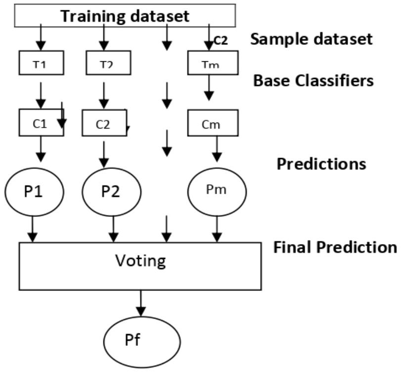 Fig. 8: Random Forest Algorithm Procedure ## iii. Stacking Stacking is an ensemble technique, which uses meta-classifiers to learn, the possible way to combine two or more base ML algorithms predictions. The base or level 0 classifiers consists of different ML algorithms and therefore stacking ensembles are generally heterogeneous classifiers. Level 1 classifiers are used as new features to train a meta classifier. An ensemble stacking procedure is illustrated in fig 9. The meta classifier can be any classifier [13] 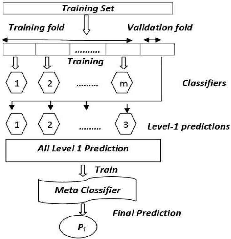 Fig. 9: An Ensemble Stacking Procedure In the stacking algorithm, the base (first-level) classifiers are trained by the same set of the training sample, which is used to prepare the inputs for the meta (second-level) classifier, which may cause overfitting. The stackingCVclassifier uses the cross-validation method. The dataset is split into k folds, and k-1 folds are used to fit the level-1 classifier in k successive rounds. In every iteration, the level-1 classifiers are then applied to the remaining subset. The predictions of the base classifiers are then stacked and which is an input to the level-2 classifier. ## IV. 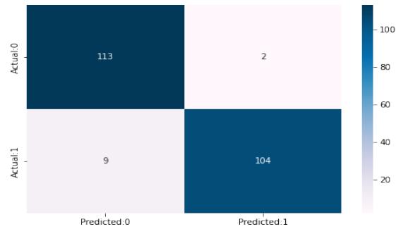PERFORMANCE EVALUATION The clinical dengue fever data set was used to analyse the performance of the ensemble model and to compare it with the other models. The class labels dengue infected (DF) with the dengue not infected (NDF) is replaced with class 1 and class 0 to maintain uniformity [16]. Each dataset is split into training and testing sets. Cross validations of 10-fold are applied. performance measure of each base classifier, as well as the ensemble model, is calculated using a confusion matrix. The base classifiers NB, SVM & KNN are trained first and then they are tested. The proposed research work analysed the performance of the ensemble methods XGB, RF, and Stacking. The metrics are accuracy, recall, precision, and f1-score. The confusion matrix illustrates the actual and predicted classification [15, 17]. The equations (1), (2), (3), and (4), are used to calculate the metrics [17]. Table II: Confusion Matrix <table><tr><td rowspan="2" colspan="2"></td><td colspan="2">Actual</td></tr><tr><td>Dengue Infected</td><td>Non-Dengue Infected</td></tr><tr><td rowspan="2">Predicted</td><td>Dengue Infected</td><td>TP</td><td>FN</td></tr><tr><td>Non-Dengue Infected</td><td>FP</td><td>TN</td></tr></table> $$ A c c u r a c y = \frac{\text{TruePositive} + \text{TrueNegative}}{\text{TruePositive} + \text{TrueNegative} + \text{FalsePositive} + \text{FalseNegative}} \dots \tag{1} $$ $$ \text{Recall} = \frac{\text{TruePositive}}{\text{TruePositive} + \text{FalseNegative}} \dots \tag{2} $$ $$ P r e c i s i o n = \frac{\text{TruePositive}}{\text{TruePositive} + \text{FalsePositive}} \dots \tag{3} $$ $$ F 1 \text{Score} - = \frac{2 * \text{Precision} * \text{Recall}}{\text{Precision} + \text{Recall}} \dots \tag{4} $$ 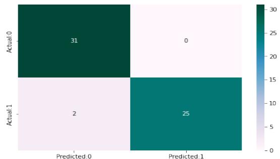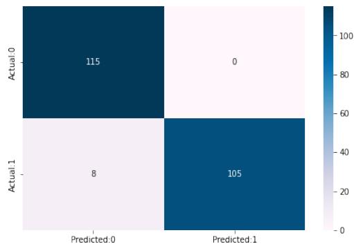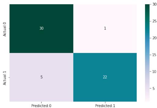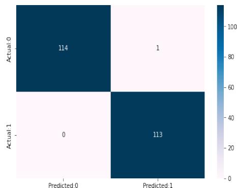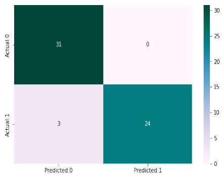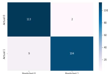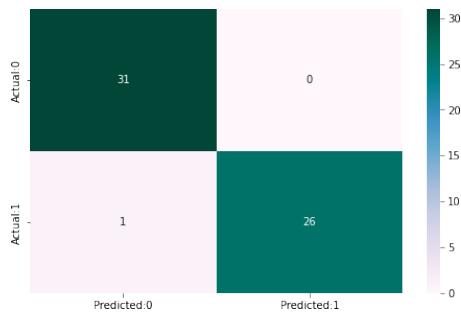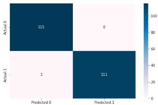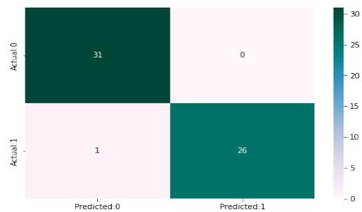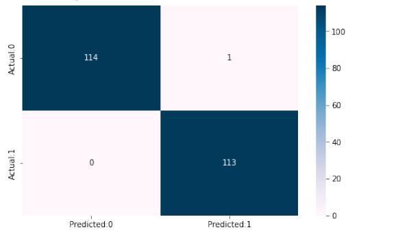The confusion matrix and experimental score of the NB, SVM, KNN, XGB, RF, and Stacking models training dataset and testing dataset are shown in Fig.10.  Training Dataset NB Accuracy of Naive Bayes model: 95.40 <table><tr><td></td><td>precision</td><td>recall</td><td>f1-score</td></tr><tr><td>0</td><td>0.93</td><td>0.98</td><td>0.9</td></tr><tr><td>1</td><td>0.98</td><td>0.92</td><td>0.95</td></tr></table>  Testing dataset NB Accuracy of Naivey bayes: 93.17 <table><tr><td></td><td>precision</td><td>recall</td><td>f1-score</td></tr><tr><td>0</td><td>0.94</td><td>0.98</td><td>0.96</td></tr><tr><td>1</td><td>0.97</td><td>0.93</td><td>0.95</td></tr></table>  KNN Accuracy of K-Neighbors Classifier:96.49 <table><tr><td></td><td>precision</td><td>recall</td><td>f1-score</td></tr><tr><td>0</td><td>0.93</td><td>1.00</td><td>0.97</td></tr><tr><td>1</td><td>1.00</td><td>0.93</td><td>0.96</td></tr></table>  KNN Accuracy of K-Nearest Neighbour: 85.66 <table><tr><td></td><td>precision</td><td>recall</td><td>f1-score</td></tr><tr><td>0</td><td>0.86</td><td>0.97</td><td>0.91</td></tr><tr><td>1</td><td>0.96</td><td>0.81</td><td>0.88</td></tr><tr><td>0</td><td>0.96</td><td>0.98</td><td>0.97</td></tr><tr><td>1</td><td>0.99</td><td>1.00</td><td>1.00</td></tr></table>  SVM Accuracy of Support Vector Classifier: 97.5  SVM Accuracy of Support Vector machine: 89.65 <table><tr><td></td><td>precision</td><td>recall</td><td>f1-score</td></tr><tr><td>0</td><td>0.91</td><td>0.98</td><td>0.94</td></tr><tr><td>1</td><td>0.98</td><td>0.89</td><td>0.93</td></tr></table>  XGB Accuracy of Extreme Gradient Boost:98.57 <table><tr><td></td><td>precision</td><td>recall</td><td>f1-score</td></tr><tr><td>0</td><td>0.99</td><td>0.97</td><td>0.98</td></tr><tr><td>1</td><td>0.97</td><td>0.99</td><td>0.98</td></tr></table>  XGB Accuracy of Extreme gradient Boost:97.80 <table><tr><td></td><td>precision</td><td>recall</td><td>f1-score</td></tr><tr><td>0</td><td>0.97</td><td>0.98</td><td>0.97</td></tr><tr><td>1</td><td>0.98</td><td>0.96</td><td>0.97</td></tr><tr><td>0</td><td>0.98</td><td>1.00</td><td>0.99</td></tr><tr><td>1</td><td>1.00</td><td>0.98</td><td>0.99</td></tr></table>  RF Accuracy of Random Forest: 99.12  RF Accuracy of Random Forest: 94.82 <table><tr><td></td><td>precision</td><td>recall</td><td>f1-score</td></tr><tr><td>0</td><td>0.97</td><td>0.98</td><td>0.97</td></tr><tr><td>1</td><td>0.98</td><td>0.96</td><td>0.97</td></tr></table>  Stacking Accuracy of Stacking CV Classifier:99.56 <table><tr><td>precision</td><td>recall</td><td>f1-score</td><td></td></tr><tr><td>0</td><td>1.00</td><td>0.99</td><td>1.00</td></tr><tr><td>1</td><td>0.99</td><td>1.00</td><td>1.00</td></tr></table> Stacking 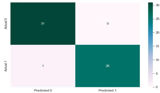 Fig. 10: Confusion Matrix and Experimental Results of Training and Testing Dataset of the Ensemble and Other M Models Accuracy of Stacking CV Classifier: 98.27 <table><tr><td></td><td>precision</td><td>recall</td><td>f1-score</td></tr><tr><td>0</td><td>0.97</td><td>0.99</td><td>0.98</td></tr><tr><td>1</td><td>0.99</td><td>0.96</td><td>0.98</td></tr></table> Table III: Accuracy of Training and Testing Dataset <table><tr><td>Classifiers</td><td>Training Dataset</td><td>Testing Dataset</td></tr><tr><td>NB</td><td>95.40</td><td>93.17</td></tr><tr><td>KNN</td><td>96.49</td><td>85.66</td></tr><tr><td>SVM</td><td>97.51</td><td>89.65</td></tr><tr><td>XGB</td><td>98.57</td><td>97.80</td></tr><tr><td>RF</td><td>99.12</td><td>94.82</td></tr><tr><td>Stacking</td><td>99.56</td><td>98.27</td></tr></table> 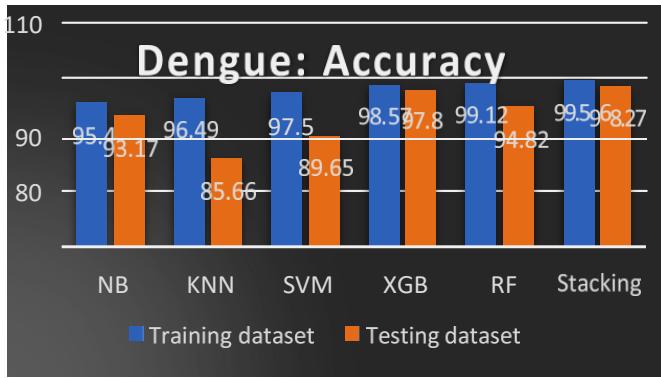 Fig.11: Accuracy Comparison of ML Models The accuracy comparison of the training and testing dataset is shown in Table III and Fig. 11. The ensemble methods XGB, RF, and Stacking give $98.57\%$, $99.12\%$, and $99.56\%$ for the training dataset, whereas $97.80\%$, $94.82\%$ and $98.27\%$ for the testing dataset. We observed better accuracy for ensemble methods. Table IV: Precision, Recall and F1 Score of Training and Testing Dataset <table><tr><td colspan="5">Training dataset</td></tr><tr><td>Classifiers</td><td></td><td>Precision (%)</td><td>Recall (%)</td><td>f1-score (%)</td></tr><tr><td rowspan="2">NB</td><td>NDF</td><td>93</td><td>98</td><td>95</td></tr><tr><td>DF</td><td>98</td><td>92</td><td>95</td></tr><tr><td rowspan="2">KNN</td><td>NDF</td><td>93</td><td>100</td><td>97</td></tr><tr><td>DF</td><td>100</td><td>93</td><td>96</td></tr><tr><td rowspan="2">SVM</td><td>NDF</td><td>96</td><td>98</td><td>97</td></tr><tr><td>DF</td><td>99</td><td>100</td><td>100</td></tr><tr><td rowspan="2">RF</td><td>NDF</td><td>98</td><td>100</td><td>99</td></tr><tr><td>DF</td><td>100</td><td>98</td><td>99</td></tr><tr><td rowspan="2">XGB</td><td>NDF</td><td>99</td><td>97</td><td>98</td></tr><tr><td>DF</td><td>97</td><td>99</td><td>98</td></tr><tr><td rowspan="2">Ensemble Stacking</td><td>NDF</td><td>100</td><td>99</td><td>100</td></tr><tr><td>DF</td><td>99</td><td>100</td><td>100</td></tr></table> <table><tr><td colspan="5">Testing Dataset</td></tr><tr><td>Classifiers</td><td></td><td rowspan="2">Precision (%)</td><td rowspan="2">Recall (%)</td><td rowspan="2">f1-score (%)</td></tr><tr><td></td><td></td></tr><tr><td>NB</td><td>NDF</td><td>94</td><td>98</td><td>96</td></tr><tr><td></td><td>DF</td><td>97</td><td>93</td><td>95</td></tr><tr><td>KNN</td><td>NDF</td><td>86</td><td>97</td><td>91</td></tr><tr><td></td><td>DF</td><td>96</td><td>81</td><td>88</td></tr><tr><td>SVM</td><td>NDF</td><td>91</td><td>98</td><td>94</td></tr><tr><td></td><td>DF</td><td>98</td><td>89</td><td>93</td></tr><tr><td>RF</td><td>NDF</td><td>97</td><td>98</td><td>97</td></tr><tr><td></td><td>DF</td><td>98</td><td>96</td><td>97</td></tr><tr><td>XGB</td><td>NDF</td><td>97</td><td>98</td><td>97</td></tr><tr><td></td><td>DF</td><td>98</td><td>96</td><td>97</td></tr><tr><td>Ensemble</td><td>NDF</td><td>97</td><td>99</td><td>98</td></tr></table> 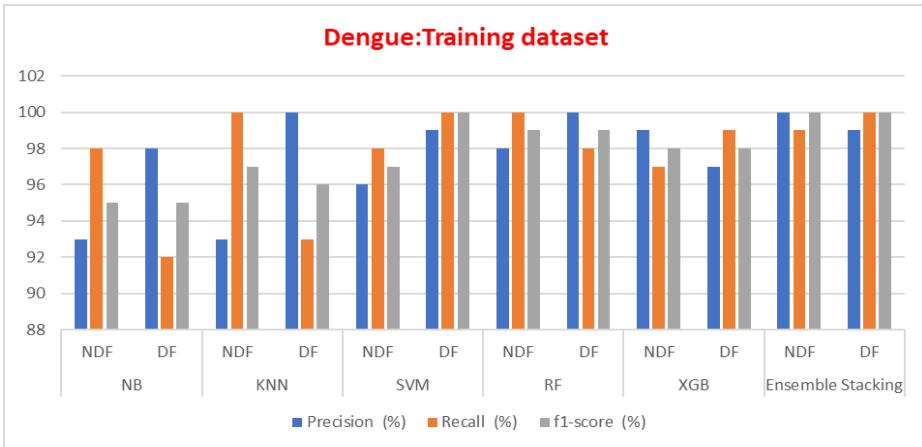 Fig. 12: Training Dataset Precision Recalls and F1 Score Comparison of ML Models 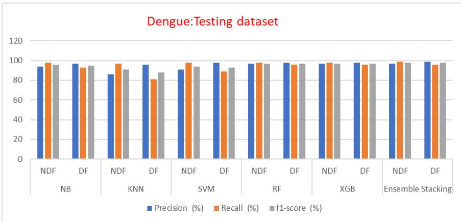 Fig. 13: Testing Dataset Precision, Recall and F1 Score Comparison of ML Models The precision, recall, and f1 score for training and testing datasets are listed in Table IV and a comparison of an ensemble with other methods is shown in fig 12 and 13, which explains the ensemble methods give better performance for unseen data. 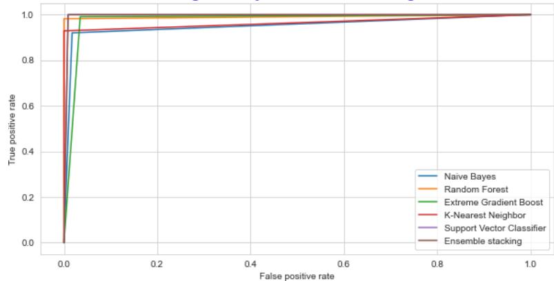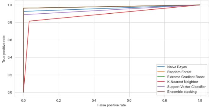The Receiver Operating Characteristic curve and the Precision-Recall curve is a graphical representation of a, by calculating and plotting the false positive rate (FPR) Vs the true positive rate (TPR) and precision Vs recall for each classifier at various threshold values. The precision and recall curve for both training and testing datasets is shown in fig.14 and fig.15 correspondingly the ROC curve is shown in Fig 16 and Fig 17. 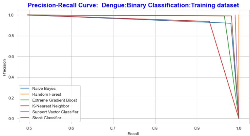 Fig. 14: The Performance Comparison of the Training Dataset by Precision Recall Curve  Fig. 15: The Performance Comparison of the Testing Dataset by Precision Recall Curve  ROC: Dengue Binary Classification-Training Dataset Fig. 16: The Performance Comparison of the Training Dataset by ROC Curve  ROC: Dengue Binary Classification-Testing Dataset Fig. 17: The Performance Comparison of the testing Dataset by ROC Curve The ability of the classifier can be measured by Area Under the (AUC) Curve. It is the summary of the ROC curve. High AUC indicates that the performance of the model is better, wherein differentiating between the positive and negative groups. AUC comparison with other classifiers is listed in TABLE IV. The AUC for the proposed ensemble XGB is $97.14\%$ and $97.81\%$ for random forest $98.14\%$ and $99.14\%$, for stacking $98.14\%$ and $98.68\%$ for testing and Training datasets respectively. As shown in Table III, the AUC values for the datasets lie between 0.97 to 0.99, indicating that the positive class values are correctly distinguished from the negative class values. Table V: Auc Comparison \\begin{table}[htbp]\\centering\\begin{tabular}{I^ccI^c}\\hline\\textbf{Classifier} & \\textbf{Testing Dataset} & \\textbf{Training Dataset} \\\\hline\\text{Auc_Nb} & 0.9629 & 0.9514 \\\\hline\\text{Auc_Knn} & 0.8333 & 0.9342 \\\\hline\\text{Auc_Svc} & 0.9444 & 0.9956 \\\\hline\\text{Auc_Xgb} & 0.9714 & 0.9781 \\\\hline\\text{Auc_Rf} & 0.9814 & 0.9914 \\\\hline\\text{Auc_Scv} & 0.9814 & 0.9868 \\hline\\end{tabular}\\end{table} <table><tr><td>Classifier</td><td>Testing Dataset</td><td>Training Dataset</td></tr><tr><td>Auc_Nb</td><td>0.9629</td><td>0.9514</td></tr><tr><td>Auc_Knn</td><td>0.8333</td><td>0.9342</td></tr><tr><td>Auc_Svc</td><td>0.9444</td><td>0.9956</td></tr><tr><td>Auc_Xgb</td><td>0.9714</td><td>0.9781</td></tr><tr><td>Auc_Rf</td><td>0.9814</td><td>0.9914</td></tr><tr><td>Auc_Scv</td><td>0.9814</td><td>0.9868</td></tr></table> ## V. CONCLUSION The main objective of this research work is to the prediction of dengue fever using ensemble techniques. We used bagging, boosting, and stacking methods for prediction and the end results are compared with the NB, KNN, and SVM models. The experimental results prove that Ensemble techniques are the best models for the prediction of dengue fever. The techniques were analysed using performance metrics. The accuracy for the extended boost, random forest with majority voting, and stacking using metaclassifiers gives better accuracy for both the training and testing datasets compared to other models. The extended analysis was done by using the roc curve and precision-recall curve, which explains the performance of the models. The Area under the curve lies between 0.97 to 0.99. The ensemble models are the better models for the prediction of dengue-infected patients. ### ACKNOWLEDGMENT Our sincere thanks to Dr. Veerapuram Manoj Reddy, Department of General Medicine, PES Medical sciences and Research, Kuppam, Andrapradesh for his support for the collection of dengue data.

Generating HTML Viewer...

References

16 Cites in Article
(2014). Grundy, Fred, (15 May 1905–16 Oct. 1989), Barrister-at-law; Assistant Director-General, World Health Organization, Geneva, 1961–66; retired.
Kassaye Yigzaw,Johan Bellika (2014). A communicable disease prediction benchmarking platform.
S Kalayanarooj (2011). Clinical Manifestations and Management of Dengue/DHF/DSS.
Manisha Rathi,Masand,& Rupesh,Alok Purohit (2015). STUDY OF DENGUE INFECTION IN RURAL RAJASTHAN.
Ammar Aldallal,Amina Al-Moosa (2018). Using Data Mining Techniques to Predict Diabetes and Heart Diseases.
Saba Bashir,Usman Qamar,Hassan Farhan,Khan (2016). IntelliHealth: A medical decision support application using a novel weighted multi-layer classifier ensemble framework.
Julia Miao,Kathleen Miao (2018). Cardiotocographic Diagnosis of Fetal Health based on Multiclass Morphologic Pattern Predictions using Deep Learning Classification.
Monalisa Ghosh,Goutam Sanyal (2018). Performance Assessment of Multiple Classifiers Based on Ensemble Feature Selection Scheme for Sentiment Analysis.
Hanif Heidari,Gerhard Hellstern (2022). Early heart disease prediction using hybrid quantum classification.
Gunjan Gupta,U Adarsh,N V Reddy,& Subba,B Rao,Ashwath (2022). Comparison of various machine learning approaches uses in heart ailments prediction.
K Shaukat,N Masood,S Mehreen,U Azmeen (2015). Dengue Fever Prediction: A Data Mining Problem.
Daniel Mesafint,Manjaiah (2021). Grid search in hyperparameter optimization of machine learning models for prediction of HIV/AIDS test results.
A Tate,U Gavhane,J Pawar,B Rajpurohit,G Deshmukh,Konadala Nynalasetti,Dr Kameswara Rao & Varma,Saradhi (2014). Prediction of Dengue, Diabetes and Swine Flu Using Random Forest Classification Algorithm 16.
H Veena,D Suresh (2021). Comparative Study of Classification algorithms used for the Prediction of Non-communicable diseases.
No ethics committee approval was required for this article type.
Data Availability
Not applicable for this article.
How to Cite This Article
Veena Kumari H M. 2026. \u201cClinical Dengue Data Analysis and Prediction using Multiple Classifiers: An Ensemble Techniques\u201d. Global Journal of Computer Science and Technology - D: Neural & AI GJCST-D Volume 22 (GJCST Volume 22 Issue D2).
Explore published articles in an immersive Augmented Reality environment. Our platform converts research papers into interactive 3D books, allowing readers to view and interact with content using AR and VR compatible devices.
Your published article is automatically converted into a realistic 3D book. Flip through pages and read research papers in a more engaging and interactive format.
Our website is actively being updated, and changes may occur frequently. Please clear your browser cache if needed. For feedback or error reporting, please email [email protected]
Thank you for connecting with us. We will respond to you shortly.