Annotation- In this work, we continue to explore the time inside the plant organism. The beginning of the study of time inside the plant organism is given in [1]. It is shown that inside the plant organism biological time has the character of a vector time field. A dynamic system of two differential equations is constructed, corresponding to this field and corresponding to the whole plant organism (for sunflower). It is shown that such a vector time field divides the plant organism into cellular and subcellular structures. Such a time field has been studied and verified on the basis of data from agrometeorological yearbooks. The calculations of the time axis are made and the phase portrait of the field is obtained.

I. INTRODUCTION

a) Materials and Research Methods

1. Mathematical apparatus

2. Construction of an autonomous system of two differential equations biological vector time field of the plant organism.

3. Study of the autonomous differential system of the vector time field of the plant organism in the Euclidean plane

clause. 3.1 Theoretical results.

clause 3.2. Practical results of calculations of the axis and field of biological time inside the plant organism according to agrometeorological data?? yearbooks Кто за сюво?? оно hyжно??

clause 3.3 Phase portrait of the autonomous dynamic system of the sunflower biological vector time field.

Discussion

II. INTRODUCTION

In this work, we will show that the closed trajectory of the movement of biological time (or simply time) in the plant organism during ontogenesis ensures its division into a cellular structure with subcellular organelles. In the work "On The Closed Trajectory of Movement of Biological Time Inside the Organism of a Plant in Ontogenesis and Everything Secret Becomes Apparent" [1], it was shown and proved that time in a plant organism moves along a closed trajectory. This closed trajectory of time, at its simplest, can be a circle or an ellipse.

Let us give an example: a closed trajectory of the movement of a biological e around the circle. The circle is written in parametric form:

Here $t(j)$ - is a parameter - physical time, varies from small $t_0$ to 1, rel. units, if $t(j)$ is expressed in days $j$, then it is equal to $1/t_E$, $t_E$ — the, where is of the entire ontogenesis, days; $T_F(j)$ — normalized value of the duration biological time corresponding to the process of photosynthesis, rel. un.; $T_R(j)$ — normalized value of biological time corresponding to the process of respiration, rel.un.; $j$ — is the number of the day of the billing period. Day $j$ changes from a small value, corresponding to the "plant shoots" phase, to a certain value of the day, corresponding to the "full maturity of the plant" phase. Number of days from year to year may vary depending on the prevailing agrometeorological conditions.

For the time ellipse of the plant organism, a slightly different parametric equation, see [1].

Thus, the main conclusion is that, as shown in [1], that in a living, growing, plant organism (one-year vegetation period), biological time, or simply time, has a closed nature of movement. This movement is ensured, respectively, by the unchanging movement of our physical time.

Biological time, or simply time, we can explore with the help of mathematical apparatus, and material processes observed in Nature, in the plant organism. Time is not material, like matter, but it can influence material processes.

III. MATERIALS AND RESEARCH METHODS

a) Mathematical apparatus

In the beginning, it is necessary to acquaint you with the necessary mathematical apparatus. This mathematical apparatus is well described in the work of Ac. Pontryagina L.S. together with Ac. Andronov A.A. "Rough Systems" [2], in 1937. This is a system of two autonomous differential equations. In a later book by Bautin N.N. and Leontovich E.A. [3], 1990, methods are presented that allow solving a system of autonomous differential equations on a computer, see also the work of Reznichenko G.Yu. [4].

In [2], a dynamical system of two equations of the first order:

where $x$ and $y$ are Cartesian coordinates on the plane and where $P(x,y)$ and $Q(x,y)$ are analytic functions for all considered values of the variables $x$ and $y$.

We consider such systems of two differential equations (A) for which there is a "cycle without contact". The system (A) is "coarse" in a given domain $G$ if its conditions are satisfied, in contrast to systems that are not "coarse" [2].

Theorem 1. If the system (A) is rough in the domain $G$, then in the domain $G$ the system (A) can have only such equilibrium states for which the real parts of the roots of the corresponding characteristic equation are nonzero [2].

Theorem II. If the system (A) is rough in the domain $G$, then in the domain $G$ the system (A) can have only such periodic motions for which the characteristic exponent is not equal to zero [2].

Theorem III. If system (A) is rough in $G$, then system (A) in $G$ can have only such separatrices (saddle whiskers) that do not go from saddle to saddle [2].

Obviously, rough systems exist. In more detail signs and theorems of the existence of autonomous dynamical systems (A) are presented in the article [2].

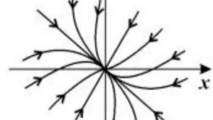
The phase portrait of an autonomous system of two differential equations is considered in the Euclidean plane, which is called the phase plane, and depicts the set of system states (A). The point $M(x,y)$ is called the depicting or representing point. To construct a phase portrait of a dynamic system of two autonomous differential equations (A), the isocline method is used [4]. The main types of trajectories of a dynamic system (A) are shown in Fig. 1.

YcToHBBH y3eI. (1,,AeHCTBHTcJIbHbH OTPHuaTeJIbHb)

HeycToHbH y3eI. $({\lambda }_1,{\lambda }_2$ 1cHCTBHTeJIbHbI H IOIOKHTeJIbHbI)

YcToHnHBnΦOKyc $({\lambda }_1,{\lambda }_2-KOMIIeKCHbI,$ Re

HeycToHnHBnΦOKyC $({\lambda }_1,{\lambda }_2-\kappa \text{OMIIeKCHbI},$ Re

UeHTp. $({\lambda }_1,{\lambda }_2-\mathrm{HCTO}$ MHMBie)

CeIIO. $({\lambda }_1,{\lambda }_2-\text{HCTBHTeHBHbI}$ pa3HbIX 3HaKOB) Fig. 1: The main types of phase trajectories of a dynamical system (A) in Cartesian coordinates, that is, in two-dimensional time space planes

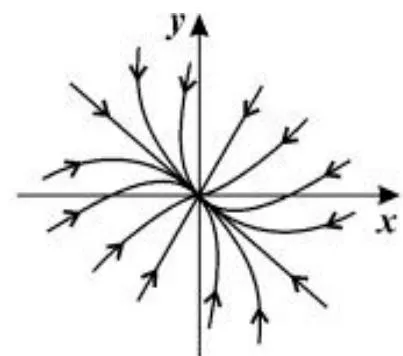
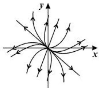
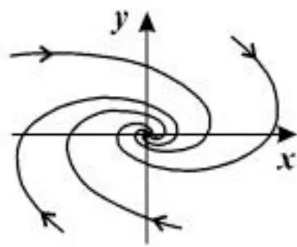
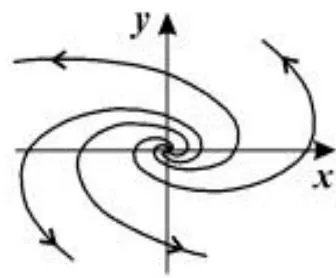
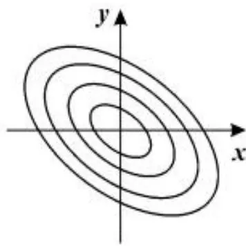
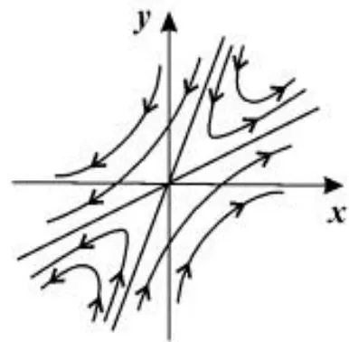
1. Stable node — ${\lambda }_1,{\lambda }_2$ roots of the characteristic equation are real and negative;

2. Unstable node — ${\lambda }_1,{\lambda }_2$ the roots of the characteristic equation are real and positive;

3. Stable focus — ${\lambda }_1,{\lambda }_2$ the roots of the characteristic equation are complex

4. Unstable focus — ${\lambda }_1,{\lambda }_2$ the roots of the characteristic equation are complex ;

5. Center $-{\lambda }_1,{\lambda }_2$ the roots of the characteristic equation are purely imaginary;

6. Saddle — ${\lambda }_1,{\lambda }_2$ roots of the characteristic equation are real and have different signs.

b) Construction of an autonomous system of two differential equations of the biological vector time field of the plant organism

We, in a natural way, will construct an autonomous system of differential equations of a biological vector time field. To do this, we first calculate the vector time axis of the plant organism:

where $d{T}_{opt}$ - is the biological time differential under optimal agrometeorological environmental conditions (Light; Heat; Moisture; Mineral Nutrition), constant, rel. units; $dT(j)$ - environment is the biological time differential under the current agrometeorological environmental conditions, rel. Units; $U(j)$ - environment - the level of tension of environmental factors, depends on the current agrometeorological conditions, rel. units, shows the ratio of ${\mathrm{CO}}_2$ gas exchange of the whole plant organism under current agrometeorological environmental conditions to ${\mathrm{CO}}_2$ gas exchange under optimal agrometeorological environmental conditions of the whole plant organism at the same moment of ontogenesis; $T_0$ - is the initial value of the biological time vector of the plant organism, its length, rel. units; $T(j)$ - is the current value of the biological time vector of the plant organism, its length, rel. Units.

Equation (1) is considered in the time interval from "plant shoots" to "flowering", which corresponds to values from small $T_0$ to 1.

Let us find the integral of equation (1):

where ${[\mathrm{U}(\mathrm{j}{)}_{\text{environment }}]}_{\text{average}}$ - is the average value of the level of tension of the external environment for the period of time from the "shoots" to the current moment of integration - $T(j)$, rel.units.

This integral (2), in a natural way, shows how the length of the biological time vector is summed up in the plant organism. At the same time, the original sum equation [5] was used in the integral:

where $j=1$ - corresponds to the vegetative phase "shoots"; $\mathrm{\Delta }{T}_{opt}$ - is the increase in biological time under optimal agrometeorological environmental conditions for one day of calculation, rel. units; $n$ - respectively, the number of days before flowering.

In the integral (2), it is considered that the division of ontogenesis into parts is one day of calculation. The function of the biological time vector is continuous for the plant organism and changes from day to day.

In the integral (2), the level of intensity of agrometeorological environmental factors $[U(j{)}_{\text{environment}}]$ average - is taken not for a given moment of ontogenesis, but as some average value from the beginning of the integration moment $T_0$ to the current integration moment $T(j)$, rel.units. Then the whole complex of agrometeorological factors of the external environment that influence the rate of biological time flow in a certain interval of integration is taken into account.

Thus, equation (2) expresses the vector axis of biological time in the first half of ontogeny, before the vegetative phase "flowering", in the time interval ${\mathrm{T}}_0\le T(j)\le T$ flowering.

Since the level of intensity of agrometeorological environmental factors $[\mathsf{U}(\mathsf{j}{)}_{\text{environment }}]$ average does not depend on the biological time vector $T(j)$ of the plant organism, this function can be taken out of the integration sign as a constant:

The average value of the intensity level of agrometeorological environmental factors

${[\mathsf{U}(\mathsf{j}{)}_{\text{environment }}]}_{\text{average,}}$ for a certain interval of integration $[T_0;T(j)]$ is found as an integral:

That is, the plant organism, in the process of its life, selects the average value of all environmental factors up to the current moment of ontogenesis.

We introduce the integral(5)into the equation of the integral(2). We will get a double integral, already in a two-dimensional time space. And this double integral is in the Euclidean time plane with its domain of definition${\mathsf{G}}_{\mathsf{FR}}$

two-dimensional time space. And this double integral is in the Euclidean time plane with its domain of definition ${\mathsf{G}}_{\mathsf{FR}}$:

The differential $d{G}_{FR}$ consists of a simple product of two differentials: $d{T}_F$ and $d{T}_R$.

The domain of the $G_{FR}$ of the double integral (6) is a square with its boundary. You can of course also consider a rectangle.

According to [1], in the organism of an annual plant, there is a closed region of integration of the vector biological time field. This is a closed circle or ellipse [1], obtained by Green's formula, the area of this contour is always equal to 1:

where $T(j)$ - is the work of the force field of the total biological time for the entire plant organism for the entire ontogeny, (rel. units of biol. Time) ${}^2$; $V_p$ - is a closed contour, our time circle along which the integration of a closed curvilinear integral of the second kind takes place; $\alpha$ and $\beta$ are dimensionless parameters, they should always equal 1 in their sum, and, they provide a change of a closed circle to a various closed ellipse, depending on their values; $T(j{)}_{Fp}$ - parametric circle equation for time processes of photosynthesis, rel. units; $T(j{)}_{Rp}$ - is the parametric circle equation for temporary

breathing processes, rel. units; $d{T}_{F\rho }$ and $d{T}_{R\rho }$ are the differentials, respectively, of the time processes of photosynthesis and the time processes of respiration of the plant organism; $G_{\rho }$ - is a two-dimensional time domain of integration, located in the plant body, and which is closed, having its own area: the area of the time domain of the plant organism in relative units of time $G_{\rho }(E)=\pi \cdot p^2=1$ [1].

To go from time $T(j)$ to physical time $t(j)$, the following equations are used for time differentials of photosynthesis and respiration processes:

where $t(j)$ - is the physical time, from the phenological phase "shoots" to the phenological phase "flowering", days.

Taking into account equations (8) [1], where it is proved that the movement of biological time goes along a closed trajectory, for further consideration of equation

(6), we need to switch to polar time coordinates, since the time domain $G_p$ is a time circle of radius

$\rho =\sqrt{\frac{1}{\pi }}=0.5642$ [1]. Then the integral (6) can be written in the form:

The region of integration $G_{\rho }$ will be a circle of radius $\rho$. In this case, the polar coordinates have a singular point $\rho =0$. Such a value of $\rho$ cannot exist, since in the seeds of plants there is always some non-zero, structural formation of biological time - a living seed. At the same time, the radius lying in negative values along the $x$ axis is excluded from the region $G_{\rho }$. In our case, $\rho$ can vary within:

for the interval of biological time $[T_0,1]$.

Taking into account (11), the integral (10) takes the form, where we have passed to the iterated integral:

where $\theta$ - is the angle of rotation of the biological time vector, see also my works [5, 6];

To continue the reasoning, we need to consider the transition from the area of integration of the double integral (6) $G_{FR}$ - which is a square, to the area of integration of the double integral (10) $G_{\rho }$ - which is a circle.

Taking into account the fact that our physical time is a vector field, where the time field vector at any point of our three-dimensional space (approximately, not taking into account the influence of gravity) moves in a straight line, and the biological vector time field inside the plant organism is closed $G_{\rho }$ [1], then we have a reflection that is carried out by the plant organism during ontogenesis, in the process of photosynthesis and respiration, and, in general, in the cells of the whole plant during their life:

Then we have another integral equation (10), where in the plant organism, during its life, there is a linear transformation of the vector Euclidean time plane (physical time) into a time vector plane with polar coordinates. Then, in the plant organism, we will have a closed trajectory of biological time. This fact can be represented by an equation, taking into account equations (13) and (14):

where $T_{\rho }(j)$ - is the result of a linear transformation of the Euclidean temporal plane (physical time) into a temporal plane expressed in polar coordinates, thus, we get that

in the plant organism, during its life, the vector biological time moves from the "seed" to "seed".

Consider the integrand of equation (15):

For such a consideration, we use Theorem I. From [2], which says: in the $G_{FR}$ region, system (A) cannot have equilibrium states $x=x_0$, $y=y_0$:

a) for which

b) for which

and Theorem II, which says: in the $G_{FR}$ region, system (A) cannot have periodic motions $x=\phi (t)$, $y=\psi (t)$ [ $\phi (t+\tau )=\phi (t)$; $\psi (t+\tau )=\psi (t)$ ], for which:

Our integrand (16) has a rotating matrix:

where:

and the corresponding determinant.

In this case, we have, according to the condition of Theorem I (20):

In total there are $4!=24$ substitutions of elements A, B, C and D. Depending on this, there will be different differential equations from the matrix (20). Let's provide a finding of one system of two differential equations of a vector temporary biological field of the first order. Then we have, according to equation (A):

where $C_1$ and $C_2$ are integration constants, represent, in our case, a bunch of time field, which can be located in chromosomes, and is a moving element, rel. time $\cdot$ day ${}^{-1}$. Systems of equations (A.1 and A.2) where $C_1$ and $C_2$ are equal to zero are not considered.

Thus, an autonomous differential system of the vector time field was obtained, which is present in the seeds, and later, in the whole plant organism in the process of its growth and development.

c) Study of the Autonomous Differential System of the Vector Time Field of the Plant Organism in the Euclidean Plane

This representation of the time field (A.1 and A.2) immediately determines the structural organization of the field. Such a field is immediately divided into a finite number of connected cells, and each cell has its own sink and source. This representation of the time field corresponds to the cellular theory of the plant organism. Closed trajectories of the time field will determine the oscillatory process in the system of the plant organism. It is well known that light is the first necessary condition for the process of photosynthesis. Therefore, it can be assumed that such an oscillatory process corresponds to electromagnetic oscillations of Photosynthetic Active Radiation - FAR. The fact of mechanical vibrations of the material structure in the leaves of sunflower, corn and sugar beet [7], and for Plasmodium [8] was recorded.

Clause 3.1 Theoretical results

In the work of Ak. Pontryagina L.S. and Ak. Andronova A.A. [2] gives 11 topological types of integral trajectories of a rough dynamical system of motions of differential equations (A). Let's just compare these trajectories with the organization of the plant organism, Table. 1. This table was obtained on the basis of a comparison of the results of [2] and the results of cytological studies presented in [11]. We will not present here the theorems and definitions given in [2]. We will only say that these theorems and definitions are important for the autonomous system of the vector time field (A.1 and A.2) of the plant organism. See also my works [9 and 10].

I. States of equilibrium:	The node (focus)	1	Ribosome
	Saddles	2	Chromatin
II. limit cycles		3	Cell nucleus (control structure)
III. Separatrixes:	Leaving the node (focus) or tending to the node (focus)	4	Mitochondria
	Collapsing from the limit cycle or tending to the limit cycle	5	Chloroplast
	Included in the field Gp	6	Cell wall
IV. Trajectories having as their limit trajectories only nodes (focus) and limit cycles located in the domain Gp	Leaving the node (focus) and tending to the node (focus)	7	Golgi apparatus
	Collapsing from the limit cycle and tending to the limit cycle	8	Plasmodesma
	Leaving the node (focus) and tending to the limit cycle (or vice versa)	9	Lysosome
V. Trajectories entering the domain Gp and not being separatrices:	Aspiring to the node (focus)	10	Vacuole
	Aspiring to the limit cycle	11	Endoplasmic reticulum

Clause 3.2. Practical results of calculations of the axis and field of biological time inside the plant organism according to the data of agrometeorological yearbooks In order to carry out a practical verification of the provisions on biological time outlined in this work, it is first necessary to calculate the vector axis of biological time, in accordance with equation (3), on the integral sum of total increments. After that, it is necessary to determine the moment of violation of the roughness conditions of the autonomous system of the vector time field (A.1 and A.2) of the plant organism and the cardinal points on this time axis.

Let's carry out such a calculation for the sunflower culture, which grew in the Odessa region. Let's define the vegetative phases, "flowering", and then "budding". Calculations of the vegetative phase "full ripening" of sunflower are not given.

According to equation (3), it is considered that for the "seedlings" phase, the biological time vector is equal to $T_0(j)=0.01$ relative time unit day ${}^{-1}$; $\mathrm{\Delta }{T}_{opt}$ - be as 1/65, where 1 is the time interval from the "seedlings" phase to "flowering", relative units, 65 days is the average value of the number of days according to agrometeorological yearbooks for the period 1975-1989 from the phase "seedlings" to the "flowering" phase, and is taken equal to $\mathrm{\Delta }{T}_{opt}=0.02$ relative time unit day ${}^{-1}$. The integral sum (3) was found with a step of 1 day. For the Odessa region, there are 8 agrometeorological stations. Then the average value was found in general for the Odessa region according to the data of these stations. The calculations were carried out on the basis of average ten-day values of environmental factors: "light - FAR", "heat - air temperature", "moisture - reserves of productive moisture in the soil of the 0-100 cm layer".

Also, calculations were made of the violation of the conditions for the roughness of the dynamic system of time in the body of a sunflower plant (A.1 and A.2) and compared with the date of the "budding" phase. Among the three theorems, necessary and sufficient conditions for the existence of a rough system, there is a characteristic exponent $\sigma$ (18), [2]. The value of the characteristic index $\sigma$ cannot be equal to zero $\sigma \ne 0$. In the case of $\sigma =0$, the coarse system (A) and, therefore, (A.1 and A.2) ceases to be coarse and becomes a dynamic system of the first and other degrees of noncoarseness [2]. That is, the system (A) is rough if the separatrices (saddle whiskers) do not go from saddle to saddle, fig. 2.

a

b

C Fig. 2: Separatrices of saddles: a - separatrices go from saddle to saddle, the system (A.1 and A.2) becomes "not rough"; b, c - separatrices do not go from saddle to saddle, the system (A.1 and A.2) is "rough" (according to [3]).

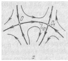
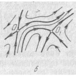
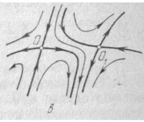
For comparison, the "roughness" of the system of the biological vector time field of the plant organism

(A.1 and A.2) is seen in the example of division in the cell of the aloe root - fig. 3.

or:

With this characteristic exponent, there are two conditions when it is equal to zero:

Condition (29) is satisfied when the biological time vector is orthogonal to physical time. This means that the development of the plant organism is suspended. Suspension of sunflower development can be only if the level of environmental factors drops to biological zero. Which can happen very rarely. Usually the level of environmental factors is high enough to carry out growth and development in the climatic conditions of sunflower growth. At the same time, condition (28) is always fulfilled at the beginning of cell division in the stem meristem for the future basket. Taking into account the fact that the vector of the biological time field has the property of closure and moves in a circle [1], then our condition (28) turns into the following formula:

On the interval of physical time from $T_0$ to 1, which is equivalent to the phase "shoots" to the phase "flowering". Based on these conditions, calculations were carried out for the Odessa region, where the moment of fulfillment of condition (30) was noted. The calculation results are given in Table 2.

Year	Physiological event of sunflower plant
	Phase "budding"		phase "flowering"
		Fact Days from "shoots"	Calculation Days from "shoots"	Fact Days from "shoots"
1975	29	40	64	63
1976	29	43	69	68
1977	34	39	60	66
1978	29	41	58	66
1979	28	34	58	58
1980	31	42	55	66
1981	28	38	60	64
1982	25	40	60	64
1983	28	37	71	66
1984	---	---	---	----
1985	26	32	58	66
1986	30	41	64	66
1987	30	37	69	62
1988	28	40	61	65
1989	27	44	65	65
Сре indianee	29	39	62	65

The average error of the estimated the phase "flowering" date deviates from the actual date by $6.7\mathrm{\%}$.

As can be seen from the data presented in Table. 2, the moment of violation of the "roughness" of the dynamic system of the biological time field (A.1 and A.2) precedes the "budding" phase by an average of 10 days. If we take into account that the "budding" phase is visually fixed during observations of the culture, like a bud that has appeared, then 10 days are just necessary for such visual fixation.

Clause. 3.3 Phase portrait of the autonomous dynamic system of the sunflower biological vector time field

The phase portrait of the vector biological time field system was built using the finite increments method. By setting the increment , we obtain the corresponding increments $\mathrm{\Delta }x$ and $\mathrm{\Delta }y$ from the expressions [4]:

Then the direction of the vector at the point $(x,y)$ will determine the structural organization of the field without an explicit, analytical solution of the system of equations (A) or, which is the same, our system of equations (A.1 and A.2). The construction of a phase portrait allows us to draw conclusions about the nature of the changes in the variables $x,y$ without knowing the analytical solutions of the original system of equations (A.1 and A.2). Moreover, the system (A.1 and A.2) has no explicit solution.

The phase portrait of the system (A.1 and A.2) for two variables $T(j)$ and $\theta (j)$ is shown in fig.

First of all, it should be noted that the dynamic system (A.1 and A.2) divides the domain of existence of the variables $T(j)$ and $\theta (j)$ into a finite number of connected cells - plant cells. At the same time, all topological types of integral trajectories of the vector biological time field of the plant organism are present in the results obtained.

Fig.3 clearly shows the chromatin of the cell. And this chromatin, as the division process proceeds, from the beginning of cell division, to the formation of two new cells, first "rough", then "not rough" - separatrices of saddles go from saddle to saddle - and at the end of cell division, or mitosis, two cells with coarse chromatin. See also

Fig. 4: Phase portrait of the dynamic system of the vector biological time field of the sunflower organism (A.1 and A.2) for two cases: A - the level of tension of environmental factors $U_{sr}=U(j{)}_{\text{environment}}=0.9$ rel.un., this value is accepted for the entire time interval from $T_0$ to 1, or what is the same from the "shoots" phase to the "flowering" phase, or what is the same in the figure - from 0 to 5000; B - tension level of environmental factors $U_{sr}=U(j{)}_{\text{environment}}=0.5$ rel.un., from $T_0$ to 1, or what is the same, you can see in the figure the variable $T(j)$ changes from 0 to 5000, and the variable $\theta (j)$ changes from 0 to 3.5 π, the resolution step is = 54 days·24 hours·60 minutes·60 seconds = 4,665,600 seconds, or, divided by 5000 = 933.12 seconds or 15.552 minutes

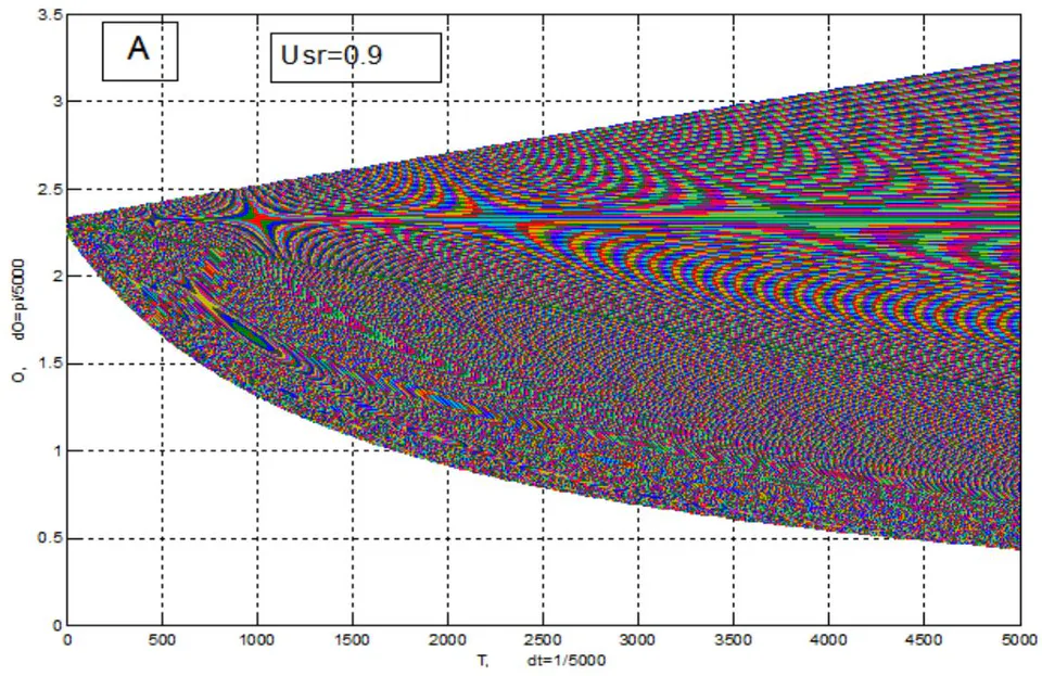
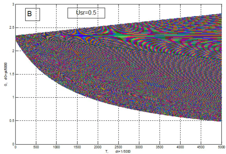
The integral trajectories fill the entire region of the space $G_{\rho }$. Integral trajectories of the vector biological temporal field have all possible directions and permeate the entire domain of definition, which corresponds to the integrity of the plant organism. The integration constants $c_1$ and $c_2$ correspond to the sunflower culture and make up the values: $c_1=0.65$ rel. units biological time and $c_2=0.28$ rel. units biological time and found as a result of a simple study by the substitution method. These constants can be written as: $c_1=\sum _{i=1}^{N_1}{c}_i$ and

$c_2=\sum _{k=1}^{N_2}{c}_k$, where $N_1$ and $N_2$ are numbers that add up to $N_1+N_2$ to double the number of plant chromosomes, that is, time clots.

On fig. 4, for two figures A and B, the entire region $G_{\rho }$ of the vector biological time field is divided by the integral straight line into two sub-regions: upper and lower. The upper sub-region corresponds to the above-ground part of the plant, and the lower sub-region corresponds to the roots. In the upper sub-region there is an integral trajectory (straight line) on which integral trajectories are sequentially arranged according to the saddle type. Moreover, the whiskers of these saddles go from saddle to saddle, which violates the conditions for the roughness of the dynamic system of the vector biological time field, intensive cell division occurs on these trajectories. Thus, these given trajectories correspond to the meristem of the stem, or tissue of the growth cone of the above-ground shoot. The zero points of successive saddles correspond to the moments of the beginning of the laying of leaves, and the last saddle corresponds to the laying of the reproductive organ. The lower subregion corresponding to the roots does not contain saddle trajectories, where the saddle whiskers go from saddle to saddle, which indicates the absence of a "limit cycle" control structure in the roots, which is the control structure of the growth cone of the above-ground shoot. Near the lower boundary of the subdomain corresponding to the roots, in Fig. 4 shows the intensive formation of small cells - root endings.

Depending on the state of environmental factors (Figure 4 - A and Figure 4 - B), the proportion of roots in the whole plant body changes. Thus, under more intense environmental conditions, $U(j{)}_{\text{environment}}=0.5$, the proportion of roots in the plant organism increases. At the same time, the share of the aerial part of the plant organism decreases. Thus, the level of tension of environmental factors determines the growth and development of the plant organism.

IV. DISCUSSION

We relied on the already proven work [1] on the closed trajectory of biological time in the plant organism. In this work, we have shown that the closed movement of the vector biological time field, inside the plant organism, provides this organism with division into cells and subcellular structures.

For this, various methods of studying time were involved. First of all, it should be noted that time is not material, like matter. Therefore, mathematical methods of research, general considerations, and data on the already well-known structure and organization of the plant organism were involved. In this work, we obtained: a). Autonomous system of two differential equations of the temporal vector field of the plant organism for the first half of ontogenesis.

This system of equations corresponds to the whole plant organism during its growth and development. b). An equation was obtained that depends on the agrometeorological factors of the external environment and describes the beginning of division in the growth cone of the sunflower stem, which in the future is observed visually as a bud. c). Numerical experiments were carried out on the basis of agrometeorological yearbooks to compare the violation of the conditions of "roughness" of the time system and the "budding" of sunflower to the definition. d). 24 types of autonomous dynamical systems of the organism's vector time field have been found, which can correspond to various plant objects. (I think not only plant objects. This issue should be carefully investigated). e). The study of the dynamic system of the vector biological time field has been made. The isocline method was adopted as the basis. e). two phase portraits of the dynamic time system were constructed for different environmental conditions. Conclusions are drawn. The work requires continued research time.

ACKNOWLEDGMENT

I am grateful to the Doctor of Physical and Mathematical Sciences, Georgy Derevyanko, (Odessa State Academy of Refrigeration - OGAH) for reading my work.