## I. INTRODUCTION Time-lapse seismic, resistivity, electromagnetic (EM), and pressure measurements have been used in the oil industry for water and $\mathrm{CO}_{2}$ flooding and monitoring applications. For example, see: Passalacqua et al (2018), Davydycheva and Strack (2018) and Strack(2014). $\mathrm{CO}_{2}$ foam injection is an effective method to control mobility during $\mathrm{CO}_{2}$ -Enhanced Oil Recovery processes in petroleum reservoirs. When it is done optimally, $\mathrm{CO}_{2}$ foam can improve sweep efficiency, oil production, and $\mathrm{CO}_{2}$ storage (Kuuskraaet al., 2006, Fernoet al., 2014). Laboratory studies show that foam strength is essential to achieve the desired reservoir efficiency. It has been demonstrated that the foam density is a direct function of the density of the lamellae (Kovscek and Radke, 1994). Additionally, the solubility of surfactant in $\mathrm{CO}_{2}$ and water phases, as well as the adsorption of $\mathrm{CO}_{2}$ on the rock, play a crucial role in these displacements. At a given reservoir temperature, the partitioning of the $\mathrm{CO}_{2}$ soluble surfactants is dependent on pressure and strongly influenced by the attractiveness ( $\mathrm{CO}_{2}$ -philicity) of the selected surfactant for foam application. Recent research indicates that various (cationic, nonionic, and zwitterionic) surfactants as the leading candidates for $\mathrm{CO}_{2}$ foams. It is also critical to maintaining the foam strength for the entire injection period during reservoir applications. Additionally, the $\mathrm{CO}_{2}$ mobility is higher than that of the foam, and under certain conditions, this can lead to less-than-optimal displacement in porous media. Foam monitoring has been restricted to electrokinetic (streaming potential) measurements (Omar et al., 2013). Wo et al. (2012) ran foam experiments on unsaturated soil samples and investigated the possibility of using electrical measurements for foam monitoring. Of course, it should be realized that foam and $\mathrm{CO}_{2}$ are charged. They connect and eventually build larger molecules. We need boundary to develop a double layer for charges to collect. Wo et al. (2012) reported significant changes in electrical properties with foam formation. Karakas and Aminzadeh (2017) proposed time-lapse measurements with an array of permanently deployed sensors to detect the movement of the foam- $\mathrm{CO}_{2}$ -Oil interface in the reservoir due to $\mathrm{CO}_{2}$ -foam injection. With the proposed method, resistivity and pressure measurements are acquired simultaneously during the $\mathrm{CO}_{2}$ -foam Injection into reservoir, as shown in Fig. 1.  Fig. 1: Example of pressure and resistivity monitoring during a $\mathrm{CO}_{2}$ Foam flood (Karakas and Aminzadeh, 2017). In the proposed method by Karakas and Aminzadeh (2017), resistivity and pressure measurements are used to determine the effectiveness of foam as a mobility control method and hence, provide a way to remedy any under-performing foam (and $\mathrm{CO}_{2}$ -foam) floods to improve both oil recovery and $\mathrm{CO}_{2}$ storage. This monitoring is crucial for applying foam (and $\mathrm{CO}_{2}$ foam) in reservoirs where heterogeneity is involved. Figure 2 below illustrates this optimization process. 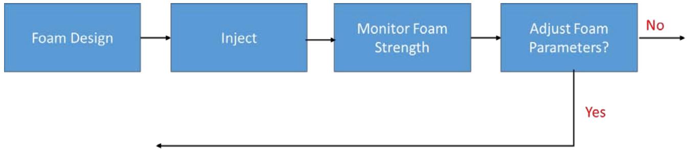 Fig. 2: Foam (and $\mathrm{CO}_{2}$ -Foam) optimization process (Karakas and Aminzadeh, 2017). In terms of laboratory studies, Berge (2017) conducted resistivity measurements while injecting $\mathrm{CO}_{2}$ and surfactant solution into saturated cores and Haroun et al. (2017) monitored resistivity and pressure changes during foam generation in the formation-brine saturated carbonate core plug samples. Haroun et al. (2017) reported significant increases in resistivity and pressure with foam development. The main thrust of this paper is to the characterize the resistivity response and to present a theoretical foundation for resistivity monitoring during $\mathrm{CO}_{2}$ foam displacements. ## II. $\mathrm{CO}_{2}$ FOAM TRANSPORT MODELING The transport of $\mathrm{CO}_{2}$ foam can be described by several methods (Ma, K. et al., 2015). These include: - Pore-network models - Analytical methods - Explicit population-based equation (PBE) methods - Implicit foam methods Pore-Network models provide a good insight into foam transport and are not yet practical for reservoir-scale applications. In this study, we focus on the Analytical and the explicit (or Population Based) methods. The analytical approach is based on the fractional-flow theory and steady-state foam development, as presented by Ashoori et al. (2010). The main assumptions are as follows: - One-dimensional flow. - Initially, the reservoir is at residual oil saturation $(S_{\mathrm{or}})$ after waterflooding. - $\mathrm{CO}_{2}$ is injected at supercritical conditions. - First-Contact Miscible (FCM) displacement of oil by the injected supercritical $\mathrm{CO}_{2}$. - The relative permeability depends on water saturation and the oil or $\mathrm{CO}_{2}$ saturations. - Foam effects are captured implicitly using steady-state assumption. As demonstrated by Ashoori et al. (2010), there are two different solutions: the first one relates to an ideal $\mathrm{CO}_{2}$ -foam displacement where the miscible $(\mathrm{CO}_{2})$ and surfactant (foam) fronts travel at the same speed. In this case, three separate banks develop in the reservoir: Foam or surfactant $(\mathrm{CO}_{2}$ plus water) bank, oil (with mobile water) bank, and water (with residual oil) bank. The second solution assumes a non-ideal $\mathrm{CO}_{2}$ -foam displacement. In this case, due to adsorption of the injected surfactant to the rock and its partitioning to the water phase, the foam front slows down, and the miscible $(\mathrm{CO}_{2})$ front moves ahead of it. In this case, a separate $\mathrm{CO}_{2}$ bank forms ahead of the foam (or surfactant) bank, which gives rise to an unfavorable mobility distribution in the reservoir. These reconstructed saturation profiles are provided in Appendix A. The fractional flow approach is based on the steady-state assumption and cannot capture the transient foam development during $\mathrm{CO}_{2}$ foam injection (Kam S.I., 2008). ## III. POPULATION-BALANCE METHOD In the Population Based (PBE) method, foam effects are captured explicitly by quantifying the bubble population $(n_{t})$ and correlating it to the foam mobility. In this work, we utilized the solution approach provided by Kam and Rossen (2003). The relevant foam equations are provided in Appendix B. Please note that this solution is based on the two-phase $\mathrm{(CO_2}$ and water) flow, and the oil phase is ignored. This assumption is in line with most experimental work and gives good insight into foam development in porous media (Kam et al., 2004, Prigiobbe et al., 2016). The solution of the PBE, due to nonlinear relations between injection rate and pressure gradient, is quite complex and may not be unique (Dholhawala, Z.F. et al., 2007). In this work, a numerical approach was taken for solving the transient foam equations. With this objective, a numerical foam simulator (FoamSim) was developed, in which upstream weighting was utilized to minimize the numerical dispersion effects. The numerical model was validated by comparing its results with that of Kam et al. (2004). These comparisons were made for both weak and strong foam states. ## IV. PARAMETER ESTIMATION USING PRESSURE MEASUREMENTS One of the crucial considerations is the uniqueness of the model parameters obtained from pressure measurements. For this reason, we analyzed the inter dependency between various foam parameters. These included foam generation parameters ( $\mathsf{C}_{\mathsf{g}}$ & m), foam coalescence parameters ( $\mathsf{C}_{\mathsf{c}}$ & n), and the foam viscosity parameter ( $\mathsf{C}_{\mathsf{t}}$ ). For this purpose, we utilized the published $\mathsf{CO}_{2}$ foam experiments by Prigiobbe et al. (2016). The foam parameters for these history matched experiments are as follows: Table 1: Model Parameters used for Foam Simulations (From Prigiobbe et al., 2016). <table><tr><td></td><td>Cf</td><td>Cg</td><td>Cc</td><td>M</td><td>n</td><td>Sw*</td></tr><tr><td>Experiment 6</td><td>1.58E-15</td><td>3.02E+07</td><td>3.02E-01</td><td>0.588</td><td>0.73</td><td>0.121</td></tr><tr><td>Experiment 34</td><td>3.31E-17</td><td>3.72E+06</td><td>9.55E-03</td><td>1.140</td><td>0.29</td><td>0.01</td></tr></table> We first ran forward simulations using FoamSim and compared our results with those of Prigiobbe et al. Two experiments (6 & 34) produced very similar (but not exact) results. The graph below shows the comparison for Experiment 6 using parameters from the table above. 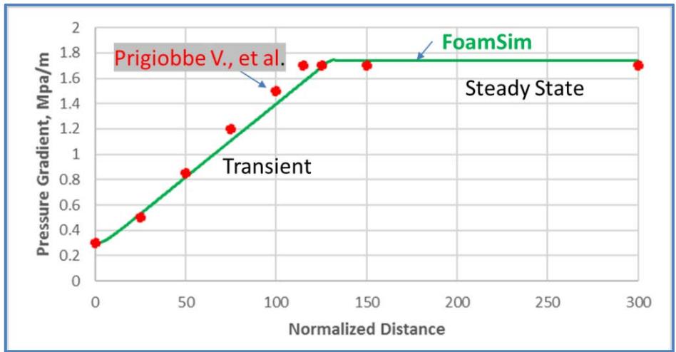 Fig. 3: Comparison of pressure gradients (experiment number 6). The relevant sensitivity coefficients were generated using our numerical solver (FoamSim), and for experiments 6 and 34 and the duration of the lab experiments. In this analysis, the following parameters were considered: $$ \mathrm{X} = \text{foamparameters} \left[ \mathrm{C} _ {\mathrm{g}}, \mathrm{C} _ {\mathrm{c}}, \mathrm{C} _ {\mathrm{f}}, \mathrm{m}, \mathrm{n} \right] \tag{1} $$ For most high-permeability systems, the critical water saturation $(S_{\mathrm{w}}^{*})$ is relatively small. Therefore, due to potential numerical problems, it was not included in the analysis. In the calculations of sensitivity coefficients, we used the log transformation for all the foam parameters: $$ C_{g}^{ extprime} = \log_{10}(C_{g}) $$ The following plot shows the calculated sensitivity coefficients using data from experiment number 6: 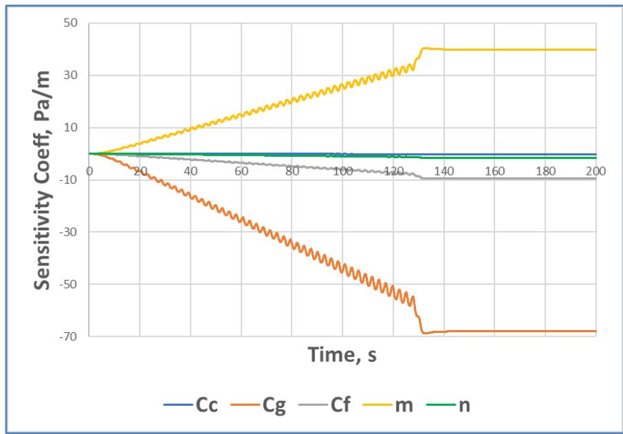 Fig. 4: Sensitivity coefficients for foam parameters (experiment number 6). We also normalized sensitivity coefficients for an even comparison and calculated the determinant of the sensitivity matrix to examine the (ill) conditioning of the inverse problem. The determinant (d) is a function of time and is defined as follows: $$ \mathrm {d} = \left[ \mathbf {S} ^ {\mathrm {T}} \mathbf {S} \right] \tag {3} $$ These calculations showed that the magnitude of the determinant increased with time (with more measurement samples): 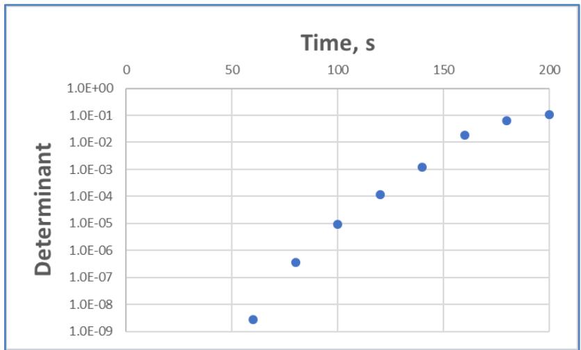 Fig. 5: Determinant of the sensitivity matrix. We also calculated the determinant using the steady-state portion of the measurements only. For steady-state flow, the determinant became very small, which indicates a linear dependency between the selected foam parameters (Appendix B). This examination showed the following: - Foam generation parameters, $C_g$ & m, have by far the highest sensitivity. - Foam viscosity coefficient, $C_{\mathrm{f}}$, is of the middle rank. - Foam coalescence parameters, $C_c$ & n, have relatively less sensitivity. - Linear independence is possible with transient data. - Steady-State pressure measurements give rise to an ill-conditioned parameter estimation problem and the grouping of parameters is necessary. ## V. $\mathrm{CO}_{2}$ FOAM RESISTIVITY CHARACTERISTICS AND MODELING Typically, nonionic surfactants are dissolved in the $\mathrm{CO}_{2}$ phase, and the foam generation occurs in situ when injected the $\mathrm{CO}_{2}$ plus surfactant meets the formation brine. $\mathrm{CO}_{2}$ is highly resistive, whereas the thin water film is conductive (depending on the salinity of the in-situ reservoir fluid). During foam injection, these films enhance the electrical conductivity. With growing bubble size, these conduits become less effective, and overall, the resistivity of the foam system increases. However, with $\mathrm{CO}_{2}$ injected brine already resistive this will only produce more resistive fluid. Reduction in resistivity will come from higher electron flow and resistivity reduction caused by pressure changes. See Boerner et al (2015) on electrical conductivity of $\mathrm{CO}_{2}$ -bearing pore waters at elevated pressure and temperature. Assuming a uniform and hexagonal-prism shape foam, the foam conductivity $\sigma_{f}$ is obtained using the Lemlich Relation (Lemlich, R., 1985): $$ \mathbf{K} = \frac{\mathrm{D}}{3} $$ Where $K$ is the bulk foam conductivity. This relationship can also be written as follows: $$ \mathrm{K} = \frac{\text{conductivityofdispersion}}{\text{conductivityofcontinousphase}} = \frac{\sigma_ {f}}{\sigma_ {s}} \tag{5} $$ Where D is the volumetric liquid fraction or $= (1-$ X), and X is the foam quality. Using these relationships, we obtain: $$ \sigma_{f} = \frac{1}{3} \sigma_{s} \left(1 - X_{\mathrm{f}}\right) \tag{6} $$ or another expression would be: $$ \sigma_ {f} = c _ {1} * \sigma_ {s} * \left(1 - S _ {c o 2} ^ {f}\right) \tag {7} $$ where: $$ c _ {1} = \text{constant} $$ $$ S _ {c o 2} ^ {f} = \mathrm{C O} _ {2} \text{saturationwithfoam} $$ $$ \sigma_ {s} = \text{conductivityofthethinfilmaroundbubbles} $$ Assuming, $\sigma_{s} = 1.0\mathrm{S / m}$ and $X_{\mathrm{f}} = 0.90$ (foam quality), we obtain the following values for foam conductivity: $\sigma_{f} = 0.033 \mathrm{~S} / \mathrm{m}$ (foam conductivity) or $R_{\mathrm{f}} = 30 \mathrm{ohm}.\mathrm{m}$ (foam resistivity) These results suggest that foam conductivity will be order of (1 to 2) higher compared to that of the $\mathrm{CO}_{2}$ phase only. We propose to scale the foam conductivity with foam density as follows: $$ \sigma_ {f} = c 1 \sigma_ {s} \left(1 - S _ {c o 2} ^ {f}\right) \left(\frac {n _ {f}}{n _ {f m a x}}\right) \tag {8} $$ where $n_{\text{film}}$ is the maximum population density. For a $\mathrm{CO}_{2}$ -Water system, lab results show that Archie's equation provides a reasonable approximation (Bergmannet al., 2013). Assuming a $\mathrm{CO}_{2}$ -Foam-Water system, the total system conductivity was calculated by utilizing the mixing law (Appendix D): $$ \sigma = \phi^{2} \left[ S_{co2}^{f} \sigma_{f}^{1/2} + S_{w} \sigma_{w}^{1/2} \right]^{2} $$ Laboratory measurements using carbonate cores from Abu Dhabi (Harounet al., 2017) show a sharp increase in resistivity and a large pressure drop with the formation of foam during these high-temperature and high-pressure core floods. These experimental results are in line with the theoretical results provided here. The difference between foam and $\mathrm{CO}_{2}$ saturated reservoir depends on how much $\mathrm{CO}_{2}$ is absorbed by the brine. However, strictly speaking, volumetrics are empirical correlations and do not often work for resistivity due to non-linearity of Archie. With fracture we increase complexity even further. ### a) Resistivity Profiles Using the simulated saturation and the foam densities, we can now estimate the resistivity (along with relative mobility) evolution during the $\mathrm{CO}_{2}$ -Foam displacements. For these simulations, we assumed the following bulk conductivities for water, $\mathrm{CO}_{2}$, foam, and oil phases: Table 2: Parameters Used For Resistivity Simulations <table><tr><td>σw</td><td>5.00</td><td>S/m</td></tr><tr><td>σco2</td><td>0.001</td><td>S/m</td></tr><tr><td>σf</td><td>0.100</td><td>S/m</td></tr><tr><td>σoil</td><td>0.001</td><td>S/m</td></tr></table> The figure below shows the resistivity profile from one dimensional $\mathrm{CO}_{2}$ foam flood assuming a moderately conductive water scenario. The resistivity profile has been calculated using the simulated foam densities from the FoamSim simulator, and the $\mathrm{CO}_{2}$ foam resistivity model. To avoid using canonical resistivity values one would in practice scale the surface measurements to the borehole scale as shown by Strack et al (2022). 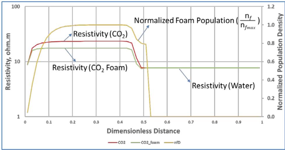 Fig. 6: Calculated resistivity profile during $\mathrm{CO}_{2}$ -Foam injection (PBE Solution). 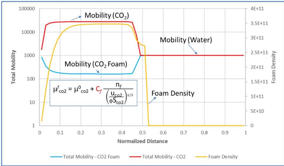 Fig. 7: Combined resistivity and mobility profile during $\mathrm{CO}_{2}$ -Foam injection (PBE Solution). ### b) Resistivity Profiles - ${\mathrm{{CO}}}_{2}$ Foam Displacement with Oil The resistivity calculations for the $\mathrm{CO}_{2}$ foam with oil were also made for $\mathrm{CO}_{2}$ -foam displacement with oil. For this model, the mobility effects were calculated using the steady-state assumption as outlined in Appendix A. The resistivity calculations were made assuming similar bulk conductivities as given in Table 2. The figures below show the calculated resistivity profiles for both ideal as well as non-ideal foam displacements: 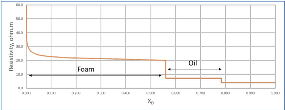 Fig. 8: Resistivity profile during ideal $\mathrm{CO}_{2}$ -Foam displacement. 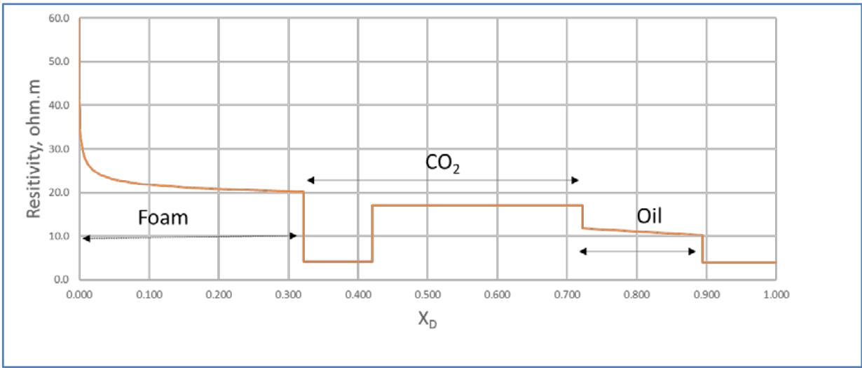 Fig. 9: Resistivity profile during non-deal $\mathrm{CO}_{2}$ -Foam displacement. The figures below show the mobility distribution along with the resistivity profiles. 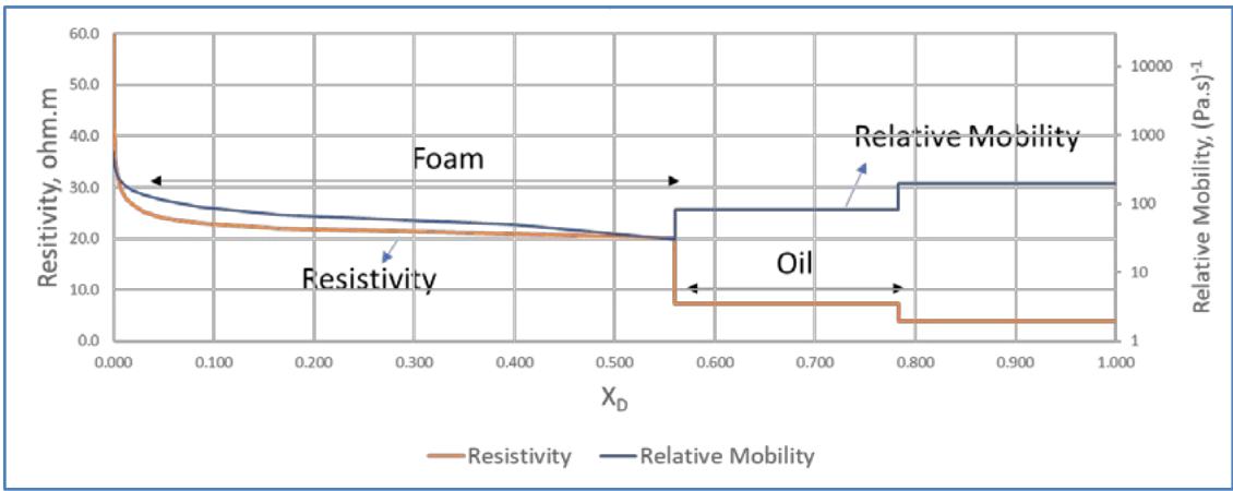 Fig. 10: Combined resistivity and mobility profile during $\mathrm{CO}_{2}$ -Foam injection (analytical Solution - ideal displacement). As seen in Fig. 10, the resistivity profile during ideal displacement is like the PBE simulations shown earlier, and both models suggest a sharp resistivity contrast at the foam front. On the other hand, for non- ideal displacements, the resistivity profile is quite different. During these displacements, the resistivity profile, as shown in Fig. 11, indicate a staircase behavior, which extends into the miscible $\mathrm{CO}_{2}$ bank. 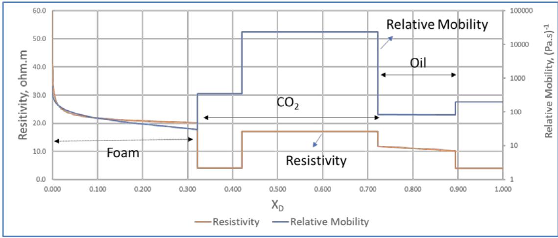 Fig. 11: Combined resistivity and mobility profile during $\mathrm{CO}_{2}$ -Foam injection (analytical solution - non-ideal displacement). ## VI. CONCLUSIONS In this paper, we presented a volumetric based foundation for resistivity and pressure monitoring during $\mathrm{CO}_{2}$ -foam displacements. Our results suggest that a combination of pressure and resistivity measurements in time-lapse mode could be deployed as an effective monitoring tool in field applications of the $(\mathrm{CO}_{2})$ foam processes. The proposed method is novel as it could be employed to predict under-performing $\mathrm{CO}_{2}$ -foam floods and to improve oil recovery and $\mathrm{CO}_{2}$ storage. Other conclusions can be listed as follows: - Pressure measurements during steady-state foam flow give rise to an ill-posed estimation problem and that grouping of foam parameters is necessary. For most reservoir applications, pressure measurements alone will not adequately describe the transient foam effects. - Assuming brine in the reservoir, resistivity profiles during ideal $\mathrm{CO}_{2}$ foam displacements should exhibit a distinctive signature at the foam front. - During non-ideal $\mathrm{CO}_{2}$ foam displacements, resistivity measurements by itself may not be enough to differentiate foam and miscible $\mathrm{CO}_{2}$ banks. However, for these non-ideal cases, pressure measurements could be very utilized to locate these vastly contrasting mobility-fronts. ### ACKNOWLEDGEMENTS We would like to acknowledge financial support from Chevron for this research. We also acknowledge the input from Kurt Strack of KMS Technology. $c_{1} = a$ constant in the proposed foam conductivity model $C_{c} =$ a model parameter to represent foam coalescence $C_f =$ a model parameter to represent effective foam viscosity $C_g = a$ model parameter to represent foam generation $\mathrm{D} =$ volumetric liquid fraction in the foam, fraction $d =$ value of determinant to capture the conditioning of the parameter estimation problem epdry = a foam parameter used to capture the slope near critical water saturation fmmob = a factor in steady-state foam model to represent the mobility factor fmdry = a factor in steady-state foam model to represent the critical water saturation epsurf = a steady-state foam parameter $f_{co2} = \mathrm{CO}_2$ phase fractional flow, fraction $f_{\mathrm{w}} =$ water phase fractional flow, fraction $\mathrm{Fw} =$ factor to capture the effect of water saturation on foam mobility reduction $K =$ bulk foam conductivity, $(S / m)$ $k =$ permeability, $\mathfrak{m}^2$ $\mathrm{k}_{\mathrm{rCO2}} =$ relative permeability to CO2 phase, fraction $k_{ro} =$ relative permeability to oil phase, fraction ${\mathrm{k}}_{\mathrm{{rw}}} =$ relative permeability to water phase, fraction $m = a$ model parameter for transient foam generation M = measurement matrix n = a model parameter for transient foam coalescence $R_{CO2} =$ resistivity of the $\mathrm{CO}_{2}$ phase, ohm-m $R_{f} =$ resistivity of the foam, ohm-m $R_{w} =$ resistivity of water phase, ohm-m $n_f =$ foam texture or density, lamellae/unit volume $n_{fmax} =$ maximum foam density, lamellae/unit volume $r_c =$ foam (lamella) destruction rate $r_g =$ foam (lamella) generation rate S = sensitivity matrix $\mathsf{S}_{\mathsf{co2}} = \mathsf{CO}_2$ saturation, fraction $\mathbf{S}_{\mathrm{o}} =$ oil saturation, fraction $S_{\mathrm{w}} =$ water saturation, fraction $\mathrm{u}_{\mathrm{co2}} = \mathrm{CO}_2$ volumetric flux or superficial velocity, m/s $u_{t} =$ total velocity, $m / s$ $u_{w} =$ water velocity, $m/s$ $\mathrm{vf} =$ volumetric fraction of rock and fluids, fraction $V_{s} =$ velocity of the foam front, m/s $v_{w} =$ velocity of the miscible $(\mathrm{CO}_{2})$ front, m/s $X =$ vector defining the foam parameters $X_{\mathrm{f}} =$ foam quality, fraction $\mu_{\mathrm{co2}}^0 = \mathrm{CO}_2$ viscosity (without foam), Pa.s $\mu_{\mathrm{co2}}^{\mathrm{f}} =$ effective viscosity of the $\mathrm{CO}_{2}$ foam phase, Pa.s $\phi =$ porosity, fraction $\sigma_{co2} = \mathrm{CO}_2$ conductivity (without foam), S/m $\sigma_{co2}^{\dagger} = \mathrm{CO}_{2}$ conductivity (with foam), S/m $\sigma_{f} =$ foam conductivity, S/m $\sigma_{w} =$ water conductivity, S/m $\nabla p =$ total pressure gradient, Pa/m $\nabla p_w =$ pressure gradient for the water phase, $\mathrm{Pa / m}$ #### Appendix A - Analytical Solution In the example provided by Ashoori et al. (2010), the following fluid and rock parameters are assumed: Table A1: Model Parameters used for Analytical Simulations <table><tr><td>μw</td><td>0.001</td><td>Pa.s</td></tr><tr><td>μo</td><td>0.005</td><td>Pa.s</td></tr><tr><td>μg</td><td>2E-05</td><td>Pa.s</td></tr><tr><td>φ</td><td>0.25</td><td></td></tr><tr><td>Sgr</td><td>0.1</td><td></td></tr><tr><td>Swc</td><td>0.1</td><td></td></tr><tr><td>Sor</td><td>0.1</td><td></td></tr></table> Water and Oil phase relative permeabilities are modeled as follows: $$ k _ {r w} = 0.2 0 * \left(\left(S _ {w} - 0.1\right) / 0.8\right) ^ {4.2} (\text{Water}) \tag{A1} $$ $$ k_{ro}=0.94*\left(\left(1-S_{w}-0.1\right)/0.8\right)^{1.3} \text{(Oil)} \tag{A2} $$ Water and $\mathrm{CO}_{2}$ phase relative permeabilities are represented by the following relationships: $$ k _ {r w} = 0.2 0 * \left(\left(S _ {w} - 0.1\right) / 0.8\right) ^ {4.2} (\text{Water}) \tag{A3} $$ $$ \mathrm{k} _ {\mathrm{r g}} ^ {0} = 0.9 4 * \left(\left(1 - S _ {\mathrm{w}} - 0.1\right) / 0.8\right) ^ {1.3} \quad \left(\mathrm{C O} _ {2} \text{withoutfoam}\right) \tag{A4} $$ In these models, foam reduces the $\mathrm{CO}_{2}$ relative permeability, using the steady-state assumptions, as follows: $$ \mathrm {k} _ {\mathrm {r g}} ^ {\mathrm {f}} = \mathrm {k} _ {\mathrm {r C g}} ^ {0} * \frac {1}{1 + f m m o b * \mathrm {F w a t e r}} \tag {A5} $$ Where: $$ F _ {\text{water}} = 0.5 + \pi^ {- 1} \tan^ {- 1} [ \text{epdry} (S w - f m d r y) ] \tag{A6} $$ where fmdry and epdry are empirical parameters based on experimental data. In the example by Ashoori et al., 2010, the following parameters were utilized: Table A2: Foam Parameters used for Analytical Simulations <table><tr><td>fmmob</td><td>55000</td></tr><tr><td>fmdry</td><td>0.316</td></tr><tr><td>epdry</td><td>1000</td></tr><tr><td>epsurf</td><td>100</td></tr></table> Using these parameters, fractional flow curves for foam/water, $\mathrm{CO}_{2}$ /water and oil/water phases were reconstructed. Also, we used the two separate solutions; the first solution assumes an ideal displacement where the miscible fronts and the surfactant (foam) fronts travel at the same speed. For this to happen, there must be a minimal Surfactant adsorption as well as very favorable partitioning of the surfactant into the $\mathrm{CO}_{2}$ phase. In the ideal displacement case, the solution paths are constructed by first drawing a tangent from the $M = D = (1,1)$ point to the curve representing the fractional flow of foam, as shown in the figure below: 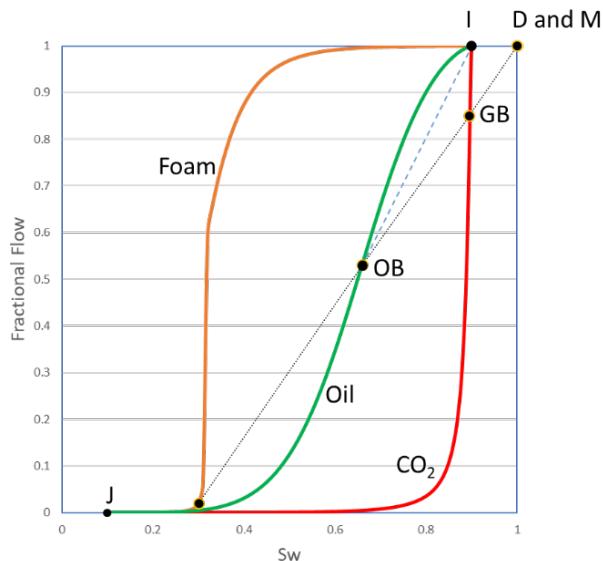 Fig. A1: Fractional flow - Ideal Displacement. The saturation profile for the ideal displacement case is as follows:  Fig. A2: Saturation profile - Ideal Displacement. The second solution is non-ideal displacement where the miscible fronts and the surfactant (foam) fronts travel at different speeds. In this case, the surfactant adsorption as well as partitioning of the surfactant into the water phase slows down the speed of the foam (surfactant) front. On the other hand, the miscible $(\mathrm{CO}_{2})$ front moves at the same speed as before. Therefore, miscible front shoots ahead of the foam (surfactant) front. Thus, a $\mathrm{CO}_{2}$ bank forms. In this case, there are four different banks, and the construction of the solution paths starts first by drawing tangents from point D and the miscibility point, point M (1,1) to curves representing the fractional flow of oil and foam, respectively. 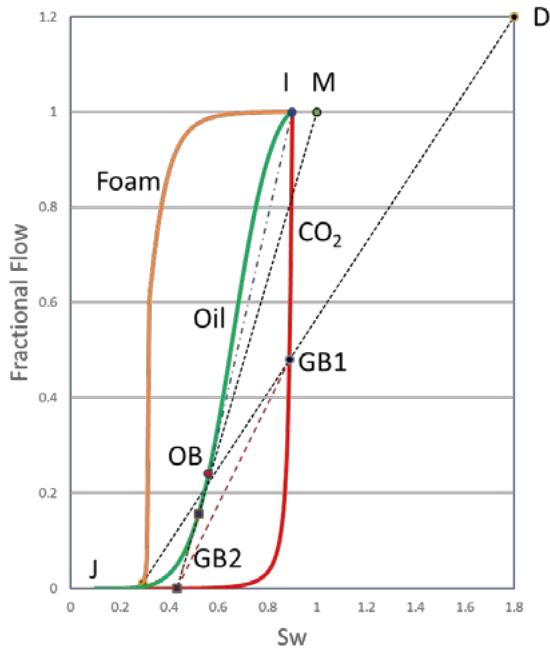 Fig. A3: Fractional flow, Non-Ideal displacement. The saturation profile for the non-ideal displacement case is as follows: 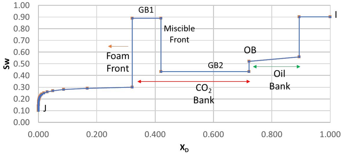 Fig. A4: Saturation profile, Non-Ideal displacement. #### Appendix B - Population based Foam Model Assuming one-dimensional flow of water and $\mathrm{CO}_{2}$, the material balance of water is described by the following equation: $$ \phi \frac {\partial S _ {w}}{\partial t} + u _ {t} \frac {\partial f _ {w}}{\partial x} = 0 \tag {B1} $$ In this model, total flow rate $(u_{t})$ is assumed to be constant. As usual, water fractional flow is written as follows: $$ f_{w} = \frac{\frac{k_{rw}}{\mu_{w}}}{\frac{k_{rw}}{\mu_{w}} + \frac{k_{rco2}}{\mu_{co2}^{f}}} \tag{B2} $$ $$ \mu_{co2}^{f} = \mu_{co2}^{0} + C_{f} \frac{n_{f}}{\left(\frac{u_{co2}}{\phi S_{co2}}\right)^{1/3}} \tag{B3} $$ In this equation, $C_f$ is an empirical parameter based on experimental data. Foam density $(n_f)$ equation is described by the following equation (Kovscek et al. 1995): $$ \phi \frac{\partial (S_{co2} n_f)}{\partial t} + u_t \frac{\partial (f_{co2} n_f)}{\partial x} = \varphi S_{co2} (r_g - r_c) \tag{B4} $$ The rate of foam generation is given by $$ r _ {g} = C _ {g} \nabla p ^ {m} \tag {B5} $$ and the rate of foam coalescence is given by $$ r _ {c} = C _ {c} n _ {f} \left(\frac {S _ {w}}{S _ {w} - S _ {w} ^ {*}}\right) ^ {n} \tag {B6} $$ Where $C_g, C_c, m$ and $n$ are model parameters. $S_w^*$ is the water saturation linked with the critical capillary pressure for a foam-water system. In high permeability reservoirs, $S_w^*$ is expected to be small. Also, the foam behavior around the critical water saturation could be quite abrupt. The water rate is given by $$ u _ {w} = - \frac {k k _ {r w}}{\mu_ {w}} \nabla p _ {w} \tag {B7} $$ and the foam rate is given by: $$ u _ {c o 2} = - \frac {k k _ {r c o 2}}{\mu_ {c o 2} ^ {o}} (\nabla p _ {w} - \nabla p _ {c}) \tag {B8} $$ At steady state conditions, the foam generation rate is equal to the foam destruction (or coalescence) rate. $$ r _ {g} = r _ {c} \tag {B9} $$ when this relationship is inserted into the foam-viscosity equation: $$ \mu_{co2}^{f} = \mu_{co2}^{0} + C_{f} \frac{n_{f}}{\left(\frac{u_{co2}}{\phi S_{co2}}\right)^{\frac{1}{3}}} \tag{B10} $$ the following relationship is obtained, representing the foam viscosity: $$ \mu_ {c o 2} ^ {f} = \mu_ {c o 2} ^ {0} + \frac {C _ {g} C _ {f}}{C _ {c}} \frac {\nabla p ^ {m}}{(\frac {S _ {w}}{S _ {w} - S _ {w} ^ {*}}) ^ {n} (\frac {u _ {c o 2}}{\phi S _ {c o 2}}) ^ {\frac {1}{3}}} \quad (\mathrm {B 1 1}) $$ #### Appendix C - Sensitivity Coefficients For a single-measurement (pressure) case, the Model response is defined as follows: $$ \mathbf{M} (\mathbf{X}) = \nabla p _ {\text{mod}} (\bar{\mathbf{X}}) \tag{C1} $$ Where $M$ is a matrix representing the model response and $X$ is a vector representing the system unknowns: $$ \mathrm{X} = \text{foamparameters} [ \mathrm{X} _ {1}, \mathrm{X} _ {2}, \mathrm{X} _ {3}, \dots \mathrm{X} _ {\mathrm{i}} \dots \dots , \mathrm{X} _ {\mathrm{p}} ] \tag{C2} $$ where $p$ is the total number of unknowns. In this case, the Sensitivity Coefficients are defined as follows: $$ \mathbf {S} (\mathbf {X}) = \left[ \nabla_ {\mathrm {x}} \mathbf {M} ^ {\mathrm {T}} (\mathbf {X}) \right] \tag {C3} $$ and the Sensitivity Matrix for the Single Response Case is defined as follows: $$ S = \left[ \begin{array}{c} M _ {1 1} \dots \dots \dots .. M _ {1 p} \\M _ {k 1} \dots \dots \dots .. M _ {k p} \end{array} \right] \tag {C4} $$ or $$ \mathsf{S} = \left[ \begin{array}{l l} \frac{\delta M_{1}}{\delta x_{1}} \dots \dots \dots . & \frac{\delta M_{1}}{\delta x_{p}} \\\frac{\delta M_{k}}{\delta x_{1}} \dots \dots \dots . & \frac{\delta M_{k}}{\delta x_{p}} \end{array} \right] \tag{C5} $$ where $k$ is the number of measurements. Sensitivity of the Model response $(M_{i})$ to parameter vector $X_{j}$ is defined as follows: $$ \mathrm {S} _ {\mathrm {i j}} ^ {(1)} = \frac {\delta M _ {i}}{\delta x _ {j}} | \mathrm {x} ^ {(1)} \tag {C6} $$ where $X^{(l)}$ represents the parameter vector which was used in generating the forward simulations. #### Appendix D - Conductivity of Fluid Mixtures Conductivity of fluid mixtures in porous media can be represented using the mixing law (Montaron, B., 2009). For a rock saturated with fluids, the total conductivity is expressed by the following equation: $$ \sigma^ {1 / 2} = \mathrm {v f} _ {1} \sigma_ {1} ^ {1 / 2} + \mathrm {v f} _ {2} \sigma_ {2} ^ {1 / 2} + \mathrm {v f} _ {3} \sigma_ {3} ^ {1 / 2} \tag {D1} $$ where $\sigma_{\mathrm{t}}$ and $\mathrm{v}f_{\mathrm{i}}$ represent the conductivity and the volumetric fraction of each component (rock and fluid), respectively. Additionally, the total volumetric fraction can be written as: $$ \mathrm{vf}_1 + \mathrm{vf}_2 + \mathrm{vf}_3 = 1.0 $$ for a water and oil/gas/CO $_2$ system these relationships become: $$ \sigma_ {1} = \sigma_ {R} = 0, \quad \mathrm {v f} _ {1} = 1 - \phi \tag {D3} $$ $$ \sigma_ {2} = \sigma_ {o} = 0, \quad \mathrm{v f} _ {2} = S _ {\mathrm{o}} \phi \tag{D4} $$ $$ \sigma_ {3} = \sigma_ {\mathrm{w}}, \quad \mathrm{v f} _ {3} = \sigma_ {\mathrm{w}} \phi \tag{D5} $$ and using the mixing law, we obtain: $$ \sigma = \sigma_ {\mathrm {w}} \left(\mathrm {S} _ {\mathrm {w}} \phi\right) ^ {2} \tag {D6} $$ This result is similar to Archie's law: $$ \sigma = \frac {\sigma_ {\mathrm {w}} S _ {\mathrm {w}} ^ {\mathrm {n}} \phi^ {\mathrm {m}}}{a} \tag {D7} $$ where $a$, $n$ and $m$ are constants. For a $\mathrm{CO}_{2}$ -Foam and water system, the mixing law equations become: $$ \sigma_ {1} = \sigma_ {R} = 0, \quad v f _ {1} = 1 - \phi \tag {D8} $$ $$ \sigma_ {2} = \sigma_ {f}, \quad \mathrm{v f} _ {2} = S _ {c o 2} ^ {f} \phi \tag{D9} $$ $$ \sigma_ {3} = \sigma_ {\mathrm{w}}, \quad \mathbf{v f} _ {3} = \sigma_ {\mathrm{w}} \phi \tag{D10} $$ and finally: $$ \sigma = \phi^ {2} \left[ S _ {c o 2} ^ {f} \sigma_ {f} ^ {1 / 2} + S _ {\mathrm{w}} \sigma_ {\mathrm{w}} ^ {1 / 2} \right] ^ {2} \tag{D11} $$

Generating HTML Viewer...

References

47 Cites in Article
Ajit Agnihotri,Robert Lemlich (1981). Electrical conductivity and the distribution of liquid in polyhedral foam.
E Ashoori,T Van Der Heijden,W Rossen (2010). Fractional-Flow Theory of Foam Displacements With Oil.
Reidar Nevdal,Halvor Gravdal,Jon Laberg,Kari Dyregrov (2017). Should the population limit its exposure to media coverage after a terrorist attack?.
P Bergmann,M Ivandic,B Norden,C Rücker,D Kiessling,S Lüth,C Schmidt-Hattenberger,C Juhlin (2013). Combination of seismic reflection and constrained resistivity inversion with an application to 4D imaging of the CO2 storage site, Ketzin, Germany.
J Bikerman (2013). Unknown Title.
J Boerner,H Volker,J Repke,Spitzer (2015). The electrical conductivity of CO2-bearing pore waters at elevated pressure and temperature: a laboratory study and its implications in CO2 storage monitoring and leakage detection.
Abderrezak Bouchedda*,Bernard Giroux (2015). Synthetic Study of CO<sub>2</sub> monitoring using Time-lapse Down-hole Magnetometric Resistivity at Field Reseach Station, Alberta, Canada.
Kin Chang,Robert Shiung,Lemlich (1980). A study of the electrical conductivity of foam.
N Christensen,D Sherlock,K Dodds (2006). Monitoring CO2 Injection with Cross-Hole Electrical Resistivity Tomography.
J Cilliers,M Wang,S Neethling (1999). Measuring flowing foam density distributions using ERT.
N Clark (1948). The electrical conductivity of foam.
J Cilliers,W Xie,S Neethling,E Randall,A Wilkinson (2001). Electrical resistance tomography using a bi-directional current pulse technique.
Z Dholkawala,H Sarma,S Kam (2007). Application of fractional flow theory to foams in porous media.
K Feitosa,S Marze,A Saint-Jalmes,D Durian (2005). Electrical conductivity of dispersions: from dry foams to dilute suspensions.
M Fernø,J Gauteplass,M Pancharoen,Å Haugen,A Graue,A Kovscek,G Hirasaki (2014). Experimental Study of Foam Generation, Sweep Efficiency and Flow in a Fracture Network.
N Gargar,H Mahani,J Rehling,S Vincent-Bonnieu,N Kechut,R Farajzadeh (2015). Fall-Off Test Analysis and Transient Pressure Behavior in Foam Flooding.
M Haroun,A Mohammed,B Somra,S Punjabi,A Temitope,Y Yim,S Anastasiou,J Baker,L Haoge,Al Kobaisi,F Aminzadeh,M Karakas,M Corova,F (2017). Real-Time Resistivity Monitoring Tool for In-Situ Foam Front Tracking.
G Hirasaki,J Lawson (1985). Mechanisms of Foam Flow in Porous Media: Apparent Viscosity in Smooth Capillaries.
Seung Kam (2008). Improved mechanistic foam simulation with foam catastrophe theory.
Seung Kam,Quoc Nguyen,Qichong Li,William Rossen (2007). Dynamic Simulations With an Improved Model for Foam Generation.
M Karakas,F Aminzadeh (2017). Optimization of CO2-Foam Injection through Resistivity and Pressure Measurements.
Dana Kiessling,Cornelia Schmidt-Hattenberger,Hartmut Schuett,Frank Schilling,Kay Krueger,Birgit Schoebel,Erik Danckwardt,Juliane Kummerow (2010). Geoelectrical methods for monitoring geological CO2 storage: First results from cross-hole and surface–downhole measurements from the CO2SINK test site at Ketzin (Germany).
J Kim,Y Dong,W Rossen (2005). Steady-State Flow Behavior of CO2 Foam.
J Kim,M Nam,T Matsuoka (2016). Monitoring CO2 drainage and imbibition in a heterogeneous sandstone using both seismic velocity and electrical resistivity measurements.
Jongwook Kim,Ziqiu Xue,Toshifumi Matsuoka (2010). Experimental Study on CO2 Monitoring and Saturation with Combined P-wave Velocity and Resistivity.
A Kovscek,C Radke (1994). Fundamentals of foam transport in porous media.
A Kovscek,T Patzek,C Radke (1995). A mechanistic population balance model for transient and steady-state foam flow in Boise sandstone.
V Kuuskraa,G Koperna (2006). The Status and Potential of Enhanced Oil Recovery.
R Lemlich (1985). Semitheoretical equation to relate conductivity to volumetric foam density.
Mohammad Lotfollahi,Rouhi Farajzadeh,Mojdeh Delshad,Abdoljalil Varavei,William Rossen (2016). Comparison of Implicit-Texture and Population-Balance Foam Models.
Kun Ma,Guangwei Ren,Khalid Mateen,Danielle Morel,Philippe Cordelier (2015). Modeling Techniques for Foam Flow in Porous Media.
H Mahani,T Sorop,P Van Den Hoek,A Brooks,M Zwaan (2011). Injection Fall-Off Analysis of Polymer Flooding EOR.
B Montaron (2009). How Well Does Archie Speak French?.
Yoshihiro Nakatsuka,Ziqiu Xue,Henry Garcia,Toshifumi Matsuoka (2010). Experimental study on CO2 monitoring and quantification of stored CO2 in saline formations using resistivity measurements.
M Namdar Zanganeh,W Rossen (2013). Optimization of Foam Enhanced Oil Recovery: Balancing Sweep and Injectivity.
Quoc Nguyen,George Hirasaki,Keith Johnston (2015). Novel CO<sub>2</sub> Foam Concepts and Injection Schemes for Improving CO<sub>2</sub> Sweep Efficiency in Sandstone and Carbonate Hydrocarbon Formations.
S Omar,M Jaafar,A Ismail,W Sulaiman (2013). Monitoring Foam Stability in Foam Assisted Water Alternate Gas (FAWAG) Processes Using Electrokinetic Signals.
Kyosuke Onishi,Yoshihiko Ishikawa,Yasuhiro Yamada,Toshifumi Matsuoka (2006). Measuring electric resistivity of rock specimens injected with gas, liquid and supercritical CO <sub>2</sub>.
Herminio Passalacqua,Sonya Davydycheva,Kurt Strack (2018). Feasibility of Multi-Physics Reservoir Monitoring for Heavy Oil.
Valentina Prigiobbe,Andrew Worthen,Keith Johnston,Chun Huh,Steven Bryant (2016). Transport of Nanoparticle-Stabilized CO $$_2$$ 2 -Foam in Porous Media.
C Schmidt-Hattenberger,P Bergmann,T Labitzke,F Wagner (2014). CO2 Migration Monitoring by Means of Electrical Resistivity Tomography (ERT) – Review on Five Years of Operation of a Permanent ERT System at the Ketzin Pilot Site.
K Strack,H Hinojosa,E Luschen,Y Martinez (2022). Using Electromagnetics for Geothermal and Carbon Capture, Utilization and Storage (CCUS) applications.
K.-M Strack (2014). Future Directions of Electromagnetic Methods for Hydrocarbon Applications.
H Tapp,A Peyton,E Kemsley,R Wilson (2003). Chemical engineering applications of electrical process tomography.
M Wang,J Cilliers (1999). Detecting non-uniform foam density using electrical resistance tomography.
Yuxin Wu,Susan Hubbard,Dawn Wellman (2012). Geophysical Monitoring of Foam Used to Deliver Remediation Treatments within the Vadose Zone.
Z Xue,J Kim,S Mito,K Kitamura,T Matsuoka (2009). Detecting and Monitoring CO2 With P-Wave Velocity and Resistivity From Both Laboratory and Field Scales.
No ethics committee approval was required for this article type.
Data Availability
Not applicable for this article.
How to Cite This Article
Metin Karakas. 2026. \u201cCO2-Foam Monitoring using Resistivity and Pressure Measurements\u201d. Global Journal of Research in Engineering - J: General Engineering GJRE-J Volume 22 (GJRE Volume 22 Issue J2).
Explore published articles in an immersive Augmented Reality environment. Our platform converts research papers into interactive 3D books, allowing readers to view and interact with content using AR and VR compatible devices.
Your published article is automatically converted into a realistic 3D book. Flip through pages and read research papers in a more engaging and interactive format.
Our website is actively being updated, and changes may occur frequently. Please clear your browser cache if needed. For feedback or error reporting, please email [email protected]
Thank you for connecting with us. We will respond to you shortly.