## I. INTRODUCTION Investing in a hydropower plant is very expensive, but it has an operating life of more than 30 years, with very low operating and maintenance costs compared to other power plants. In addition, in recent years, the experience gained in forecasting risks and production have facilitated the financing of hydropower projects, including private investments. The field of hydropower also boasts state-of-the-art technology. These days, turbines have attained efficiencies of over $97\%$ and are extremely reliable. These data hence ensure that we have installations that function properly and also reduces the risk of downtime. The function of penstocks is to transfer water from the reservoirs to the installations (turbines in a hydroelectric plant) that convert hydraulic energy into electrical energy [1]. They are made up of sections with singularities where the local hydrodynamic pressures take on high values, as they follow the shape of the relief: slopes, obstacles, crossing of troughs, etc. The hydraulic plant therefore supports a pressure that is of the order of the head, but the effects of head loss reduce this value [1]. For a conduit flow, forces normal to walls are not involved; only tangential and therefore viscous forces contribute to the drag and power input [2]. The pressure drop thus depends on the type of flow, determined by the Reynolds number, and on the internal roughness of the pipe. It should be noted that the absolute roughness represents the average thickness of the surface roughness of the pipe material [3]. The gradient of the linear head loss, also called friction slope, depends on the friction coefficient, the flow volume and the geometrical characteristics of the structure [4], [5]. The friction coefficient is a function of the Reynolds number characterizing the flow, and the relative roughness of the pipe under consideration [6]. Since the roughness in a penstock is closely related to the coefficient of friction, an accurate estimate of roughness is crucial to plant performance. According to ENEO [7], the Songloulou hydroelectric plant is the largest (384 MW) and the Lagdo plant one of the most recent (72 MW) of the Cameroonian plants. The first is the largest dam on the South Interconnected Network (RIS), and the second the only hydroelectric power station on the North Interconnected Network (RIN). The objective of this work is to approach the reality of the field with regard to the environment of these dams, based on their structures. We will therefore characterize the friction in the penstock of each. This study is one of the preliminary analyses of the flow in the penstock of a Cameroonian hydroelectric dam. No previous study on the friction parameters in the penstocks of the two dams studied is available. Therefore, this study will examine the hydraulic characteristics influenced by the penstock walls on the flow within the penstock and at its outlet. The study focuses on the evolution of the friction coefficient in the whole structure, obtained analytically by the conventional method and by a graphical approach. Our analysis will enable us to identify the most interesting method for approximating the exact value of the coefficient of friction. It may also give rise to a new approach to monitoring these delicate structures. ## II. 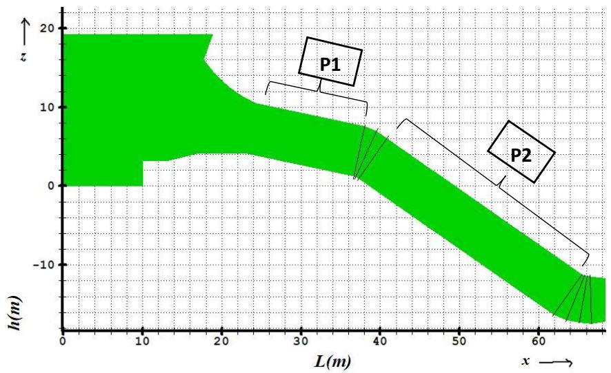MATERIALS The materials on which our study is based are the Songloulou and Lagdo dams. Figures 1 and 2 below show the mesh of the structures in question (the Songloulou and the Lagdo dams study area respectively).  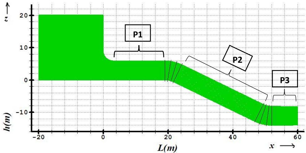 Figure 1: Songloulou Dam mesh We modeled our power plants in Gambit 2.2. For Figure 1, the mesh type used is regular with 675845 quadrilateral meshes, 1108245 faces and 661186 nodes. For figure 2, the type of mesh used is regular with 197455 quadrilateral faces. On these figures, we have highlighted the portions in which we will present the results obtained (i.e. portions 1, 2 and 3 in the case of Lagdo). Thus for the case of Songloulou, we have P1 for the first portion of the pipe and P2 for the second portion. The same is true for the case of Lagdo where we have three portions, including P1, P2 and P3. Note that these portions represent the straight portions from which the results will be presented. ## III. METHODS ### a) Theoretical Approach To determine the friction coefficient $f$ of a turbulent flow, the empirical equation developed by Colebrook-White remains the reference equation. This equation is well known among hydraulic engineers, and continues to be the subject of research. The calculations and plots in this work are obtained from the following equation (equation 1) [8]. $$ \frac {1}{\sqrt {f}} = - 2 l o g _ {1 0} \left[ \frac {\varepsilon / D}{3 . 7} + \frac {2 . 5 1}{R e \sqrt {f}} \right] \tag {1} $$ Where $\varepsilon D$ is the relative roughness (derived from the absolute roughness $\varepsilon$ and the diameter $D$ ), Re the Reynolds number and $f$ the desired coefficient of friction. For the pressure drop, equation 2 below is used from the friction coefficient obtained previously [4], [5]. $$ J = \frac {8 f}{g \pi^ {2}} \frac {Q ^ {2}}{D ^ {5}} \tag {2} $$ In the case of the conduit, another definition of the drag coefficient $\lambda$ is used, called the friction coefficient \[2\]: $$ \lambda = \frac {d}{1 / 2 \rho U _ {o} ^ {2}} \frac {\Delta P}{l} \tag {3} $$ ### b) Numerical Approach The Fluent software is used for this approach, as it has a large number of turbulence models to cope with many physical problems. The geometry of the structure as well as the type of boundary conditions of the physical domain of the parameters that characterize the fluid-structure interaction were modelled in Gambit version 2.2. Knowing that the fluid is incompressible, the motion is described using differential equations with derivatives in the following form \[9\]: $$ \frac {\partial u}{\partial x} + \frac {\partial v}{\partial y} + \frac {\partial w}{\partial z} = 0 \tag {4} $$ For the u component parallel to the wall, the stationary Navier-Stokes equation simplifies considerably in the very near wall. $$ u \frac {\partial u}{\partial x} + v \frac {\partial u}{\partial y} = - \frac {1}{\rho} \frac {\partial p}{\partial x} + v \frac {\partial^ {2} u}{\partial x ^ {2}} + v \frac {\partial^ {2} u}{\partial y ^ {2}} \tag {5} $$ The convective terms tend to zero (adhesion condition) and the term $\frac{\partial^2 u}{\partial x^2}$ is negligible in front of the term $\frac{\partial^2 u}{\partial y^2}$ (weakly non-parallel flow condition). In short, all that remains is: $$ \frac{1}{\rho} \frac{\partial p}{\partial x} = v \frac{\partial^2 u}{\partial y^2} $$ It can be seen that the pressure gradient in the boundary layer imposes the curvature $\frac{\partial^2 u}{\partial y^2}$ of the velocity profile $u(y)$. The energy equation is represented by the relation below \[10\]: $$ \frac{\partial T}{\partial t} + u \frac{\partial T}{\partial x} + v \frac{\partial T}{\partial y} + w \frac{\partial T}{\partial z} = a \left(\frac{\partial^2 T}{\partial x^2} + \frac{\partial^2 T}{\partial y^2} + \frac{\partial^2 T}{\partial z^2}\right) \tag{7} $$ The decomposition of the viscous stress tensor is written: $$ \underline {{\underline {{\tau}}}} = \underline {{\underline {{\tau}}}} + \underline {{\underline {{\tau}}}} ^ {\prime} \tag {8} $$ with the viscous stress tensor given by: $$ \left\{ \begin{array}{l} \overline{\tau_{ij}} = \mu \left(\frac{\partial \overline{u_{i}}}{\partial x_{j}} + \frac{\partial \overline{u_{j}}}{\partial x_{i}}\right) - \frac{2}{3} \mu \frac{\partial \overline{u_{k}}}{\partial x_{k}} \delta_{ij} \\ \tau_{ij}^\prime = \mu \left(\frac{\partial u_{i}^\prime}{\partial x_{j}} + \frac{\partial u_{j}^\prime}{\partial x_{i}}\right) - \frac{2}{3} \mu \frac{\partial u_{k}^\prime}{\partial x_{k}} \delta_{ij} \end{array} \right. \tag{9} $$ The equations of the turbulent kinetic energy and its dissipation rate give us: $$ \left\{ \begin{array}{c} \rho \bar {u} _ {j} \frac {\partial \varepsilon}{\partial x _ {j}} = \frac {\mu_ {i}}{\sigma_ {k}} \frac {\partial^ {2} k}{\partial x ^ {2} j} + \rho p _ {k} - \rho \varepsilon \\ \rho \bar {u} _ {j} \frac {\partial \varepsilon}{\partial x _ {j}} = \frac {\mu_ {i}}{\sigma_ {\varepsilon}} \frac {\partial^ {2} \varepsilon}{\partial x ^ {2} j} + \rho \frac {\varepsilon}{k} \left(c _ {\varepsilon 1} p _ {k}\right) - c _ {\varepsilon 2} \varepsilon \end{array} \right. \tag {10} $$ The turbulence model is $k\varepsilon$ and the resolution method is RANS. The flow and site (location) parameters of each structure were considered in obtaining the different results. The Colebrook-White formula was integrated into the fluent solver via a calculation code. ## IV. RESULTS AND DISCUSSION ### a) Theoretical Approach The theoretical approach is based on the Colebrook-white's formula [8] for a steel pipe in an evolving state, i.e. from new $(\varepsilon = 0.03\mathrm{mm})$ to worn $(\varepsilon = 1\mathrm{mm})$. We note that these values are those defined by hydraulic engineers and available in literature to characterize the evolution of roughness in steel pipes, as is the case in our dams. ## i. Case of the Songloulou Dam Starting from five velocities corresponding to the variation of velocity in the water intake for the periods of low water and flood, we calculated the friction coefficient $f$ for four values of the absolute roughness $\varepsilon$. Table 1 below shows the results obtained. Table 1: Evolution of the friction coefficient in our pipe as a function of \\varepsilon <table><tr><th>Velocity (V)</th><th>Ab. Roughness (\varepsilon)</th><th>Relative roughness (\varepsilon/D)</th><th>Friction Coef. (f)</th></tr><tr><td rowspan="4">4,045; 4,1.</td><td>0.05</td><td>0,00781</td><td>0,03495</td></tr><tr><td>0.09</td><td>0,01406</td><td>0,04270</td></tr><tr><td>0.3</td><td>0,04688</td><td>0,06946</td></tr><tr><td>0.8</td><td>0,12500</td><td>0,11550</td></tr><tr><td rowspan="4">4,3; 4,5; 4,73.</td><td>0.05</td><td>0,00781</td><td>0,03495</td></tr><tr><td>0.09</td><td>0,01406</td><td>0,04270</td></tr><tr><td>0.3</td><td>0,04688</td><td>0,06946</td></tr><tr><td>0.8</td><td>0,12500</td><td>0,11549</td></tr></table> We find that the friction coefficient remains almost identical in the pipe with increasing Reynolds number for a given $\varepsilon$. Similarly, the only element influencing the friction coefficient $f$ in this formula is $\varepsilon$. In the same logic, we have looked for the influence of these parameters on another structure, in order to compare the results obtained. ## ii. Case of the Lagdo Dam The approach is identical to that used for the Songloulou dam, with the speed ranges corresponding to the variation of speed in the water intake for the periods of low water and flood for this structure. Table 2 below presents the results obtained. Table 2: Evolution of the friction coefficient in our pipe according to $\varepsilon$ <table><tr><td>Velocity (V)</td><td>Ab. Roughness (ε)</td><td>Relative roughness (ε/D)</td><td>Friction Coef. (f)</td></tr><tr><td rowspan="4">3,1; 3,3</td><td>0.05</td><td>0,00833</td><td>0,03571</td></tr><tr><td>0.09</td><td>0,01500</td><td>0,04371</td></tr><tr><td>0.3</td><td>0,05000</td><td>0,07156</td></tr><tr><td>0.8</td><td>0,13333</td><td>0,12003</td></tr><tr><td rowspan="4">3,5; 3,7; 3,87</td><td>0.05</td><td>0,00833</td><td>0.03570</td></tr><tr><td>0.09</td><td>0,01500</td><td>0,04371</td></tr><tr><td>0.3</td><td>0,05000</td><td>0,07156</td></tr><tr><td>0.8</td><td>0,13333</td><td>0,12003</td></tr></table> The observation is the same as that made from Table 1. The friction coefficient remains practically the same in the pipe with the increase of the Reynolds number for a given $\varepsilon$. We can therefore conclude that for these results that whatever the other parameters in the Colebrook-White's formula, only the absolute roughness has an impact on the result obtained. However, in view of the two tables above, the coefficient of friction is also influenced by the flow rate (with higher values in the Lagdo dam penstock, which has a lower flow rate). We also note that the head loss corresponding to this approach according to formula 2 can only be static in a considered portion. ### b) Numerical Approach This is the friction coefficient obtained graphically on each point constituting the portions of the penstock. The idea is to identify the evolution of the turbulent friction in each portion of the penstock according to the parameters of its environment. To do this, we seek by the same approach the maximum thickness of the asperities influencing the structure of the flow (what we will call real absolute roughness). Note that the fluid considered here is clear water with a density of $1000\mathrm{kg} / \mathrm{m}^3$. ## i. Case of the Songloulou Dam a. Research of the real value of $\varepsilon$ In order to find out the real thickness of the roughness influencing the friction coefficient in the pipe, we proceeded by the creation of graphic study zones. These study areas leave the walls towards the axis of the penstock at a small pitch (1mm to 5mm). Figure 3 below illustrates the evolution of turbulent friction in the penstock for three defined absolute roughness steps (starting $\varepsilon = 15\mathrm{mm}$ towards the wall), with an initial velocity of $4.045 \mathrm{~m} / \mathrm{s}$. Note that the same test was carried out on the upper wall. 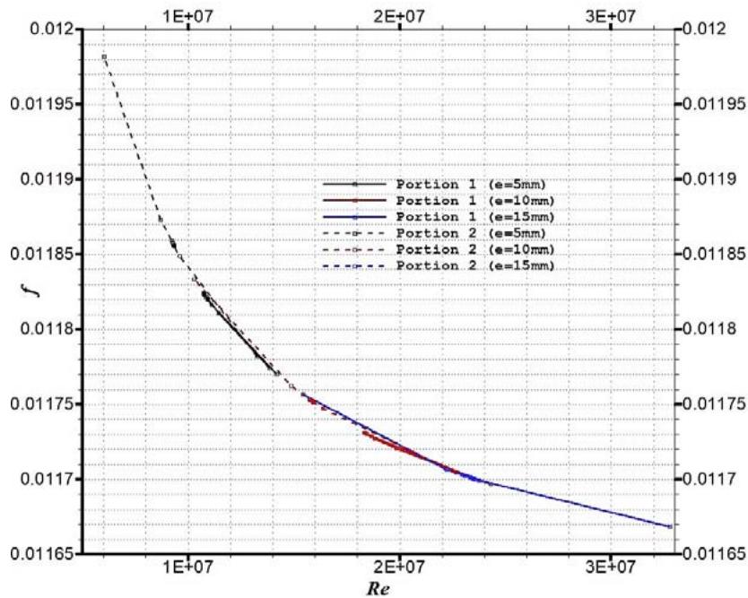 Figure 3: Evolution of turbulent friction in the pipe for $e = \varepsilon_{\mathrm{max}}$ different The idea here is to see at what thickness e we have maximum friction. This thickness will then be considered as our maximum relative roughness $(\varepsilon_{\text{max}})$. We can see from this figure that the maximum value of $f$ is observed for $e = 5\text{mm}$ $(\varepsilon_{\text{max}} = 5\text{mm})$. This is justified by the fact that as we approach the axis of our pipe ( $e > 5\text{mm}$ ), turbulent friction begins to drop considerably. It is in this logic that in the continuation of our work on this dam, we will carry out the evaluation of turbulent friction  a) on a thickness of 5mm. It should also be noted that these plots are made only in the different portions. b. 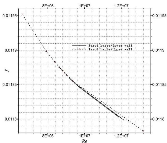Determination of the evolution of the friction coefficient $f$ in the penstock Figure 4 below shows the evolution of the friction coefficient $f$ as a function of the actual parameters of the structure. Thus, for a good appreciation of the values, the result will be presented for each section separately.  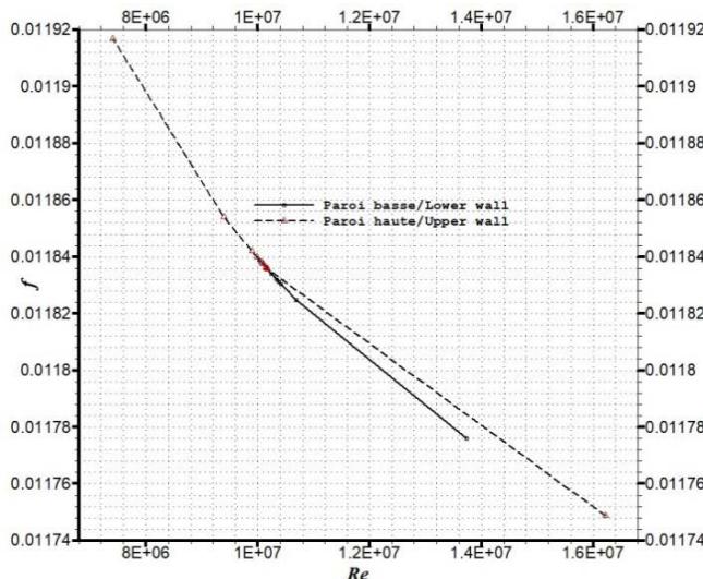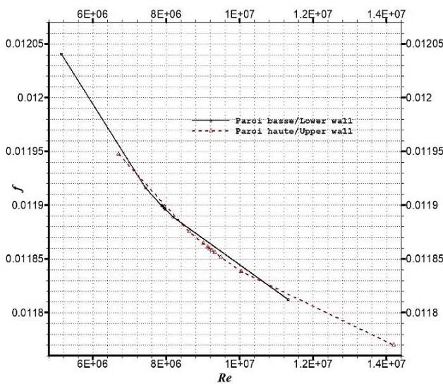b) Figure 4: Evolution of the friction coefficient in section 1 (a) and section 2 (b) for $\mathrm{Re} = 26.9 \times 10^{6}$ We can see that the turbulent friction varies from one wall to the other. Also, it is not identical in the two portions. It is dominant on the upper wall in the first portion of the penstock of our dam (Figure 4.a). On the other hand, in the second portion of our penstock (Figure 4.b), it is dominant on the lower wall with a higher value than the one observed in Figure 4.a. We will verify this hypothesis by applying this approach to another structure. ## ii. Case of the Lagdo Dam a. Finding the real value of $\varepsilon$ We proceed in the same way as in the case of the previous structure. Figure 5 below shows the turbulent friction in the pipe for $\varepsilon \leq 15\mathrm{mm}$ on the low wall, with an initial speed of $3.1\mathrm{m / s}$. 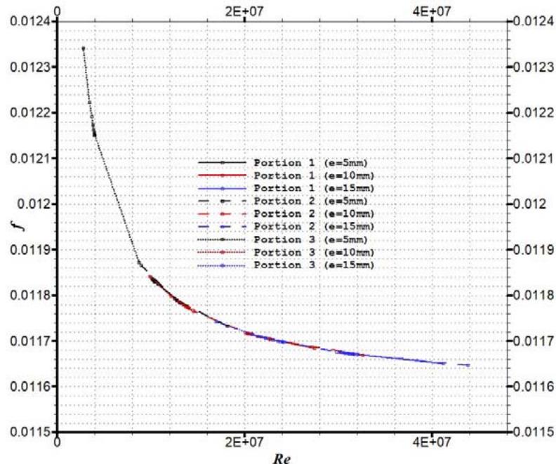 Figure 5: Evolution of the turbulent friction in the pipe for $e = \varepsilon_{\mathrm{max}}$ different As in the previous case, the maximum value of $f$ is still found when $\varepsilon = 5\mathrm{mm}$ as shown in Figure 5 above. This is the case for the lower and upper walls. b. Determination of the evolution of the friction coefficient $f$ in the penstock Figure 6 below shows the evolution of the friction coefficient $f$ as a function of the actual parameters of the structure. The result is presented separately for each of the three sections for a good appreciation of the values.  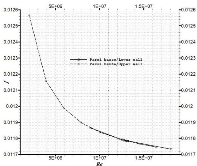a)  Figure 2: Lagdo Dam meshing   b)  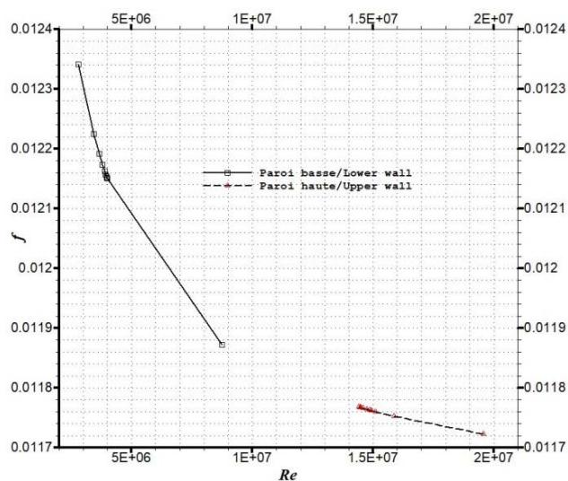c) Figure 6: Evolution of turbulent friction in section 1 (a), section 2 (b) and section 3 (c) for different Re We observe once again that the friction coefficient is not identical on the walls of the same section of pipe. It will be even less for each portion of our penstock. Apart from the third section of the pipe where turbulent friction is dominant on the lower wall (Figure 6.c), we rather have maximum turbulent friction on the upper wall for the other two sections (Figures 6.a and 6.b). As a general remark, we observe that the friction coefficient is neither identical on the same wall nor identical in the same portion, as presented by the theoretical approach. More importantly, it is not identical on the same section of the pipe. As another remark, the impact of the Reynolds number is visible on the evolution of the friction and was not felt on the results of the theoretical approach for our case. As a final remark, the head loss resulting from the numerical approach cannot be static in any portion of the pipe. This is not the case in the theoretical approach, given the shape of the curves obtained. Some researchers have already pointed out this shortcoming in the theoretical approach (for example Levin [11]). ### c) Validation of the Numerical Model To validate our model, the studies of Moss and Baker [12] and Abdalla et al. [13] were used. Figure 7 below shows the results obtained under similar study conditions. It shows the velocity profile over a reversal peak. 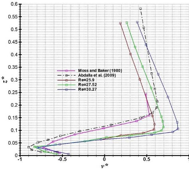 Figure 7: Flow structure on the sill for In this figure, our study is presented by the Reynold's numbers $Re$. In addition to the determination on the reversal peak, we have applied it to our case which is the Songloulou dam. The cause of the backdrop of our profiles is the transition from a free surface flow to a loaded flow, which doesn't exist in the study of Abdalla et al [13]. In the same logic, Abdalla et al [13] in their study evaluate the impact of the threshold (peak) on the energy dissipation at this level. They observe the pointed shape which explains the recirculation phenomenon. This is also evident in our case as shown in Figure 8 below. 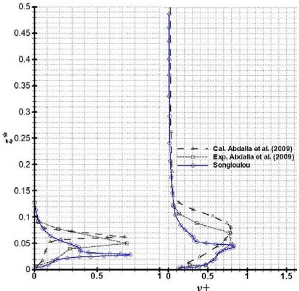 Figure 8: Turbulent intensity structure on the sill at $x = 11 \, \text{m}$ (left) and $x = 13 \, \text{m}$ (right) ## V. CONCLUSION The aim of this study was to investigate the impact of penstock walls on flow characteristics within the penstock and at its outlet. More precisely, it was to determine the evolution of the friction coefficient in the whole penstock. To carry out this work, two approaches were used. A theoretical approach, based on the direct determination by a commonly used formula (Colebrook-White's formula in this case), and another approach, the graphical, based on the numerical modelling of the structure under study. In the theoretical approach, five velocities corresponding to the variation of velocity in the water intake for periods of low and high water were used. The coefficient of friction $f$ was calculated for four values of absolute roughness $\varepsilon$. The results of this approach for our structures show that whatever the other parameters in the Colebrook-White formula (Reynolds number, diameter and absolute roughness), only absolute roughness has a visible impact on the result obtained. This can't be true, as clogging reduces the diameter and consequently modifies the flow rate. In the numerical approach, we looked for the maximum thickness of the asperities influencing the structure of the flow; what we called real absolute roughness. We have thus observed that the maximum value of $f$ is found for $e = 5\mathrm{mm}$ on the low and high walls. The results obtained from this approach show that the coefficient of friction is neither identical on the same wall, nor identical in the same portion. More importantly, it is not identical on the same section of the conduit, contrary to the theoretical approach which is a fixed result in a portion of pipe. In the same way, the impact of the Reynolds number is visible on the evolution of the friction coefficient in the numerical approach. This is not felt in the results of the theoretical approach for our cases. These remarks demonstrate the limitations of the theoretical approach to evaluating and determining head loss in hydraulic structures. The numerical approach would appear to be more useful for planning the maintenance of such structures, and also for optimizing their performance. We note, however, that apart from the geometric parameters of each structure studied, the usual data available in literature were used (absolute roughness, diameter and density of clear water). It is therefore recommended to take into account the characteristics of the sediments present in each site for the research to be upgraded.

Generating HTML Viewer...

References

9 Cites in Article
E Frédéric (2014). Rapport annuel sur les Principes directeurs de l'OCDE à l'intention des entreprises multinationales 2013.
C Olivier (2013). Introduction à la turbulence.
F Guidett,M Caleffi,M Doninelli,M Doninelli,C Ardizzoia,J Carlier,R Meskel (2005). Les pertes de charge dans les installations: Le dimensionnement des mitigeurs.
J Weisbach (1845). Unknown Title.
H Darcy (1857). Recherches Experimentales Relatives au Mouvement de L'Eau dans les Tuyaux, 2 volumes.
C Colebrook (1939). TURBULENT FLOW IN PIPES, WITH PARTICULAR REFERENCE TO THE TRANSITION REGION BETWEEN THE SMOOTH AND ROUGH PIPE LAWS..
S Eneo Energy of Cameroon.
C Colebrook,C White (1937). Experiments with fluid friction in roughened pipes.
T Tchawe,T Djiako,B Kenmeugne,D Tcheukam-Toko (2018). Numerical Study of the Flow Upstream of a Water Intake Hydroelectric Dam in Stationary Regime.
No ethics committee approval was required for this article type.
Data Availability
Not applicable for this article.
How to Cite This Article
Tchawe Tchawe Moukam. 2026. \u201cComparative Analysis of Friction Coefficient Evolution in Hydroelectric Dam Penstocks: Theoretical vs. Numerical Methods\u201d. Global Journal of Research in Engineering - A : Mechanical & Mechanics GJRE-A Volume 24 (GJRE Volume 24 Issue A2).
Explore published articles in an immersive Augmented Reality environment. Our platform converts research papers into interactive 3D books, allowing readers to view and interact with content using AR and VR compatible devices.
Your published article is automatically converted into a realistic 3D book. Flip through pages and read research papers in a more engaging and interactive format.
Our website is actively being updated, and changes may occur frequently. Please clear your browser cache if needed. For feedback or error reporting, please email [email protected]
Thank you for connecting with us. We will respond to you shortly.