I. INTRODUCTION

Image processing is the technique of performing operations on an image to enhance the quality of the image, extract useful information from it, or manipulate it for better usage. Digital image processing techniques are applied in fields of computer vision, pattern recognition, video processing, image restoration and image correction [1].

Image restoration [2] and correction entails all the techniques used to restore a damaged image. It includes noise removal from the image, correcting a blurred photo, enhancing an image with defocused subject, converting a black and white image to color image, removing stains and unwanted marks from the image, etc. Image inpainting is one such technique that falls under image restoration.

Image inpainting $[3]$ is a form of image restoration and conservation. The technique is generally used to repair photos with missing areas due to damage or aging, or mask out unpleasant deformed areas of the image. The use of inpainting can be traced back to the 1700s when Pietro Edwards, director of the Restoration of the Public Pictures in Venice, Italy, applied his scientific methodology to restore and preserve historic artworks. The modern approach to inpainting was established in 1930 during the International Conference for the Study of Scientific Methods for the Examination and Preservation of Works of Art. Technological advancements led to new applications of inpainting. Since the mid-1990's, the method of inpainting has evolved to include digital media. Widespread use of digital inpainting techniques range from entirely automatic computerized inpainting to tools used to simulate the process manually. Digital inpainting includes the use of software that relies on sophisticated algorithms to replace lost or corrupted parts of the image data. There are various advanced inpainting methodologies [4], namely Partial Differential Equation (PDE) based inpainting [5], Texture synthesis based inpainting [6], Hybrid inpainting [7], Example based inpainting [8] and Deep generative model based inpainting [9].

In this paper, we have presented a detailed comparative study of the three inpainting algorithms natively provided by the Open CV library, and also stated which is the most effective algorithm out of them. The paper is structured as follows: Section II contains the related work done in the past on comparative analysis of inpainting techniques and algorithms. Section III contains a brief theory behind the inpainting algorithms to be discussed. Section IV contains the details of the comparative study and experimental setup. Section V presents the results we obtained from our study and their critical explanations. Section VI details the possibilities of further work that can be performed on this topic. Section VII concludes the paper. We have focused more on the practical analysis of the three algorithms, and less on the theoretical and mathematical interpretation of the algorithms.

II. RELATED WORK

The first inpainting algorithm provided by OpenCV is established on the paper "An Image Inpainting Technique based on the Fast Marching method" by Alexandru Telea [10] in 2004. It is based on the Fast Marching Method. The second inpainting algorithm provided by OpenCV is established on the paper "Navier-Stokes, Fluid Dynamics, and Image and Video Inpainting" by M. Bertalmio et al [11] in 2001. It is based on fluid dynamics. The third inpainting algorithm was reviewed in the paper "Demonstration of Rapid Frequency Selective Reconstruction for Image Resolution Enhancement" by Nils Genser et al [12] in

2017. It is based on the Rapid Frequency Selective Reconstruction (FSR) method. They applied the algorithm on Kodak and Tecnick image datasets over custom error masks and presented the Peak Signal to Noise Ratio (PSNR), Structural Similarity Index (SSIM) and runtime metrics. We have used the same metrics for comparison, explained later in Section IV.

Supriya Chhabra et al [13] presented a critical analysis of different digital inpainting algorithms for still images, and also a comparison of the computational cost of the algorithms. We have considered execution time and memory consumption as metrics to compare computational cost between the algorithms. Raluca Vreja et al [14] published a detailed analytical overview of five advanced inpainting algorithms and measurement benchmarks. They emphasized on the advantages and disadvantages of the used algorithms and also proposed an improved adaptation of the Oliviera's [15] and Hadhoud's [16] inpainting algorithms.

Kunti Patel et al [17] presented a study and analysis of image inpainting algorithms and concluded that exemplar based techniques are generally more effective than PDE based or texture synthesis based techniques. They also extensively listed the merits and demerits of the algorithms, which makes it easy to choose for end users without further research. Anupama Sanjay Awati et al [18] detailed a review of digital image inpainting algorithms, comparing hybrid techniques against commonly used ones. K. Singh et al [19] presented a comparison of patch based inpainting techniques and proposed an adaptive neighborhood selection method for efficient patch inpainting.

III. THEORY

OpenCV is a library of programming functions mainly aimed at real-time computer vision. It is a huge open source library for computer vision, machine learning, image and video processing tasks. OpenCV is used in a lot of machine learning problems like face recognition, object detection, image segmentation, etc. mainly due to its simple syntax and presence of a large number of predefined functions and modules.

There are several algorithms present for digital image inpainting, but OpenCV natively provides three of them, INPAINT_TELEA, INPAINT_NS and INPAINT_FSR, which further has two profiles, FSR_FAST and FSR_BEST. INPAINT_TELEA and INPAINT_NS can be accessed by the function cv2.inpaint(). INPAINT_FSR can be accessed by the function cv2.xphoto.inpaint().

{"code_caption":[{"type":"text","content":"Fig. 1: Code to run the inpainting algorithms"}],"code_content":[{"type":"text","content":"In [1]: import cv2\n\nIn [2]: original = cv2.imread("original.jpg")\nmask = cv2.imread("mask.jpg", 0)\ninpaint_1 = cv2.inpaint(original, mask, 3, cv2.INPAINT_TELEA)\ninpaint_2 = cv2.inpaint(original, mask, 3, cv2.INPAINT_NS)\ncv2.xphoto.inpaint(original, mask, inpaint_3, cv2.xphoto.\nINPAINT_FSR_FAST)\ncv2.xphoto.inpaint(original, mask, inpaint_4, cv2.xphoto.\nINPAINT_FSR_BEST)"}],"code_language":"python"}

This section will contain a brief theory behind the three inpainting algorithms.

a) INPAINT_TELEA

This algorithm is based on the paper "An Image Inpainting Technique based on the Fast Marching method" by Alexandru Telea [10] in 2004. It is based on the Fast Marching Method (FMM), a solutional paradigm which builds a solution outwards starting from the "known information" of a problem. It is a numerical method created by James Sethian for solving boundary value problems of the Eikonal equation [20]. A simple explanation of the working of the algorithm follows, extracted from the original paper [10].

The first and foremost step in any inpainting method is to identify the region to be inpainted. There is the region to be inpainted, also known as the unknown region and the surrounding known region of the image.

The algorithm first considers the boundary of the unknown region, which is of infinitesimal width, and inpaints one pixel lying on the boundary. Then it iterates over all the pixels lying on the boundary to inpaint the whole boundary. A single pixel is inpainted as a function of all other pixels lying in its known neighborhood by summing the estimates of all pixels, normalized by a weighting function. A weighting function is necessary as it ensures the inpainted pixel is influenced more by the pixels lying close to it and less by the pixels lying far away. After the boundary has been inpainted, the algorithm propagates forward towards the center of the unknown region.

To implement the propagation, the Fast Marching Method (FMM) is used. FMM ensures the pixels near the known pixels are inpainted first, so that it mimics a manual inpainting technique. The FMM's main advantage is that it explicitly maintains a narrow band that separates the known from the unknown image area and specifies which pixel to inpaint next.

b) INPAINT_NS

This algorithm provided by OpenCV is established on the paper "Navier-Stokes, Fluid Dynamics, and Image and Video Inpainting" by M. Bertalmio et al [11] in 2001. This algorithm is based on fluid dynamics (fluid dynamics is a sub-discipline of fluid mechanics that describe the flow of fluids: liquids and gases) and utilizes partial differential equations. The method involves a direct solution of the Navier-Stokes equation [21] for an incompressible fluid. A simple explanation of the working of the algorithm follows, extracted from the original paper [11].

The basic principle is heuristic. After the user selects the unknown region, the algorithm first travels along the edges from known regions to unknown regions, and automatically transports information into the inpainting region. The algorithm makes use of isophotes (a line in a diagram connecting points where the intensity of light or brightness is the same). The fill-in is done is such a way that the isophote lines arriving at the unknown region's boundary are completed inside, which allows the smooth continuation of information towards the center of the unknown region. M. Bertalmio et al [11] drew an analogy between the image intensity function of an image and the stream function in a 2D incompressible fluid, and used techniques from the computational fluid dynamics to produce an approximate solution to image inpainting problem.

c) INPAINT FSR

FSR stands for Rapid Frequency Selective Reconstruction [12]. It is a high quality signal extrapolation algorithm. FSR has proven to be very efficient in the domain of inpainting. The FSR is a powerful approach to reconstruct and inpaint missing areas of an image.

The signal of a distorted block is extrapolated using known samples and already reconstructed pixels as support. This algorithm iteratively generates a generic complex valued model of the signal, which approximates the undistorted samples in the extrapolation area of a particular size as a weighted linear combination of Fourier basic function. The Fourier basic function is a method to smooth out data varying over a continuum (here the unknown region) and exhibiting a cyclical trend. An important feature of FSR algorithm is that the calculations are carried out in the Fourier domain, which leads to fast implementation.

There are two implementations of the FSR inpainting algorithm - INPAINT_FSR_FAST and INPAINT_FSR_BEST. The Fast implementation of FSR provides a great balance between speed and accuracy, and the Best implementation mainly focuses on the accuracy, with speed being slower compared to Fast.

IV. COMPARATIVE STUDY

a) Theoretical Comparison

All the three inpainting algorithms provided by OpenCV are unique and works on different methodologies. The similarity between the algorithms is the inpainting procedure starts with the pixels lying in the boundary of the unknown region, and slowly propagates towards the centre of the unknown region. All the three algorithms are heuristic in nature. The propagation method used in each is different. TELEA uses the Fast Marching Method (FMM), NS uses fluid dynamics equations and FSR extrapolates the pixel values of the unknown region using known samples.

b) Practical Comparison

For practical comparison of the 3 algorithms, we ran some code in Python. Our testing setup had the following specifications:

• CPU: i7-8700K (3.70 GHz)

• RAM: 16 GB (3200 MHz)

• GPU: 8 GB GTX 1080

We took the Kodak image set (which contains 25 uncompressed PNG true colour images of size 768x512 pixels) and four custom error masks for the dataset. We applied all the inpainting algorithms individually over each error mask on the images. We compared the results using four main metrics:

• Peak Signal to Noise Ratio (PSNR): It is the ratio between the maximum possible power of a signal and the power of corrupting noise. To estimate the PSNR of an image, it is necessary to compare the distorted image to an ideal clean image with the maximum possible power. PSNR is commonly used to estimate the efficiency of compressors, filters etc. A higher value of PSNR suggests an efficient manipulation method. In our case, we will compute the PSNR between the original image and the inpainted image. The Python code to calculate PSNR is given in Fig 2.

{"code_caption":[],"code_content":[{"type":"text","content":"In [1]: import cv2\n\nIn [2]: original = cv2.imread("original.jpg")\nmask = cv2.imread("mask.jpg", 0)\ninpainted = cv2.inpaint(original, mask, 3, cv2.INPAINT_TELEA)\npsnr = cv2.PSNR(original, inpainted, 255)"}],"code_language":"kotlin"}

Fig. 2: PSNR code

• Structural Similarity Index (SSIM): It is a perceptual metric that quantifies image quality degradation caused due to any kind of manipulation on the image. It is an improvement over the use of Mean Squared Error (MSE) to find similarity between images. In our case, we will compute the SSIM between the original image and the inpainted image. A higher value of SSIM suggests the inpainted image is structurally closer to the original

error mask 1 image. The Python code to calculate SSIM is given in Fig 3.

{"code_caption":[{"type":"text","content":"Fig. 3: SSIM code"}],"code_content":[{"type":"text","content":"In [1]: import cv2\nfrom skimage.metrics import structural_similarity as SSIM\n\nIn [2]: original = cv2.imread("original.jpg")\nmask = cv2.imread("mask.jpg", 0)\ninpainted = cv2.inpaint(original, mask, 3, cv2.INPAINT_TELEA)\nssim = SSIM(original, inpainted, multichannel=True)"}],"code_language":"python"}

• Runtime: It is the total time taken by the algorithm to complete its task. The Python code to calculate the runtime is given in Fig 4.

{"code_caption":[{"type":"text","content":"Fig. 4: Runtime code"}],"code_content":[{"type":"text","content":"In [1]: import cv2\nimport time\n\nIn [2]: original = cv2.imread("original.jpg")\nmask = cv2.imread("mask.jpg", 0)\nbegin = time.time()\ninpainted = cv2.inpaint(original, mask, 3, cv2.INPAINT_TELEA)\ntime.sleep(1)\nend = time.time()\nruntime = end-begin"}],"code_language":"lua"}

• Memory: It is the total memory consumed by the algorithm while completing the task. We use tracemalloc module, which is a debug tool to trace memory blocks allocated by Python. We find the peak memory usage during the working of the algorithm.

{"code_caption":[{"type":"text","content":"Fig. 5: Memory code"}],"code_content":[{"type":"text","content":"In [1]: import cv2\nimport tracemalloc\n\nIn [2]: original = cv2.imread("original.jpg")\nmask = cv2.imread("mask.jpg", 0)\ntracemalloc.start()\ninpainted = cv2.inpaint(original, mask, 3, cv2.INPAINT_TELEA)\ncurrent, peak = tracemalloc.get_traced_memory()\ntracemalloc.stop()\nmemory = peak/10**6"}],"code_language":"python"}

All the values have been taken up to three decimal places. Apart from the four main metrics, we also considered two hybrid metrics defined in Section V. We also curated some custom images for testing of certain specific cases. The results obtained are given in the next section, along with their critical explanation.

V. RESULTS AND DISCUSSION

a) Kodak image dataset results

There are 19 landscape and 6 portrait oriented photos in the Kodak image set. We initially made the custom error masks for landscape orientation, and rotated them to fit the portrait orientation. We chose striped masks as the error regions are equally distributed. The four custom error masks we considered are:

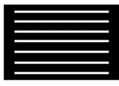
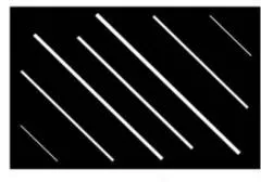
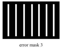
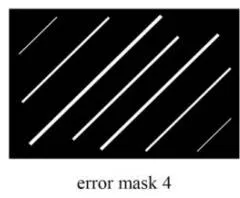
The white stripes are the areas to be inpainted. We have displayed the image results for just 1 landscape photo (2 error masks) and 1 portrait photo (2 error masks). These are the following results we obtained:-

Sample_1 (Landscape)

The original, distorted and 4 inpainted results of the first image sample over the first error mask are given in Fig 7.

original

TELEA

distorted NS

FSR_FAST

FSR_BEST Fig. 7: First image sample results over first error mask

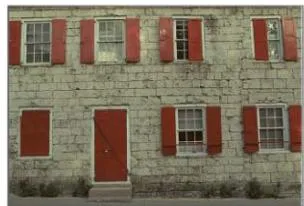
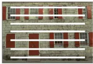
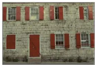
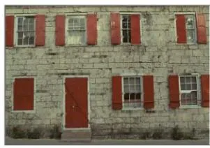
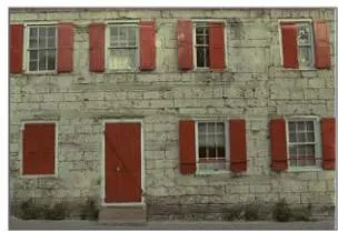
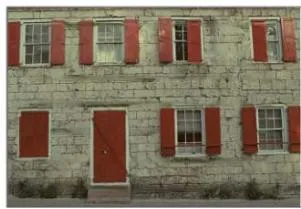
The metric values calculated for the first image sample over the first error mask are given in Table 1.

	FSR		TELEA	NS
	Fast	Best
PSNR [dB]	27.218	26.713	26.612	26.315
SSIM	0.889	0.889	0.887	0.884
Runtime [s]	5.349	96.199	1.089	1.085
Memory [MB]	1.339	1.339	1.339	1.339

The original, distorted and 4 in painted results of the first image sample over the second error mask are given in Fig 8.

original

distorted

TELEA

FSR_FAST

NS FSR_BEST Fig. 8: First image sample results over second error mask

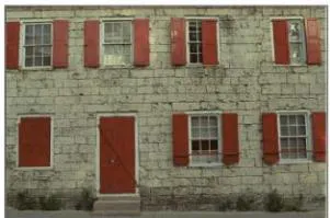
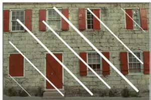
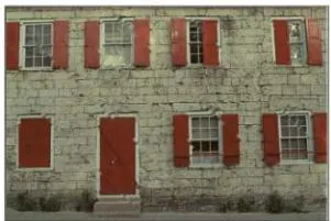
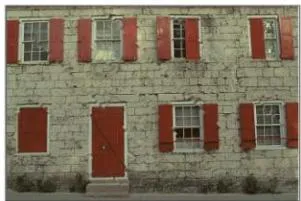
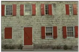
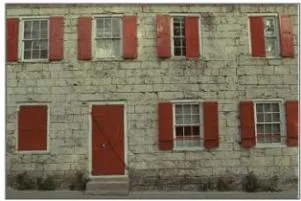
The metric values calculated for the first image sample over the second error mask are given in Table 2.

	FSR		TELEA	NS
	Fast	Best
PSNR [dB]	34.577	34.764	30.556	30.689
SSIM	0.974	0.975	0.950	0.952
Runtime [s]	2.887	35.132	1.049	1.047
Memory [MB]	1.339	1.339	1.339	1.339

	FSR		TELEA	NS
	Fast	Best
PSNR [dB]	27.143	27.229	27.096	26.796
SSIM	0.890	0.892	0.888	0.883
Runtime [s]	5.210	97.800	1.091	1.091
Memory [MB]	1.339	1.339	1.339	1.339

	FSR		TELEA	NS
	Fast	Best
PSNR [dB]	34.788	34.897	30.709	31.209
SSIM	0.975	0.976	0.952	0.955
Runtime [s]	3.114	39.762	1.055	1.049
Memory [MB]	1.339	1.339	1.339	1.339

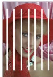
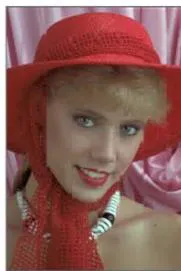
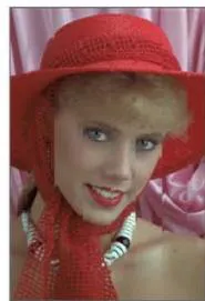
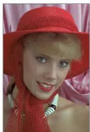
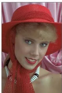
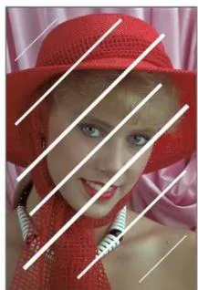
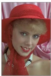
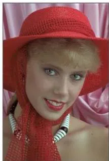
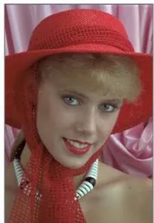
For portrait images, the error masks have been rotated 90 degree clockwise to fit the orientation. Given are the original, distorted and 4 in painted results of the second image sample over the first error mask in Fig 9.

original

distorted

TELEA

FSR_FAST

NS FSR BEST Fig. 9: Second image sample results over first error mask

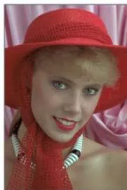
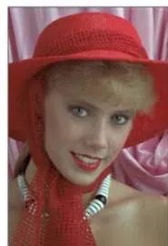
The metric values calculated for the second image sample over the first error mask are given in Table 5.

	FSR		TELEA	NS
	Fast	Best
PSNR [dB]	31.739	32.738	31.398	31.133
SSIM	0.936	0.941	0.934	0.932
Runtime [s]	4.574	65.644	1.092	1.088
Memory [MB]	1.339	1.339	1.339	1.339

original

distorted

TELEA

NS

FSR_FAST

FSR BEST Fig. 10: Second image sample results over second error mask

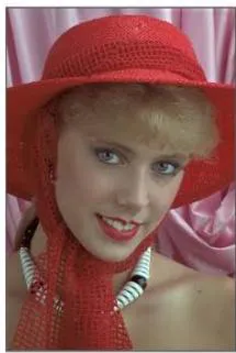
The metric values calculated for the second image sample over the first error mask are given in Table 6.

	FSR		TELEA	NS
	Fast	Best
PSNR [dB]	39.632	39.673	36.063	35.106
SSIM	0.983	0.983	0.972	0.971
Runtime [s]	2.568	23.655	1.044	1.052
Memory [MB]	1.339	1.339	1.339	1.339

	FSR		TELEA	NS
	Fast	Best
PSNR [dB]	32.105	31.834	30.596	30.268
SSIM	0.933	0.936	0.929	0.927
Runtime [s]	4.334	67.520	1.089	1.085
Memory [MB]	1.339	1.339	1.339	1.339

	FSR		TELEA	NS
	Fast	Best
PSNR [dB]	39.689	39.532	37.029	37.092
SSIM	0.985	0.985	0.975	0.975
Runtime [s]	2.634	25.407	1.056	1.057
Memory [MB]	1.339	1.339	1.339	1.339

	FSR		TELEA	NS
	Fast	Best
PSNR [dB]	29.719	30.017	29.145	28.891
SSIM	0.929	0.932	0.925	0.923
Runtime [s]	4.346	72.229	1.089	1.091
Memory [MB]	1.339	1.339	1.339	1.339

	FSR		TELEA	NS
	Fast	Best
PSNR [dB]	34.002	37.734	33.421	33.406
SSIM	0.952	0.983	0.968	0.969
Runtime [s]	3.546	27.488	1.047	1.048
Memory [MB]	1.339	1.339	1.339	1.339

	FSR		TELEA	NS
	Fast	Best
PSNR [dB]	28.948	29.143	28.602	28.376
SSIM	0.925	0.927	0.922	0.920
Runtime [s]	4.282	73.604	1.095	1.093
Memory [MB]	1.339	1.339	1.339	1.339

	FSR		TELEA	NS
	Fast	Best
PSNR [dB]	37.831	38.039	34.088	33.958
SSIM	0.983	0.984	0.970	0.969
Runtime [s]	2.725	31.751	1.052	1.051
Memory [MB]	1.339	1.339	1.339	1.339

consumption and runtime values mean a better algorithm. For other metrics, the higher the PSNR and SSIM value, the better the algorithm. The average memory consumption, as seen from Table 9,10,11,12 is same for any mask on any image for any algorithm for the particular dataset. Hence we will not consider it as a factor for deciding the most efficient algorithm. We have defined two hybrid metrics X and Y for deciding which algorithm is most efficient based on our data. Metric X is directly proportional to PSNR, directly proportional to SSIM and inversely proportional to Runtime value:

X α PSNR X α SSIM X α (1/Runtime)

Combining all three above equations we get:

where k is a constant, taken to be 1 for comparison purposes. Hence

A high value of metric X means an effective algorithm. We used the values obtained in Table 9,10,11,12 and calculated metric X values for the four error masks. The values are given in Table 13.

	FSR		TELEA	NS
	Fast	Best
$1^{st}$ Error Mask	6.353	0.387	24.756	24.442
$2^{nd}$ Error Mask	9.129	1.349	30.899	30.888
$3^{rd}$ Error Mask	6.253	0.367	24.083	23.885
$4^{th}$ Error Mask	13.647	1.179	31.431	31.309

From Table 13, we can see that TELEA algorithm gets the highest value in all four error masks. Hence, TELEA is the most efficient in painting algorithm when we consider metric X to be the comparison metric.

But as we can infer from the definition of metric X, it has the runtime factor associated with it. Runtime is an important factor for analysing algorithms, but can be subjective at times to different end users. Some users may have a time constraint, some users may not. Hence we need to define such a metric which does not include the runtime factor. Therefore, we define metric Y. Metric Y is directly proportional to PSNR and directly proportional to SSIM value:

Y α PSNR Y α SSIM

Combining all two above equations we get:

where k is a constant, taken to be 1 for comparison purposes. Hence

A high value of metric Y means an effective algorithm, without taking the runtime factor into account. Similarly, we used the values in Table 9,10,11,12 and calculated metric Y values for the four error masks. The values are given in Table 14.

	FSR		TELEA	NS
	Fast	Best
$1^{st}$ Error Mask	27.609	27.976	26.959	26.666
$2^{nd}$ Error Mask	32.369	37.093	32.352	32.370
$3^{rd}$ Error Mask	26.779	27.016	26.371	26.106
$4^{th}$ Error Mask	37.188	37.430	33.065	32.905

From Table 14, we can see that FSR_BEST algorithm gets the highest value in all four error masks. Hence, FSR_BEST is the most efficient inpainting algorithm when we consider metric Y to be the comparison metric, which does not take the runtime factor into account.

Summing up our observation and results for the Kodak image dataset, we can say that the most efficient inpainting algorithm when runtime is a constraint is TELEA algorithm and the most efficient inpainting algorithm when runtime is not a constraint is FSR_BEST algorithm.

b) Edge inpainting results

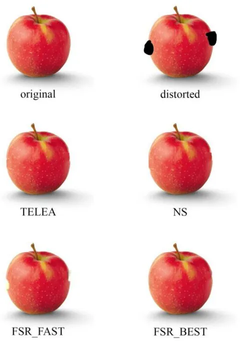
The inpainting algorithms produce very different results when working on edges. To compare the working, we have chosen an image which has clear distinct foreground and background. We distorted a part of the edge, and applied the inpainting algorithms to it. The image results are given in Fig 11, and metric values are given in Table 15.

As we can see from the results, TELEA has the highest value for X metric. That is if we consider runtime to be a factor, TELEA is the most efficient algorithm. But FSR_BEST has the highest value for Y metric, i.e. if we do not consider runtime to be a factor, then FSR_BEST is the most efficient algorithm for edge inpainting. We can also see from the image results that FSR_BEST produces the most believable result, but also has the largest runtime. TELEA and NS do a decent job in filling up the edges and maintaining the edge difference. But still some parts are hazed and distorted. FSR_FAST does the worst job, mainly because it trades off accuracy for runtime, and the result is bad.

	FSR		TELEA	NS
	Fast	Best
PSNR [dB]	35.249	43.100	38.577	37.973
SSIM	0.995	0.996	0.994	0.994
Runtime [s]	1.642	21.282	1.028	1.023
Memory [MB]	2.079	2.079	2.079	2.079
X	21.359	2.017	37.301	36.897
Y	35.073	42.928	38.346	37.745

c) Pattern inpainting results

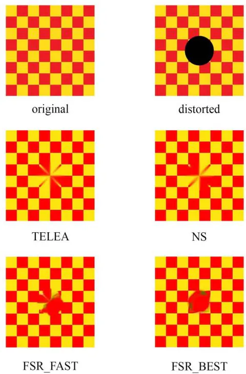
The inpainting algorithms produce very different results when working on patterns. To compare the working, we have chosen a checkerboard image as it is the easiest pattern to replicate. We distorted a part of the image in the centre, and applied the inpainting algorithms to it. The image results are given in Fig 12, and metric values are given in Table 16.

As we can see from the image results, none of the inpainting algorithms can replicate the pattern in the unknown region, which is understandable because the inpainting algorithms are focused on filling up the unknown region progressively based on information from the nearest known region. They work on the small scale spatial influences. In order to inpaint a pattern, the algorithm must work over a broad range of the known region to understand the dynamics of the pattern. An exemplar based inpainting or patch based inpainting method can work for pattern inpainting.

Comparing the metric values, TELEA has the highest X value and FSR_BEST has the highest Y value. From the image results, TELEA still does a decent job of producing an arbitrary pattern, while FSR_BEST fills the whole unknown region with a singular colour. Hence, no algorithm provided by OpenCV is perfectly suitable for inpainting a pattern, but TELEA can be used as a last resort.

	FSR		TELEA	NS
	Fast	Best
PSNR [dB]	20.094	21.881	19.017	18.872
SSIM	0.959	0.964	0.962	0.958
Runtime [s]	2.827	60.066	1.051	1.047
Memory [MB]	1.188	1.188	1.188	1.188
X	6.816	0.351	17.407	17.268
Y	19.270	21.093	18.294	18.079

d) Text error mask inpainting results

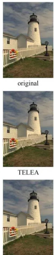
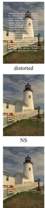
We also tested the working of the inpainting algorithms on a custom text error mask. We took an image from the Kodak dataset and wrote some random text on it as error regions, then applied the algorithms on it. The image results are given in Fig 13, and metric values are given in Table 17.

Comparing the metric values, NS has the highest X value and FSR_BEST has the highest Y value. All the algorithms work decent, but from the image results we can see that TELEA and NS have some distortions near the fence area, while FSR_FAST and FSR_BEST have inpainted smoothly in that area. If runtime is a constraint, then NS is the most effective algorithm to be used. Although, TELEA can also be used as it produces very similar results to NS. If runtime is not a constraint, then FSR_BEST is the most effective choice for text error mask inpainting.

	FSR		TELEA	NS
	Fast	Best
PSNR [dB]	45.019	45.497	30.784	31.571
SSIM	0.995	0.996	0.962	0.967
Runtime [s]	4.019	36.729	2.659	2.133
Memory [MB]	1.339	1.339	1.339	1.339
X	11.146	1.234	11.137	14.313
Y	44.794	45.315	29.614	30.529

FSR_FAST

FSR_BEST Fig. 13: Text error mask inpainting sample results

e) Monochromatic image inpainting results

We tested the working of the inpainting algorithms on a monochromatic image. We took an image from the Kodak dataset and converted it into monochrome and used a spiral error mask on it. The image results are given in Fig 14, and metric values are given in Table 18.

Comparing the metric values, NS has the highest X value and FSR_BEST has the highest Y value. All the algorithms work decent, but from the image results, we see that TELEA and NS have some distortions near the beak of the bird, while FSR_FAST and FSR_BEST have inpainted smoothly in that area. If runtime is a constraint, then NS is the most effective algorithm to be used. Although, TELEA can also be used as it produces very similar results to NS. If runtime is not a constraint, then FSR_BEST is the most effective choice for monochromatic image inpainting.

	FSR		TELEA	NS
	Fast	Best
PSNR [dB]	45.649	46.040	36.509	36.417
SSIM	0.997	0.998	0.987	0.988
Runtime [s]	1.744	13.549	1.163	1.097
Memory [MB]	1.339	1.339	1.339	1.339
X	26.096	3.391	30.984	32.799
Y	45.512	45.948	36.034	35.979

FSR_FAST

FSR_BEST

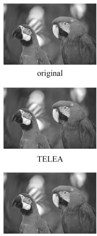
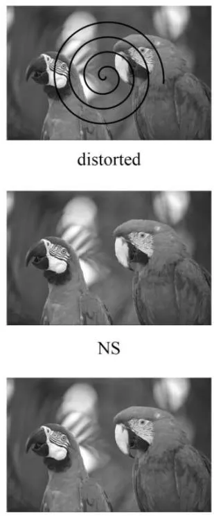
Fig. 14: Monochromatic image inpainting sample results

f) Discussions

Summing up our observations and results for the Kodak image dataset and other specific cases, we can say that the TELEA inpainting algorithm is the most efficient algorithm if runtime is a constraint i.e. the user needs to perform the inpainting operation as fast as he can and produce the best results. On the other hand, FSR_BEST inpainting algorithm is the most efficient algorithm if runtime is not a constraint i.e. the user has no time limit for the inpainting operation and wants to get the best result. The average memory consumption for all the inpainting algorithms are modest, hence memory will hardly be an issue in any system while running the Open CV inpainting algorithms.

	With runtime as a constraint	Without runtime as a constraint
Most effective OpenCV inpainting algorithm	TELEA algorithm	FSR_BEST algorithm

VI. FUTURE SCOPE

Our inpainting comparison study was done on the Kodak image dataset, a relatively small dataset containing 25 images only. The study can be done on a larger, more robust dataset which contains variety of images. This can be done to get more extensive results. We compared our results on the basis of four metrics only; more intricate metrics may be defined for the testing. Our study can be a base for analysing how various OpenCV inpainting methods work on images with different colour profiles.

We ran tests using four custom error masks. The error masks considered were mostly linear in shape. Other type of error masks such as curved, mixture of linear and curved can be taken for testing. This study can be a base for a comprehensive study on video inpainting techniques, which would be beneficial for people looking to work in this field.

VII. CONCLUSION

In conclusion, we present a comparative study of the various OpenCV inpainting algorithms, focusing extensively on their practical uses. The purpose of this paper is to apprise new users and researchers of the most efficient inpainting algorithm provided by OpenCV:TELEA algorithm for time constrained operations and FSR_BEST algorithm for non time constrained operations. We present the most efficient OpenCV inpainting algorithm to be used for various scenarios, which can help a beginner at inpainting to make his decision wisely without any further research. This study can be a base for more detailed comparative works on image and video inpainting. Inpainting is an evolving domain of image processing with major strides being made in the past, and much more sophisticated algorithms yet to arrive. It opens up the doorway for new image processing researchers to better the existing algorithms and create finer advanced inpainting algorithms which achieve near perfect accuracy.