## I. INTRODUCTION WHEN working with several aggregated services in a telecommunications network, we must resort to a digital network of integrated services. Integration means that the network can carry many types of information, such as voice, video, and data, all in digital form, using a single infrastructure. The general problem in a multiplexing system is that resources are shared by a set of heterogeneous sources. Multiplexing poses a mathematical and statistical problem: estimating the resource requirements of a font or set of fonts and, as sources are variable, statistical gain is to be expected. The different requirements of each service during the connection can be explored by statistical multiplexing. Since the notion of Effective Bandwidth (EB) introduced by Kelly in 1996 [4], the development of statistical tools that allow finding expressions to estimate the probability of loss in a link has emerged strongly. The problem with multiplexing is that the probability of many sources deciding to dispatch the maximum rate, in which case there would be an overflow, is not zero. Admission control mechanisms must be in place to accept a new connection, which minimizes the effects of data loss while maintaining the quality of service (QoS) for both current and future sources. Therefore, it will be essential to have mathematical models that describe the behavior of the sources. Traffic modelingin network services is necessary in order to dimension their components and evaluate their performance. Traffic models can be used both to find the appropriate descriptors that characterize the service, and facilitate management tasks, such as the establishing of control admission criteria (CAC). In particular, we are interested in applying estimation techniques from the traffic traces of a data network to monitor and predict network performance so that more opportune and effective control decisions can be made. This paper is structured as follows: Section II introduces the Generalized Markov Fluid Model and provides an expression to determine the EB for this model. This tool is used to measure the channel occupancy of each source. Section III studies the kernel estimation techniques and the Gaussian mixture model, to use these tools to estimate the EB for our model. Section IV presents the parameters of the simulated model and the estimation methods of the EB of the GMFM from traces. A comparison of the estimation methods is presented in section V, and conclusions are drawn in Section VI, along with some considerations for future work. ## II. TRAFFIC DESCRIPTION ### a) The Model Modulated Markovian models have been developed for more than two decades. They have been especially useful for modeling, with relative accuracy, many real data sources because they can capture the temporal correlation of the data. These processes are characterized by a set of states, which form a Markov chain, and the transition times. In this work, we use the Generalized Markov Fluid Model, introduced in [1], due to its properties. This model is modulated by a continuous-time, homogeneous and irreducible Markov chain. In each state of the chain, the generation rate is a random variable, distributed according to a probability law, depending on the state, that does not change during the time interval in which the Markov chain is in that state. The interpretation of the model is that each state in the chain is identified as the activity performed by a user, such as chatting or videoconferencing. Hence, a sudden change in transfer rate reports a change of state in the chain. Within a state, the data transfer rate assumes values that depend specifically on that activity, according to some probability distribution. ### b) The Effective Bandwidth Multiplexing variable rate sources on a link result in reserving for each source a capacity more significant than the average transmission rate, which would be a very optimistic measure, but less than the maximum transmission rate, which would be a pessimistic measure and lead to a waste of resources. For this purpose, the EB defined by F. Kelly in [4] is a valuable and realistic measure of channel occupancy. To estimate EB for a given GMFM from traffic traces, formulas of the type obtained by Kesidis, Walrand, and Chang [5] were obtained. Let us consider $\{X_{t}\}, t \geq 0$ a GMFM. Then the effective bandwidth has the following expression $$ \alpha (s,t) = \frac{1}{s t} \log \left\{\pi \exp \left[ (Q + s H) t \right] \mathbf{1} \right\}, $$ where 1 is a column vector with all entries equal to $1$, $\pi$ and $Q$ are the invariant distribution and the infinitesimal generator for the modulating chain, respectively. $H$ is a diagonal matrix whose dimension is equal to the number of states of the chain and whose non-zero elements are the first moments, $\mu_{i}$, of the law governing the generation rate in state i. This expression provides a way to estimate the EB from traffic traces. Estimators of the infinitesimal generator of the modulator chain, its invariant distribution, and the average transfer rate, and their properties can be found in [1]. ## III. ESTIMATION METHODS In this section, the estimators $\hat{\mathbf{Q}},\hat{\mathbf{H}},$ and $\hat{\pi}$ of the parameters involved in (1) are calculated using different techniques. ### a) Kernel Density Estimation One of the most common methods for nonparametric estimation of a density is the well-known kernel estimator. Given a simple random sample $X_{1}, \ldots, X_{n}$ of the random variable of interest $X$ with density $f$, the expression of the estimator is $$ \hat {f} (x) = \frac {1}{n h} \sum_ {i = 1} ^ {n} K \left(\frac {x - X _ {i}}{h}\right), \tag {2} $$ where $h > 0$ is a smoothing parameter, and $K$ is the kernel function which is non-negative, bounded, real-valued, unimodal, symmetric around 0, and its integration is 1. It is possible to choose different types of functions for the K-kernel. We choose to work with Gaussian kernels. The smoothing parameter $h$ must tends slowly to zero; this means that $h \to 0$, $nh \to \infty$, to ensure that $\hat{f}$ tends to the true density $f$. The window size parameter $h$ is an essential aspect of these techniques, as seen in [3]. Density estimation will be smoother the larger the window. The peaks are associated with the states of the chain, if they are close together, a "large" h could lead to merging close peaks and drawing incorrect conclusions, but a "small" h could show too many peaks leading to spurious maxima. The invariant distribution of the modulate chain was calculated using a suitable window size in (2). With the number of peaks, we estimate the number of states of the chain, because it is a multimodal density. The values where the maxima are reached represent the average sending rate in each state. We estimate the range of dispatch values associated with each state, with the values of the minima adjacent to each maximum. Next, with the area under the density, within each range, we estimate the probability $\pi_{i}$ of each state $i$. Thus, $\pi$ can be reconstructed because both spatial and temporal behavior converge at the GMFM, as seen in [3]. ### b) Gaussian Mixture Model In the statistical context, we can define a mixture model as a probabilistic model to represent the incidence of subpopulations within the same population. For this reason, they are helpful for estimating the invariant probability of the modulate chain and the average dispatch rates in each state. As the Gaussian distribution is fitted to model the distribution of the dispatch rate in each case, we will use Gaussian Mixture Models (GMM). These models are an example of a parametric probability density function which can be represented as a weighted sum of all Gaussian component densities. Let us assume that there are $k$ clusters. Equation that defines a Gaussian Mixture is $$ \pi (x) = \sum_ {i = 1} ^ {k} \pi_ {i} N (x | \mu_ {i}, \Sigma_ {i}). $$ Each Gaussian explains the data contained in every single cluster, and the mixing coefficients are themselves probabilities and must satisfy the following condition $$ \sum_ {i = 1} ^ {k} \pi_ {i} = 1. $$ To determine the optimal values for these, we need to establish the maximum likelihood of the model. A general technique for finding maximum likelihood estimators in these models is the Expectation-Maximization, or simply the EM algorithm. This is widely used for optimization problems where the objective function has complexities, such as the one we have just found for the GMM case. To apply this iterative process, we must initialize the parameters of our model $\theta = \{\pi, \mu, \Sigma\}$, with some value. In our case, we use the results obtained by a previous K-Means algorithm as a good starting point for our algorithm. EM algorithm consists of two steps; the first one finds an expression for the expected value of the log-likelihood, given the initial valuesor the prior estimation of the parameters, and the second step maximizes that expectation over the parameter space. More details about these algorithms are discussed in [2] and [6]. ## IV. 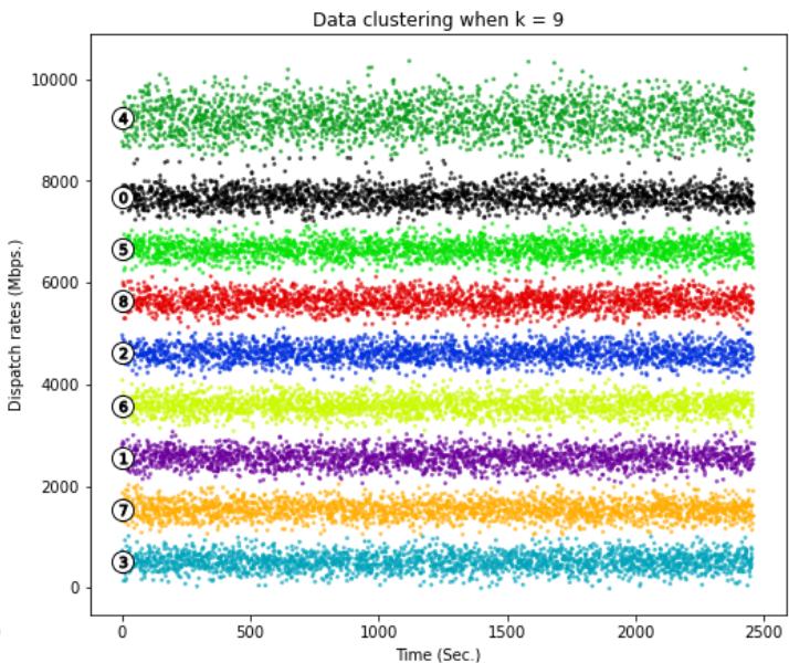SIMULATION AND NUMERICAL RESULTS In this section, we will perform the analysis using simulated traffic traces generated by simulations to estimate with both methods. Simulations were performed in Python 3.7 using sklearn.neighborslibrary, [7] and codes can be provided by asking the authors. Several traffic simulations were performed according to the presented model presented in (II-A), where the modulating Markov chain has $k = 9$ states, and each state is associated with a data transfer rate interval shown in the table below. To design the infinitesimal chain generator, we consider that the chain can pass from one state to another, with the same probability. Even it is not a very realistic model, we believe that it is the most adequate for comparing different estimation methods, so <table><tr><td>State</td><td>Transfer speed (Mbps)</td></tr><tr><td>1</td><td>(0,1024]</td></tr><tr><td>2</td><td>(1024,2048]</td></tr><tr><td>3</td><td>(2048,3072]</td></tr><tr><td>4</td><td>(3072,4096]</td></tr><tr><td>5</td><td>(4096,5120]</td></tr><tr><td>6</td><td>(5120,6144]</td></tr><tr><td>7</td><td>(6144,7168]</td></tr><tr><td>8</td><td>(7168,8292]</td></tr><tr><td>9</td><td>(8292,10240]</td></tr></table> $$ Q = \left( \begin{array}{c c c c c c c c c} - 8 & 1 & 1 & 1 & 1 & 1 & 1 & 1 & 1 \\1 & - 8 & 1 & 1 & 1 & 1 & 1 & 1 & 1 \\1 & 1 & - 8 & 1 & 1 & 1 & 1 & 1 & 1 \\1 & 1 & 1 & - 8 & 1 & 1 & 1 & 1 & 1 \\1 & 1 & 1 & 1 & - 8 & 1 & 1 & 1 & 1 \\1 & 1 & 1 & 1 & 1 & - 8 & 1 & 1 & 1 \\1 & 1 & 1 & 1 & 1 & 1 & - 8 & 1 & 1 \\1 & 1 & 1 & 1 & 1 & 1 & 1 & - 8 & 1 \\1 & 1 & 1 & 1 & 1 & 1 & 1 & - 8 \end{array} \right). $$ Within each of these intervals, the amount actually dispatched comes from a Gaussian probability distribution. The simulated trace is a succession of pairs $(v_{i} t_{i})$ with $i$ from 0 to 20000, where $v_{i}$ is the transfer speed, $t_{i}$ is themoment when the chain jumps to another state, and 20000 is the number of jumps in the chain, so the link transfers at the speed $v_{i}$ while $t_{i-1} < t < t_{i}$. ### a) Determining the optimal number of clusters: Silhouette method Many clustering techniques are based on a first estimation as a starting point, which requires prior knowledge of the number of clusters. The Silhouette coefficient, a popular method of measuring the clustering quality, which combines both cohesion and separation [8], is rather independent of the number of clusters, k. For object $x_{i}$, the silhouette coefficient is expressed as follows: $$ s_{x_i} = \frac{b_{x_i} - a_{x_i}}{\operatorname{max}(a_{x_i}, b_{x_i})}, $$ where $a_{x_i}$ is the average distance of object $x_i$ to all other objects in its cluster; for object $x_i$ and any cluster not containing it, calculate the average distance of the object to all the objects in the given cluster, and $b_{x_i}$ is the minimum of such values for all clusters. It is possible to obtain an overall measure of the goodness of clustering by calculating the average silhouette coefficient of all objects. For one clustering with $k$ categories, the average silhouette coefficient of the cluster is taking the average of the silhouette coefficients of objects belonging to the clusters; that is: $$ \bar{s}_{k} = \sum_{i=1}^{n} s_{x_{i}} $$ where $n$ is the total number of objects in the data set. Value of the silhouette coefficient can vary between -1 and 1. Higher value indicates better clustering quality. The sum of squared errors (SSE) and the silhouette coefficient are combined to measure the quality of clustering and determine the optimal clustering number, $k_{\mathrm{opt}}$. Data objects in the same cluster are similar, and objects from distinct clusters are different from each other. This distribution minimizes the SSE of each data object from its cluster center. SSE is a commonly used criterion in measuring the quality of clustering; lower SSE indicates better partition quality for partitions with the same k. This criterion is defined as follows: $$ S S E = \sum_ {i = 1} ^ {k} \sum_ {x _ {j} \in C _ {i}} \| x _ {j} - c _ {i} \| ^ {2}, $$ where $x_{j}$ is the $j$ -th object in cluster $C_{i}$, and $c_{i}$ is the center of cluster $C_{i}$. To determine the optimal clustering number, we introduce the silhouette coefficient to work in conjunction with the SSE criterion because the SSE criterion is sensitive to the number of clusters, $k$. In this paper, we conduct a k-means clustering analysis of the dispatch rates under different k values. We plot the curves of the SSE and average silhouette coefficient against the number of clusters to analyze the two curves and identify the optimal number of clusters, $k_{opt}$. Below we show comparative results on the k-data clustering configuration from 7 to 11.  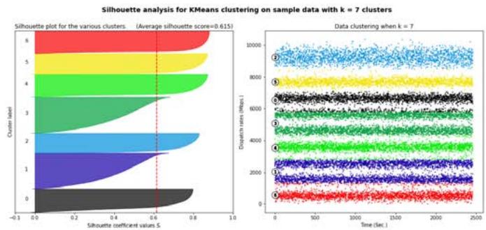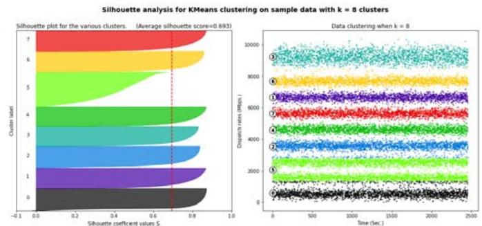 Fig. 1: Silhouette analysis for $k = 7$ and $k = 8$. Figure 1 and Figure 3 show that choices of $k$ equal to 7, 8, 10 or 11 would not be appropriate due to the presence of groups with below-average silhouette scores and wide fluctuations in the size of the silhouette plots. The value of $k = 9$ looks to be optimal one, as shown in Figure 2. The silhouette score for each cluster is above average silhouette scores. In addition, the thickness of the silhouette, plot representing each cluster is similar.  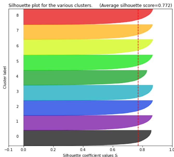Silhouette analysis for KMeans clustering on sample data with $k = 9$ clusters  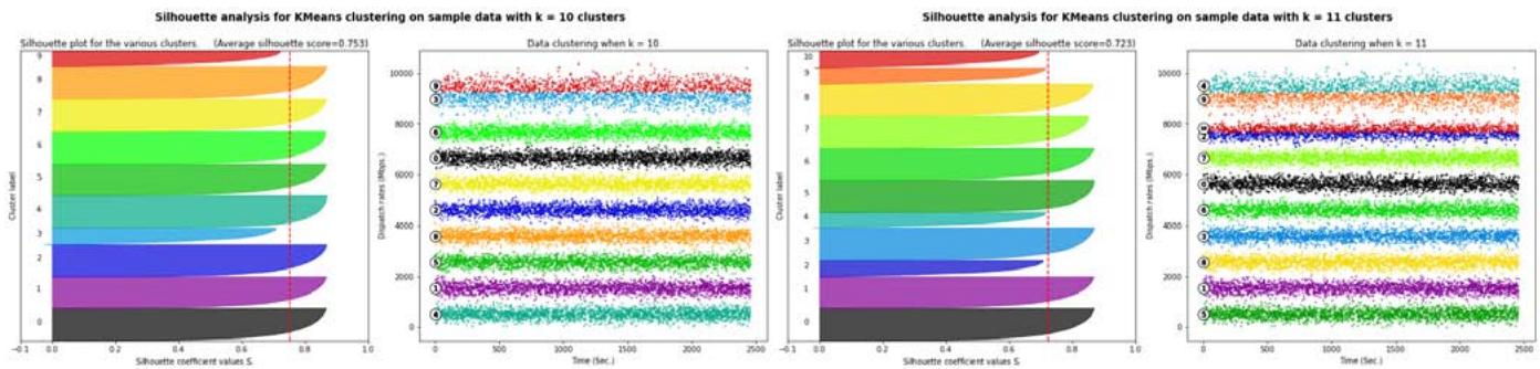 Fig. 2: Silhouette analysis for $k = 9$. Finally, we plotted the curves of the SSE and average silhouette coefficient against the number of clusters to analyze the two curves to determine the optimal number of clusters, $k_{\mathrm{opt}}$. 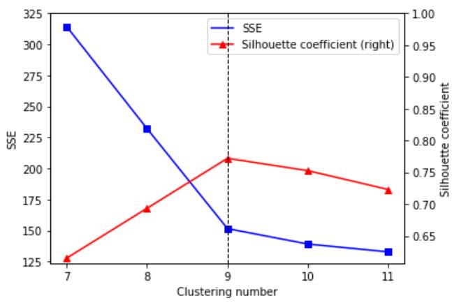 Fig. 4: SSE and average silhouette coefficient versus the number of clusters. Figure 4 draws a curve of scores, one score, Silhouette coefficient, for each alternative number of clusters. Elbow marks the point where the line exhibits its maximum curvature. Let us note that, before reaching this point, an increase in the number of clusters helps to reduce the sum of squared errors SSE. It is to be expected that behind the elbow, we find diminishing returns: incremental reductions of the SSE, by adding more clusters, would become more negligible the farther we go beyond the elbow and would do so relatively faster after having passed the inflection point of the curve: its elbow. This value is reached when the data are grouped into 9 clusters, so we conclude from this analysis that the optimal number of clusters is $k_{\mathrm{opt}} = 9$. ### b) Estimations from Traces We categorize the dispatch rates according to the clustering result with $k_{\mathrm{opt}} = 9$ as the clustering number. We consider that within each interval, the dispatched comes from a Gaussian distribution centered to its midpoint and deviation equal to one sixth of the length of the interval. ## i. Kernel Estimation Method For the simulated trace, we estimated the EB through the following steps: 1. Apply a Gaussian kernel to all $v_{i}, 0 \leq v_{i} \leq 20000$, with $h = 200$, to obtain $\hat{\pi}(x)$ for $0 < x < 10240$. This is possible because GMFM is ergodic, and time and spaces averages converge. See Figure 5. 2. Find minima for $\hat{\pi} (x)$. These minima are an estimate for the extremes of the dispatch ranges, which in turn allow us to determine the state of the modulating chain. As Gaussian distribution is symmetric, we determine rate averages using the estimated rank middle points. Finally, area under $\hat{\pi} (x)$ between two consecutive minima estimates $\hat{\pi}_i$. 3. Go through the trace comparing each $v_{i}$ with the rank estimated to assign the corresponding state, to obtain the estimated chain $(\hat{c}_i,t_i)$, $0\leq i\leq 20000$. 4. Estimate infinitesimal generator from $(\hat{c}_i, t_i)$ where $t_i$ are cumulative so first order difference of $t_i$ gives permanence time in state $c_i$. 5. Calculate the estimated EB with $\widehat{H},\widehat{\pi}$,and $\widehat{Q}_i$ as in (1). We chose the window width of 200 as it provides a reasonable estimate at a low computational cost. Figure 5 shows the theoretical and estimated density. 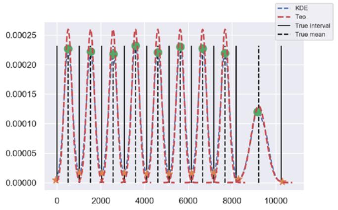 Fig. 5: Theoretical and estimated density, using Kernel Estimation techniques. The estimation of the infinitesimal generator is as follows. $$ \hat{Q} = \left( \begin{array}{cccccccc} -8.2507 & 0.9618 & 1.0355 & 1.0650 & 1.0355 & 1.0723 & 0.8991 & 1.0355 & 1.1350 \\0.9603 & -7.9626 & 0.8585 & 1.0331 & 0.9385 & 1.0403 & 1.1204 & 1.0585 & 0.9458 \\1.0164 & 0.8857 & -7.8808 & 1.0527 & 1.0999 & 0.9184 & 0.9983 & 0.8785 & 1.0309 \\1.0265 & 1.1078 & 1.0302 & -8.3599 & 0.9601 & 1.0782 & 1.0339 & 1.0154 & 1.004 \\1.0004 & 0.9279 & 1.0185 & 1.0149 & -7.9377 & 1.0620 & 1.0366 & 0.9786 & 0.8989 \\1.0654 & 1.0474 & 1.0403 & 1.0259 & 0.9506 & -8.0746 & 0.9649 & 1.0726 & 0.8860 \\0.9801 & 1.0532 & 0.9654 & 1.0569 & 1.0642 & 1.0459 & -8.2244 & 1.0678 & 0.9874 \\1.0078 & 1.0448 & 1.0078 & 1.0411 & 1.0115 & 1.0226 & 1.1518 & -8.3248 & 1.0115 \\1.1135 & 0.9761 & 0.9947 & 0.9761 & 0.9576 & 0.9910 & 1.0170 & 1.1060 & -8.1320 \end{array} \right) $$ The heat map in Figure 6 shows the percentage estimation error of the infinitesimal generator, obtained as the difference between each element with its estimate. Negative values in the heat map indicate an underestimation, and positive values an overestimating the infinitesimal generator elements. 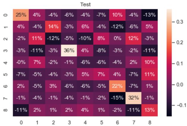 Fig. 6: Heat map for infinitesimal generator estimation errors. We use the confusion matrix $M$ to evaluate the performance in state estimation. $$ M = \left( \begin{array}{c c c c c c c c} 2235 & 3 & 0 & 0 & 0 & 0 & 0 & 0 \\4 & 2182 & 4 & 0 & 0 & 0 & 0 & 0 \\0 & 4 & 2167 & 4 & 0 & 0 & 0 & 0 \\0 & 0 & 1 & 2257 & 3 & 0 & 0 & 0 \\0 & 0 & 0 & 4 & 2184 & 8 & 0 & 0 \\0 & 0 & 0 & 0 & 2 & 2240 & 3 & 0 \\0 & 0 & 0 & 0 & 0 & 3 & 2243 & 6 \\0 & 0 & 0 & 0 & 0 & 0 & 2 & 2236 & 0 \\0 & 0 & 0 & 0 & 0 & 0 & 0 & 5 & 2200 \end{array} \right). $$ Rows are the actual states, and columns are the predicted or estimated states. For example, the 4 in matrix M at row 3, column 2 indicates that four times the chain was in state 3 but was estimated to be in state 2. ## ii. Gaussian Mixture Model Through the following steps, we estimate the EB for the simulated trace. 1. Apply GMM to all $v_{i}, 0 \leq v_{i} \leq 20000$ and obtain the means $\mu_{j}$, which will be the centers of each of the 9 clusters, the variances $\sigma_{j}^{2}$, and the weights of the mixture, $\pi_{j}, 1 \leq j \leq 9$. 2. Reconstruct the dispatch rate intervals, using $99\%$ of the area of each Gaussian distribution, centered at $\mu_{j}$ and with $\sigma_{j}^{2}$ variance, $1 \leq j \leq 9$. The value 0 is token as the lower limit of the first interval. 3. Go through the trace comparing each $v_{i}$ with the rank estimated to assign the corresponding state, to obtain the estimated chain $(\hat{c}_i,t_i)$, $0\leq i\leq 20000$. 4. Estimate infinitesimal generator from $(\hat{c}_i, t_i)$ where $t_i$ are cumulative so first order difference of $t_i$ gives permanence time in state $c_i$. 5. Calculate the estimated EB with $\widehat{H},\widehat{\pi}$, and $\hat{Q}$ as in (1). Figure 7 shows the theoretical and estimated density. In this case, the estimation of the infinitesimal generator is as follows. $$ \hat {Q} = \left( \begin{array}{c c c c c c c c c} - 8. 2 3 9 7 & 0. 9 6 1 8 & 1. 0 3 9 2 & 1. 0 6 1 3 & 1. 0 3 5 5 & 1. 0 7 2 3 & 0. 8 9 9 1 & 1. 0 3 1 8 & 1. 1 3 8 7 \\0. 9 6 0 3 & - 7. 9 5 5 3 & 0. 8 5 8 5 & 1. 0 2 9 4 & 0. 9 4 2 1 & 1. 0 4 0 3 & 1. 1 1 3 1 & 1. 0 6 2 2 & 0. 9 4 9 4 \\1. 0 1 5 5 & 0. 8 8 4 9 & - 7. 8 6 9 9 & 1. 0 4 8 1 & 1. 0 9 8 9 & 0. 9 1 7 6 & 0. 9 9 7 3 & 0. 8 6 6 8 & 1. 0 4 0 9 \\1. 0 2 7 5 & 1. 1 0 8 8 & 1. 0 2 3 8 & - 8. 3 5 6 8 & 0. 9 6 1 0 & 1. 0 7 9 2 & 1. 0 3 1 2 & 1. 0 1 6 4 & 1. 1 0 8 8 \\1. \mathbf {0} \mathbf {0} \mathbf {0} \mathbf {4} \mathbf {4} \mathbf {7} \mathbf {9} \mathbf {7} \mathbf {9} \mathbf {9} \mathbf {9} \mathbf {9} \mathbf {9} \mathbf {9} \mathbf {9} \mathbf {9} \mathbf {9} \mathbf {9} \mathbf {9} \mathbf {9} \mathbf {9} \mathbf {9} \mathbf {9} \end{array} \right). $$ 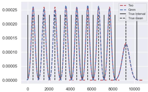 Fig. 7: Theoretical and estimated density, using Kernel Estimation techniques To evaluate the performance of the estimator, we show in Figure 8 the heat map for the estimation error of the infinitesimal generator. 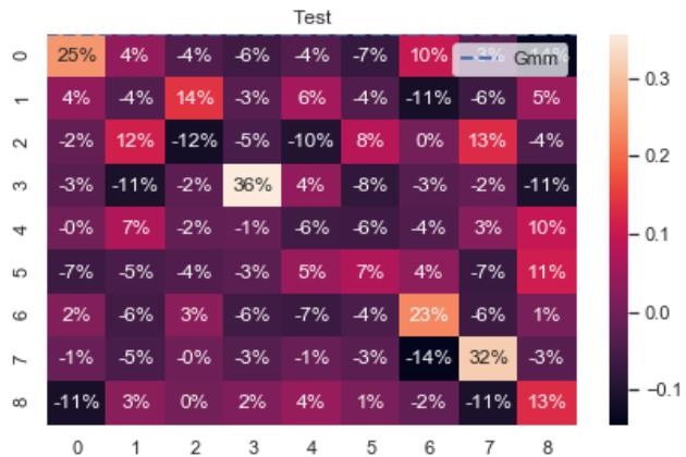 Fig. 8: Heat map for infinitesimal generator estimation errors. The confusion matrix M that we show below allows us to evaluate the performance in the estimation of the states. $$ M = \left( \begin{array}{c c c c c c c c} 2235 & 3 & 0 & 0 & 0 & 0 & 0 & 0 \\4 & 2182 & 4 & 0 & 0 & 0 & 0 & 0 \\0 & 4 & 2167 & 4 & 0 & 0 & 0 & 0 \\0 & 0 & 3 & 2254 & 4 & 0 & 0 & 0 \\0 & 0 & 0 & 3 & 2185 & 8 & 0 & 0 \\0 & 0 & 0 & 0 & 2 & 2240 & 3 & 0 \\0 & 0 & 0 & 0 & 0 & 3 & 2241 & 8 \\0 & 0 & 0 & 0 & 0 & 0 & 2 & 2236 \\0 & 0 & 0 & 0 & 0 & 0 & 0 & 2203 \end{array} \right). $$ ## V. COMPARISON OF THE RESULTS OBTAINED To compare both methods, in this section, we present the theoretical parameters and their respective estimates. Table I shows the estimated values of the average dispatch rates in each method and the value with which the traces were simulated, and the same is done for the class ranges of dispatch in Table II. Both methods allow for to reconstruct of the modulate chain very well, and this can be seen in their confusion matrices. However, in the EB estimation, the Gaussian Mixture Model is more efficient, as can be seen in Figure 9 and zoom of it in Figure 10. Table I: Theoretical and estimated ranges of dispatch. Theoretical range Estimated range <table><tr><td rowspan="2">Theoretical range</td><td colspan="2">Estimated range</td></tr><tr><td>KDE</td><td>GMM</td></tr><tr><td>0</td><td>0</td><td>0</td></tr><tr><td>1024</td><td>1026.1086</td><td>1024.1057</td></tr><tr><td>2048</td><td>2047.0149</td><td>2044.5478</td></tr><tr><td>3072</td><td>3069.9408</td><td>3078.4938</td></tr><tr><td>4096</td><td>4099.5986</td><td>4098.4828</td></tr><tr><td>5120</td><td>5121.1781</td><td>5124.6486</td></tr><tr><td>6144</td><td>6143.7674</td><td>6140.8196</td></tr><tr><td>7168</td><td>7163.6639</td><td>7156.2757</td></tr><tr><td>8192</td><td>8360.9483</td><td>8189.6392</td></tr><tr><td>10240</td><td>10240.0000</td><td>10240.0000</td></tr></table> Table II: Theoretical and estimated average dispatch rates. <table><tr><td rowspan="2">Theoretical range</td><td colspan="2">Estimated range</td></tr><tr><td>KDE</td><td>GMM</td></tr><tr><td>512</td><td>513.8042</td><td>513.2390</td></tr><tr><td>1536</td><td>1535.7202</td><td>1535.4954</td></tr><tr><td>2560</td><td>2561.3389</td><td>2559.7032</td></tr><tr><td>3584</td><td>3585.6112</td><td>3585.3959</td></tr><tr><td>4608</td><td>4609.2103</td><td>4611.1025</td></tr><tr><td>5632</td><td>5633.8191</td><td>5634.6542</td></tr><tr><td>6656</td><td>6654.0522</td><td>6653.1858</td></tr><tr><td>7680</td><td>7676.3049</td><td>7676.4876</td></tr><tr><td>9216</td><td>9209.5156</td><td>9223.2794</td></tr></table> 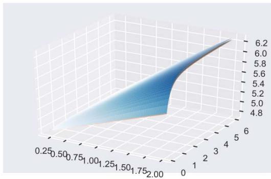 Fig. 3: Silhouette analysis for $k = 10$ and $k = 11$. 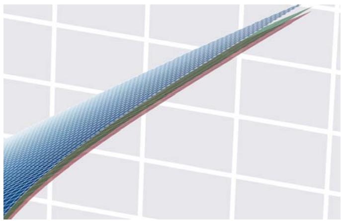 Fig. 9: Theoretical bandwidth (blue), bandwidth estimation using KDE (red) and mixed Gaussian (green). Fig. 10: Figure 9 zoom. ## VI. CONCLUSION In this paper we have proposed two methods to estimate effective bandwidths from traffic traces of a GMFM source. Numerical examples of simulated traces were presented showing the results obtained. Estimation process worked much better in the Gaussian Mixture model, as seen in the graphics presented. It is expected to extend the statistical calculation using an infinitesimal generator that models a more realistic behavior of the source and also in which the supports of each probability law have a greater intersection to develop the estimation to real data scenarios.

Generating HTML Viewer...

References

8 Cites in Article
José Bavio,Beatriz Marrón (2018). Properties of the Estimators for the Effective Bandwidth in a Generalized Markov Fluid Model.
C Bishop (2006). Pattern Recognition and Machine Learning.
R Coudret,G Durrieu,J Saracco (2013). Comparison of kernel density estimators with assumption on number of modes.
Frank Kelly (1996). Notes on effective bandwidths.
G Kesidis,J Walrand,C-S Chang (1993). Effective bandwidths for multiclass Markov fluids and other ATM sources.
K Murphy (2012). Machine Learning: A Probabilistic Perspective.
F Pedregosa (2011). Getting Started with Scikit‐learn for Machine Learning.
P Tan,M Steinbach,V Kumar (2006). Introduction to Data Mining.
No ethics committee approval was required for this article type.
Data Availability
Not applicable for this article.
How to Cite This Article
José Bavio. 2026. \u201cComparison of Effective Bandwidth Estimation Methods for Data Networks\u201d. Global Journal of Computer Science and Technology - E: Network, Web & Security GJCST-E Volume 22 (GJCST Volume 22 Issue E2).
Explore published articles in an immersive Augmented Reality environment. Our platform converts research papers into interactive 3D books, allowing readers to view and interact with content using AR and VR compatible devices.
Your published article is automatically converted into a realistic 3D book. Flip through pages and read research papers in a more engaging and interactive format.
Our website is actively being updated, and changes may occur frequently. Please clear your browser cache if needed. For feedback or error reporting, please email [email protected]
Thank you for connecting with us. We will respond to you shortly.