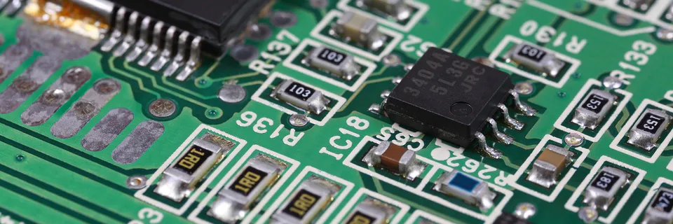
## I. INTRODUCTION The mother board assembly constitutes morphologically the brain of an engineering device. The integrated circuits that are photolithographically etched onto silicon chips constitutes morphologically the brain cells. However, the brain cells on individual silicon chip are isolated from other chips; and they need to be electrically interconnected. The brain cells are very delicate and even the interconnects are mechanically fragile; and they need to be mechanically protected. Lastly, the brain cells generate high intensity of heat when running, and the heat needs to be dissipated before the brain cells would be burned. The jobs of electrical interconnection, mechanical protection, and thermal dissipation rest on the design and engineering of electronic and microelectronic assemblies [1].  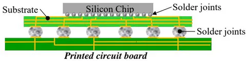Figure 1: Schematic of the Cross-Section of an IC Component and a PCB Figure 1 shows the schematic of a silicon chip that is electrically interconnected to a substrate, which is in turn interconnected to a printed circuit board, through arrays of solder joints. The former assembly is frequently referred to as an integrated circuit component/assembly while the latter is frequently referred to as a printed circuit board assembly. We shall refer to both assemblies as simply electronic assemblies. The solder joints are formed by melting solder balls/paste to form metallurgical bonds with the metal pads on the chip and the substrate, and with the metal pads on the substrate and the printed circuit board. Electronic assemblies are susceptible to undue stress during manufacturing and while in service resulting in functional failure. In general, electronic assemblies may experience three main physics of damage: the violent vaporisation of the ingress moisture in the integrated circuit assembly during the solder joint forming process leading to cracking and/or delamination of the assembly [2][3]; fracturing of interconnection caused by drop-shock of mobile electronic products [2][4]; and lastly, creep-fatigue damage of interconnecting solder joints after repeated cycles of powering on/off of engineering devices [2][5]. The last is especially critical and has attracted maximum interest in electronic assemblies. In essence, the differential thermal expansions between the silicon chip and the substrate and between the integrated circuit assembly and the printed circuit board give rise to cyclical deformation of the solder joints at temperature above their homologous temperature, driving them towards failure by the mechanism of creep fatigue. The propensity for creep fatigue failure of solder joints is aggravated by the trend towards increasing functionality of consumer electronic products, which is driving increase size of integrated circuit assembly and reduce size of solder joints. The failure of a nuclear plant or a commercial aircraft is accompanied by unacceptable catastrophic consequences. The structural integrity and reliability of such products are therefore the paramount design considerations. In contrast, the two paramount design considerations for electronic assemblies are electrical performance and space. The former to support the ever-increasing performance of electronic products and the latter to support the increasing functionality of electronic products. Failure of consumer electronic products in service though annoying is acceptable to most users. This has encouraged a relatively relax attitude towards the structural integrity of electronic assemblies; and this is further encouraged by the relatively short life cycle of consumer electronic products. Nevertheless, there is a positive aspect of this more relax attitude towards structural analysis. The structural design of electronic assemblies is not bounded by a design protocol or a design code. Electronic assembly engineers are free to use any analysis method so long as the designed electronic assemblies will meet the integrity and reliability test requirements. It is inherently easy to monitor the structural integrity of an electronic assembly through monitoring the electrical connectivity of the assembly [6]. If necessary, the growth of damage in an electronic assembly can be tracked in real time through monitoring the changing electrical impedance of the assembly [6][7]. The absence of a strict design protocol and the ease of validating an analysis with tests has encouraged the exploration and adoption of new analysis methods, notwithstanding some of these methods may not be robust. This manuscript gives a condensed presentation of the recent advances in the creep fatigue analysis of solder joints in electronic assemblies. This comprises two major analyses: thermomechanical analysis of solder joints in electronic assemblies; and creep fatigue life modelling of solder joints. It is believed that these advanced analyse techniques are fundamentally robust and they can be adopted to similar applications in other engineering field. ## II. THERMOMECHANICAL ANALYSIS OF SOLDER JOINTS Electronic assembly engineers routinely performed thermomechanical analysis of electronic assemblies using finite element analysis software in which the solder joints are modelled using solid finite elements. This has inadvertently led to singularity of stress/strain at discontinuities of geometry and materials giving rise to inconsistent analysis - because the magnitude of the stress/strain is dependent on the size and shape of the finite element at the site of singularity. To circumvent such singularity, electronic assembly engineers have adopted the practice of volume-averaging the stress/strain over a selected volume of solder joints [8][9]. Unfortunately, such arbitrary volume averaging act is equivalent to smearing the geometry of solder joints, effectively denying the engineers the ability to analyse the geometrical effects of solder joints on the magnitude of stress/strain. The issue of stress/strain singularity can be addressed by modeling the components of electronic assemblies as shells and beams. Maximum insights into the mechanics of the subject matter can be achieved through analytical modeling. 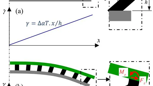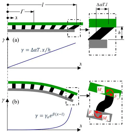Analytical models of varied sophistication have been reported in the electronic assembling community [10][11][12][13]. In essence, an electronic assembly is treated as a sandwich structure constituting of array of solder joints sandwiched between two outer members. The simplest model treats the outer members as being infinitely rigid and the solder joints as being infinitely compliant such that the solder joints experience only shear strain whose magnitude increases linearly with distance from the neutral plane of an electronic assembly and is given by $\gamma = \Delta \alpha T \cdot x / h$ (Figure 2a) [10], where $\Delta \alpha T$ is the differential thermal strain between the two outer members, $x$ is the distance of a discrete joint from the neutral plane of the assembly, and $h$ is the height of the discrete joint. This unrealistic model would grossly overestimate the magnitude of shear strain. The more sophisticated models treat the outer members as rectangular beams; and the solder joints as linear springs [11], or as cylindrical beams that are capable of shearing, flexing, and stretching [12][13]. The inclusion of elasticity of the outer members in the model have led to the vital understanding that shear strain in the solder joints does not increase linearly but exponentially with distance from the neutral plane of an electronic assembly. It takes the form $\gamma = \gamma_{o} e^{\beta (x - l)}$ (Figure 2b), where $\gamma_{o}$ is approximately the shear strain at the outmost solder joint, $\beta$ is a compliance parameter of the assembly, $l$ is the half-length of the assembly.  Figure 2: Analytical Models with Closed-Form Solution: (a) Infinitely Rigid Outer Members; (b) Outer Members as and Solder Joints as Elastic Beams ### a) Analytical Modelling Evaluating the stresses in the discrete joints of an assembly involves four steps of analysis, starting with smearing the discrete joints into a continuously bonded joint and then evaluating the compliances of the smeared assembly. This is followed by evaluating the smeared stresses in the smeared joints. The third step integrates the stresses into boundary forces and moments acting on individual discrete joint. The last step evaluates the stresses in the discrete joint due to the boundary forces and moments. The discrete joints are assumed to be of identical shape and size and are distributed at uniform spacing. Figure 3 shows the schematic of discrete joints with a height $h_d$ and spacing at pitches $p_x$ and $p_y$ along the $x$ and the $y$ coordinates, respectively. In the case that individual discrete joint is not of cylindrical shape but one with non-uniform sections along its height, it is represented by a pseudo cylindrical joints with a representative shear area, $A_{d,rep}$, and a representative second moment of area, $I_{d,rep}$, that would return identical shear and flexural stiffnesses as the original discrete joints [14]. 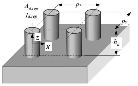Theses representative parameters are given by  Figure 3: Schematic of Solder Joints $$ A_{d,rep} = \frac{1}{\int_{-h_d/2}^{h_d/2} \frac{dz}{A_Z(z)}} \quad _{ep} = \frac{1}{12 \int_{-h_d/2}^{h_d/2} \int_{-h_d/2}^{z} \frac{\xi d\xi}{I_Z(\xi)} dz} $$ Referring to the outer members as member #1 and member #2, and the discrete joint as member $\#d$, the height, the stretch modulus, the shear modulus, and the flexural stiffness of member $\#i$ are denoted as $h_i$, $E_i$, $G_i$, and $D_i$, respectively; the shear and the in-plane stretch compliances of the assembly are denoted as $\kappa_s$ and $\lambda_x$ respectively. For ease of reference, we shall refer to the moduli of the smeared joints as smeared moduli and the compliances as smeared compliances. Those characteristics that are associated with the smeared joints will be marked with an asterisk. ### b) Compliances of a Smeared Assembly The in-plane stretch compliance of the assembly is a function of the outer members and, for the case of plane stress, is given by [12][13] $$ \lambda_ {x} = \sum_ {i = 1} ^ {2} \left(\frac {1}{E _ {i} h _ {i}} + \frac {h _ {i} {} ^ {2}}{4 D _ {i}}\right), \tag {2} $$ where in $D_{i} = E_{i}h_{i}^{3} / 12$ for plane stress. The smeared shear compliance of the assembly, $\kappa_{s}^{*}$, is given by [12][13] $$ \kappa_{s}^{*} = \sum_{i=1}^{2} \kappa_{si} + \kappa_{sd}^{*} + \kappa_{sd\varphi}, $$ where $\kappa_{si} = \frac{h_i}{8G_i},\kappa_{sd}^* = \frac{h_d}{G_d^*},\kappa_{sd}\varphi = \frac{h_d^3}{12D_d^*}.$ (4) wherein $\kappa_{si}$ is associated with the shear compliance of member #i; $\kappa_{sd}^*$ is associated with the shear deformation of the smeared joints; while $\kappa_{sd\varphi}$ is associated with the flexural deformation of the discrete joints - referring to Figure 2b. The smeared shear modulus, $G_{d}^{*}$, and the smeared flexural rigidity, $D_{d}^{*}$, are given by $G_{d}^{*} = G_{d}A_{d,rep} / (p_{x}p_{y})$ and $D_{d}^{*} = E_{d}I_{d,rep} / (p_{x}p_{y})$. ### c) Stresses in Smeared Joints The shear stress in the smeared joints along the bonded length of a balanced assembly is given by [12][13][15][16] $$ \tau^ {*} (x) = A _ {c} ^ {*} e ^ {\beta^ {*} (x - l)}, x > 0, \tag {5} $$ where $$ A _ {c} ^ {*} = \frac {\varepsilon_ {T}}{\sqrt {\lambda_ {x} \kappa_ {S} ^ {*}}}, \tag {6} $$ $\beta^{*} = \sqrt{\lambda_{x} / \kappa_{s}^{*}};\varepsilon_{I} = \Delta \alpha T$ is the differential thermal strain between the outer members. ### d) Sectional Force and Moment in a Discrete Joint The magnitude of the sectional shear force on a discrete joint that is at a distance $\Gamma$ from the mid plane of the assembly may be evaluated approximately as $$ F _ {\tau} (\Gamma) \approx \tau^ {*} (\Gamma) p _ {x} p _ {y}, \tag {7} $$ The sectional shear force does not vary along the height of the discrete joint. 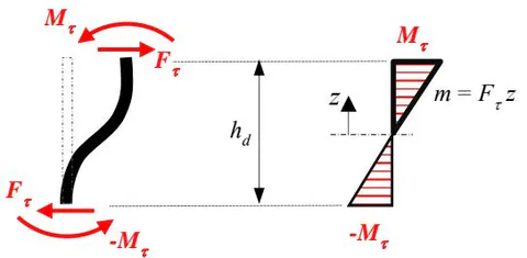On the other hand, and referring to Figure 4, rotational equilibrium dictates that the sectional moment varies linearly along the height of the discrete joint and is given by  Figure 4: Bending Moment Distribution Along a Discrete Joint $$ m (\Gamma , z) = F _ {\tau} (\Gamma) z, \tag {8} $$ where $z$ is the local coordinate of a solder joint as shown in Figure 3. ### e) Shearing and Bending Stresses in a Discrete Joint The distribution of shear stress and bending stress along the height of a discrete joint, assuming it being an Euler beam, are simply [12]\[13\]: $$ \tau_ {d} (\Gamma , z) = \frac {F _ {\tau} (\Gamma)}{A _ {d} (z)} \tag {9} $$ $$ \sigma_ {b} (\Gamma , z) = m _ {\tau} (\Gamma , z) \frac {r _ {d} (z)}{I _ {d} (z)} $$ where $A_{d}(z), I_{d}(z)$, and $r_d(z)$ are the local cross-sectional area, the local second moment of area, and the local outer fibre of the discrete joint. Assuming circular cross-section, as in the case of solder joints, the ratio $r_d / I_d$ is reduced to $4 / (\pi r_d^3)$. The largest magnitudes of shear force and bending moment, and hence shearing and the bending stresses, occur at the discrete joint furthest from the mid-plane of the assembly. Assuming $\Gamma_{\mathrm{max}} = l$, these stresses are given by $$ \tau_ {d, m a x} = \frac {F _ {\tau , m a x}}{A _ {d , m i n}} \tag {10} $$ $$ \sigma_ {b} (l, z) = \frac {4 F _ {\tau , m a x} z ^ {*}}{\pi r _ {d} ^ {3} (z)} $$ where $F_{\tau,max} = \frac{\varepsilon_Tp_xp_y}{\sqrt{\lambda_x\kappa_s^*}},$ (11) and $A_{d,\min}$ is the minimum cross-sectional area of the discrete joint. ### f) Optimum Shape of Solder Joints The solder joints are formed through controlled heating of solder into liquid form followed by controlled cooling the assembly to room temperature, forming metallurgical bonds with metal pads at its two ends. A solder joint will take up the natural shape of a spherical barrel, as shown in Figure 5a, that has the minimum surface energy. It is clear from Eq. (10) that a standard solder joint will experience the maximum magnitude of shear stress, $\tau_{d,max}$, and the maximum magnitude of bending stress, $\tau_{b,max}$, at its ends joining the outer members; and  Figure 5: Geometries of Solder Joints (a) Barrel Shape, (b) Flatten Barrel Shape, (c) Stout Hourglass $$ \frac {\sigma_ {b , m a x}}{\tau_ {d , m a x}} = \frac {2 h _ {d}}{r _ {d , e n d}} \tag {12} $$ where $r_{d, \text{end}}$ 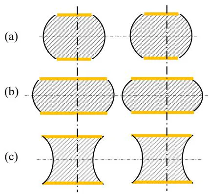is the radius of the solder joint joining the outer member. In a standard barrel-shape solder joint, the magnitude of $h_d$ is much larger than that of $r_{d, \text{end}}$. In other words, $\sigma_{b, \text{max}}$ is a far dominant stress in a standard barrel-shape solder joint. On paper, the magnitude of the dominant stress, $\sigma_{b, \text{max}}$, can be lowered by increasing the end radius of barrel-shape solder joints, which for the same volume of solder joint, will result in flatten barrel-shape solder joints leading to very significant reduction in the magnitude of $\sigma_{b, \text{max}}$. In practice, such a manipulation would inevitably raise the risk of bridging between adjacent solder joints, as is illustrated in Figure 5b. It is clear from the linear distribution of bending moment in solder joints, as depicted in Figure 4, that solder joints should ideally have the shape of an hourglass. Solder joints of progressive hourglass shape can be designed into electronic assembly [14]. Modeling the curvature of an hourglass-shape solder joint as a hyperbolic sine curve and evaluating its representative shear area, $A_{d,rep}$, and representative second moment of area, $I_{d,rep}$, using Eq. (1), a stout hourglass-shape solder joint – similar to that illustrated in Figure 5c – has been found to return the minimum magnitude of stress for the same volume of solder as a standard barrel-shape solder joint. The maximum magnitude of bending stress, $\sigma_{b,max}$, in the stout hourglass solder joints is less than $15\%$ that in a standard barrel-shape solder joints [14]. It is also worth noting that the use of stout hourglass solder joints does not increase the risk of bridging between solder joints. ## III. CREEP FATIGUE MODELING The fatigue life of a metal experiencing pure low cycle fatigue – that is, in the absence of aggravating element – and under a constant amplitude of cyclic stressing has been found to be satisfactorily modelled using the Coffin-Manson equation: $$ \varepsilon_ {p} = C _ {o} N _ {f} ^ {- \beta_ {o}}, \tag {13} $$ where $\varepsilon_{p}$ is the amplitude of the incremental plastic strain in a cycle; $N_{f}$ is the number of cycles to failure; $C_{o}$ and $\beta_{o}$ are material dependent fitting constants. While it is tempting to extend the equation to creep fatigue modelling by replacing the plastic strain amplitude, $\varepsilon_{p}$, with inelastic strain amplitude, $\varepsilon_{in} = \varepsilon_{p} + \varepsilon_{c}$, wherein $\varepsilon_{c}$ is the incremental creep strain in a single cycle, this simplicity approach of lumping creep strain with fatigue strain contradicts with the different macrostructural damages of creep and fatigue in metals [17][18] and has been convincingly disproved by abundant experimental data [19]. # a) A Brief Review of Practising Creep Fatigue Life Prediction Models The power generation community and the aerospace engineering community have vast knowledge and experience in modelling creep fatigue life of metals. Both the power generation and the aerospace communities have subscribed to the idea that creep fatigue damage can be evaluated by summing independently the damages due to creep, due to fatigue, and due to interaction of these two damages. The summative creep fatigue damage in a single creep fatigue cycle may be expressed mathematically as $$ d = d _ {f} + d _ {c} + d _ {c f}. \tag {14} $$ Interestingly, the two communities have subscribed to different idea of defining the respective damages, $d_{f}, d_{c}$, and $d_{cf}$. The aerospace community characterises the three cyclic damage indices from the hysteresis loop of a tension-compression creep fatigue experiment. Three components of inelastic strain: $\varepsilon_{pp}$, $\varepsilon_{cc}$, $\varepsilon_{cp}$ (or $\varepsilon_{pc}$ ) are partitioned and extracted from the hysteresis loop, wherein the first letter of the subscript ( $c$ for creep and $p$ for plastic strain) refers to the type of strain imposed in the tensile portion of the cycle, and the second letter refers to the type of strain imposed during the compressive portion of the cycle. Individual strain component is assumed to follow a power-law relation with the number of hysteresis cycles to failure. That is, $$ \varepsilon_ {j k} = C _ {j k} N _ {j k} ^ {- \beta_ {j k}}. \tag {15} $$ The damage per creep-fatigue cycle due to individual component is then simply $$ d _ {j k} = \frac {1}{N _ {j k}} = \left(\frac {\varepsilon_ {j k}}{C _ {j k}}\right) ^ {1 / \beta_ {j k}}. \tag {16} $$ This is known as the strain range partitioning model [19]. While this noble model has served the aerospace community well, its characterisation is inherently challenging. The power generation community conveniently treats the cyclic fatigue damage, $d_{f}$, as that due to pure fatigue, which can be evaluated using the Coffin-Manson equation; that is, $$ d _ {f} = \frac {1}{N _ {f}} = \left(\frac {\varepsilon_ {p}}{C _ {o}}\right) ^ {1 / \beta_ {o}}; \tag {17} $$ and the cyclic creep damage, $d_{c}$, as that due to pure creep, which may be evaluated using the creep strain exhaustion rule: $$ d _ {c} = \frac {1}{\varepsilon_ {R}} \int_ {0} ^ {t _ {c}} \dot {\varepsilon} _ {c} (t) d t, \tag {18} $$ wherein $\dot{\varepsilon}_c(t)$ is the instantaneous creep strain rate and $t_c$ the cyclic period. However, the cyclic creep-fatigue interaction damage, $d_{cf}$, is a fitting index, which can only be established through extensive experimental characterisation [20][21][22]. The electronic packaging professionals have fallen for the creep fatigue equation of Darveaux [9], $$ N_{cf} = K_1 w_{in}^{K_2} $$ where $w_{in} = w_p + w_c$ is the sum of the cumulative plastic work density and the cumulative creep work density in a single creep fatigue cycle. Just like the failed idea of substituting plastic strain with inelastic strain in Eq. (13), the act of lumping the two work densities is clearly against the macrostructural evidence of the two damages. Consequently, and unsurprisingly, the fitting constants, $K_1$ and $K_2$, are found to be dependent on the size and shape of individual electronic assembly [9], in other words, on the magnitude of the inelastic work density, $w_{in}$. Nevertheless, the electronic packaging community have stubbornly stuck with the model. ### b) Creep Integrated Fatigue Equation In the case of fatigue being the dominant mechanism in creep fatigue failure, the role of creep may be treated as one to lower the material capacity in fatigue. This has led to the idea of creep integrated fatigue equation [23][24]\[25\]: $$ \varepsilon_ {p} = C _ {o} c \left(\varepsilon_ {p}, T, t _ {c}\right) N _ {c f} ^ {- \beta_ {o}}; \tag {20} $$ where $c(\varepsilon_p, T, t_c)$ is a function. Expressing the fatigue capacity in Eq. (13) for the case of pure fatigue as $\varepsilon_{p,ref}$ and it becomes clear that $c\big(\varepsilon_p, T, t_c\big) = \varepsilon_p / \varepsilon_{p,ref}$ describes the fractional fatigue capacity of a subject in the presence of creep. Its magnitude ranges from zero to unity - a zero magnitude corresponds to the case of pure creep while a magnitude of unity corresponds to the case of pure fatigue. The function 1- $c(\varepsilon_p, T, t_c)$ describes the fractional creep damage acting on the subject. ## i. The Fundamental Equations of Pure Creep In Metals The strain rate in a uniaxial steady-stress creep rupture experiment may be described in the form of Sherby-Dorn equation, $\dot{\varepsilon}_{SD}$, or Larson-Miller equation, $\dot{\varepsilon}_{LM}$, or Manson-Haferd equation, $\dot{\varepsilon}_{MH}$: $$ \dot {\varepsilon} _ {S D} = f \left(\sigma_ {s}\right) e ^ {- H / k T}, T \geq 0 $$ $$ \dot{\varepsilon}_{LM} = B e^{-H(\sigma_s)/kT}, T\geq 0, \tag{21} $$ $$ \dot{\varepsilon}_{MH} = D e^{(T-T_{ref}) r(\sigma_{s})}, T\geq T_{ref} $$ wherein $f(\sigma_{s}), H(\sigma_{s})$, and $r(\sigma_{s})$ are functions of the applied tensile stress, $\sigma_{s}$; $k$ is the Boltzmann's constant; $H, B,$ and $D$ are material dependent constants; and $T_{ref}$ is the temperature below which the mechanism of creep is assumed to be dormant. Assuming the dominance of the secondary stage of creep, the eventual creep rupture strain, $\varepsilon_{R}$, is given by $$ \varepsilon_ {R} = \dot {\varepsilon} _ {I I} t _ {R}, \tag {22} $$ where $t_R$ is the time to creep rupture. Assuming $\varepsilon_R$ to be independent of the applied stress and temperature, Eq. (21) may be rearranged into: $$ P _ {S D} (\sigma_ {s}) = \frac {\varepsilon_ {R}}{f (\sigma_ {s})} = \frac {t _ {R}}{e ^ {H / k T}} $$ $$ P _ {L M} \left(\sigma_ {s}\right) = \frac {H \left(\sigma_ {s}\right)}{k} = \frac {\ln t _ {R} + \ln B _ {R}}{1 / T}, \tag {23} $$ $$ P _ {M H} (\sigma_ {s}) = - \frac {1}{r (\sigma_ {s})} = \frac {T - T _ {r e f}}{l n (t _ {R} / t _ {\infty})} $$ wherein $B_R = B / \varepsilon_R$ and $t_\infty = \varepsilon_R / D$. These functions are known respectively as the Sherby-Dorn parameter, the Larson-Miller parameter, and the Manson-Haferd parameter. These parameters describe the relations between the applied stress, $\sigma_s$, and the gradient of the respective time-temperature function. These relations can be readily characterized and are used extensively in the creep rupture design of metal structures. The corresponding stress parameter for a single stressing cycle may be expressed as \[25\]: $$ P _ {c \_ S D} (\sigma) = t _ {c} e ^ {- H / k T} $$ $$ P _ {c \_ L M} (\sigma) = T \left(\ln t _ {c} + \ln B _ {c}\right), \tag {24} $$ $$ P _ {c \_ M H} (\sigma) = \frac {T - T _ {r e f}}{l n (t _ {c} / t _ {c \infty})} $$ where $\sigma$ is the amplitude of the cyclic stress; and $B_{c} = B / \varepsilon_{c}$, $t_{c\infty} = \varepsilon_c / D$, and $\varepsilon_{c}$ is the cumulative creep strain in a single cycle. Assuming (i) identical creep damage due to tensile and compressive stresses, and (ii) linear cumulation of creep strain over varied magnitudes of stress, then the cumulative creep strain in a single cycle may be expressed as $\varepsilon_{c} = \int_{0}^{t_{c}}k(|\sigma (t)|,T)dt$, where the function $k(|\sigma (t)|,T)$ represents one of the rate equations of the $SD$, $LM$ and $MH$; and $|\sigma (t)|$ is the instantaneous magnitude of the cyclic stress. The cyclic stress parameter function may then be evaluated mathematically from the steady-stress parameter function as [25] $$ P _ {c \_ S D} (\sigma) = \frac {\phi_ {\varepsilon} t _ {c}}{\int_ {0} ^ {t _ {c}} \frac {d t}{P _ {S D} (| \sigma (t) |)}} $$ $$ P _ {C \_ L M} (\sigma) = \frac {\int_ {0} ^ {t _ {c}} P _ {L M} (| \sigma (t) |) d t}{t _ {c}}, \tag {25} $$ $$ P _ {c \_ M H} (\sigma) = \frac {t _ {c}}{\int_ {0} ^ {t _ {c}} \frac {d t}{P _ {M H} (| \sigma (t) |)}} $$ where $\phi_{\varepsilon} = \varepsilon_{c} / \varepsilon_{R}$ ## ii. Fractional Fatigue Capacity Function Let the fractional fatigue capacity function $c(\varepsilon_p,T,t_c)$ takes the form: $$ c \left(\varepsilon_ {p}, T, t _ {c}\right) = 1 - \chi \left(\varepsilon_ {p}\right) \eta \left(T, t _ {c}\right). \tag {26} $$ Herein $\chi(\varepsilon_p)\eta(T,t_c) = \varepsilon$ is the fractional creep damage function. It is intuitive that the function $\eta(T,t_c)$ shall take the form of the rate equation of creep; that is, $$ \eta_ {S D} (T, t _ {c}) = t _ {c} e ^ {- H / k T} $$ $$ \eta_ {L M} \left(T, t _ {c}\right) = T \left(\ln t _ {c} + \ln B _ {c}\right). \tag {27} $$ $$ \eta_ {M H} (T, t _ {c}) = \frac {T - T _ {r e f}}{l n (t _ {c} / t _ {c \infty})} $$ It is worth noting that $\eta (T,t_c)$ vanishes at $T\leq 0$ for $\eta_{SD}$ and $\eta_{LM}$ and at $T\leq T_{ref}$ for $\eta_{MH}$ when the mechanism of creep becomes dormant; the condition of pure fatigue prevails and the fractional fatigue capacity function $c(\varepsilon_p,T,t_c)$ acquires the maximum magnitude of unity. Similarly, the condition of pure creep requires that the magnitude of fractional fatigue capacity function vanishes to nil. This implies, from Eq. (24), that $$ X _ {k} \left(\varepsilon_ {p}\right) = \frac {1}{P _ {c . k} (\sigma)}, \tag {28} $$ wherein the subscript $k$ signifies $SD$, $LM$, and $MH$, respectively. The cyclic parameter function, $P_{c\_ k}(\sigma)$, can be evaluated from the steady-stress parameter function, $P_{k}(\sigma_{s})$, using Eq. (25). Using the Ramberg-Osgood relation, $\sigma =$ $\bar{K}\varepsilon_{p}^{\bar{n}}$, where $\bar{K}$ and $\bar{n}$ are assumed to be the representative material constants over the range of temperature of interest, the cyclic parameters may then be expressed as a function of plastic strain; that is, $$ P _ {c _ {-} k} (\sigma) \rightarrow P _ {c _ {-} k} \left(\varepsilon_ {p}\right). \tag {29} $$ The material dependent fitting constants, $C_{o}, \beta_{o}, \bar{K}, \bar{n}$, and $\phi_{\varepsilon}$ (the constant $H$ may be evaluated from the steady-stress creep rupture test data) or $B_{c}$ or $t_{c\infty}$, may be established through regressing the experimental creep fatigue data with Eq.(20). It is worth mentioning that the constants $\bar{K}, \bar{n}$, and $\phi_{\varepsilon}$ or $B_{c}$ or $t_{c\infty}$ represent the damages due to pure creep and also creep fatigue interaction. In practice, one can do away with the experimental characterisation of the steady-stress parameter function, $P_{k}(\sigma_{s})$, and the subsequent mathematical evaluation of the cyclic parameter function, $P_{c\_ k}(\sigma)$. By expressing the steady stress parameter function as a power law in the form $P_{k}(\sigma_{s}) = p\sigma_{s}^{q}$, where $p$ and $q$ are fitting constants, it can be shown that the cyclic stress parameter function will be reduced to a power law function, $P_{c\_ k}(\sigma) = \hat{p}\sigma^{\hat{q}}$, where $\hat{p}$ and $\hat{q}$ are constants, for the sinusoidal and the triangular stress-time profile. This could then be transformed to $P_{c\_ k}(\varepsilon_p)$ using the Ramberg-Osgood relation. In other words, the function $\chi (\varepsilon_p)$ may simply be assumed to be a power-law function, $$ \chi \left(\varepsilon_ {p}\right) = a \varepsilon_ {p} ^ {b}, \tag {30} $$ where $a$ and $b$ are arbitrary constants. These two arbitrary constants can be established together with three material dependent fitting constants $C_o$, $\beta_o$, and $H$ or $B_c$ or $t_{c\infty}$, through regressing the experimental creep fatigue data with Eq. (20). This shall be illustrated in the following section. ## iii. 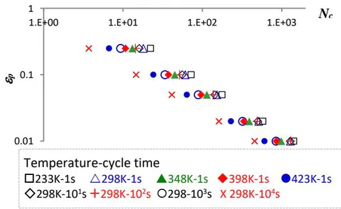Illustration and Validation The experimental creep fatigue data of Sn37Pb under cyclic triangular stress-time stressing generated by Shi et al. [26] has been analysed and the fitting constants, $C_b$ and $\beta_{b}$, for nine sets of $(\varepsilon_p,N_{cf})$ data have been extracted and these are tabulated in Table 1 [23]. Using these fitting constants, the $(\varepsilon_p,N_{cf})$ data were regenerated and these are depicted in Figure 6. Table 1: Sn37Pb: Extracted Creep Fatigue Fitting Constants [23] <table><tr><td rowspan="2">Creep-fatigue coefficients</td><td colspan="5">Temperature (K) at tc=1 sec</td></tr><tr><td>233K</td><td>298K</td><td>348K</td><td>398K</td><td>423K</td></tr><tr><td>Cb</td><td>2.76</td><td>2.22</td><td>1.70</td><td>1.43</td><td>0.97</td></tr><tr><td>βb</td><td>0.775</td><td>0.755</td><td>0.745</td><td>0.75</td><td>0.715</td></tr><tr><td rowspan="2">Creep-fatigue coefficients</td><td colspan="5">Cycle time, tc(s) at T=298 K</td></tr><tr><td>10^0 s</td><td>10^1 s</td><td>10^2 s</td><td>10^3 s</td><td>10^4 s</td></tr><tr><td>Cb</td><td>2.22</td><td>1.92</td><td>1.67</td><td>1.23</td><td>0.60</td></tr><tr><td>βb</td><td>0.755</td><td>0.735</td><td>0.715</td><td>0.715</td><td>0.670</td></tr></table>  Figure 6: Sn37Pb: Regenerated Experimental Creep Fatigue Data It is clear from Eq. (20) that a set of creep fatigue data, $(\varepsilon_{p},N_{cf})$, can be transformed into a set of pure fatigue data, $(\varepsilon_{p,ref},N_{f})$, by transforming the magnitude of $\varepsilon_{p}$ into $\varepsilon_{p,ref}$ using the relation, $$ \varepsilon_ {p, r e f} = \frac {\varepsilon_ {p}}{c \left(\varepsilon_ {p} , T , t _ {c}\right)}. \tag {31} $$ Let $c\big(\varepsilon_p,T,t_c\big) = 1 - X_k\big(\varepsilon_p\big)\eta_k(T,t_c)$, where $X_{k}\big(\varepsilon_{p}\big) = a_{k}\varepsilon_{p}^{b_{k}}$, the optimum values of $C_o,\beta_o,a_k,b_k$, and $H / k,B_{c},t_{c\infty}$ corresponding to the three cyclic parameter functions have been established through regressing the transformed fatigue data $(\varepsilon_{p,ref},N_f)$ with the pure fatigue equation, $\varepsilon_{p,ref} = C_{o}N_{f}^{-\beta_{o}}$. The optimum values are tabulated in Table 2 completes with the relative magnitude of regression difference. The collapsed data of $(\varepsilon_{p,ref},N_f)$ corresponding to the three cyclic parameter functions are depicted in Figure 7. Table 2: Sn37Pb: Fitting Constants for Creep Integrated Fatigue Equation Based on the Rate Equations of Sherby-Dorn, Larson-Miller, and Manson-Haferd <table><tr><td rowspan="2">Rate equations</td><td colspan="2">Fatigue coefficients</td><td colspan="2">x=aεpb</td><td rowspan="2">Fitting constant for η(T,tc)</td><td rowspan="2">Relative magnitude of regression residue</td></tr><tr><td>Co</td><td>βo</td><td>a</td><td>b</td></tr><tr><td>Sherby-Dorn</td><td>1.85</td><td>0.740</td><td>8.40x108</td><td>6.93x10-2</td><td>H/k= 8.98x103</td><td>3.4</td></tr><tr><td>Larson-Miller</td><td>6.58</td><td>0.806</td><td>1.17x10-4</td><td>4.43x10-2</td><td>Bc= 4.39x107</td><td>2.8</td></tr><tr><td>Manson-Haferd</td><td>3.75</td><td>0.773</td><td>-2.00x10-2</td><td>5.00x10-2</td><td>tcc∞= 2.34x107</td><td>1</td></tr></table>    Figure 7: Sn37Pb: Transformed Pure Fatigue Data using the Rate Equations of (a) Sherby-Dorn, (b) Larson-Miller and (c) Manson-Haferd 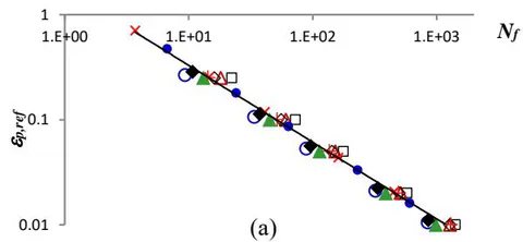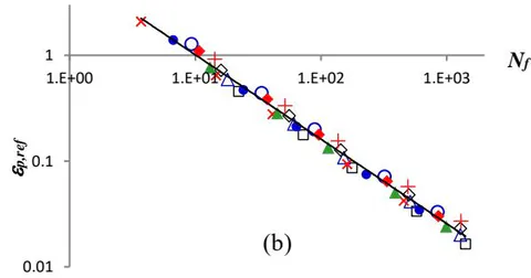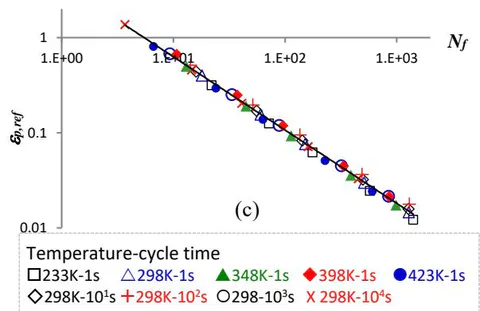It is noted that the fractional fatigue capability function that is based on the Manson-Hafred parameter returns a much smaller magnitude of regression residue than the other two parameter functions. This is consistent with the reported superior description of creep rupture of metal alloys for the Manson-Hafred parameter over the other two parameters [17]. Indeed, the magnitude of the fatigue capacity, $C_{o}$, given by the Sherby-Dorn parameter function was impossibly low – lower than the magnitude of $C_{b}$ – while that given by the Larson-Miller parameter function appears to be unrealistically high. ## IV. DISCUSSIONS The creep integrated fatigue equation integrates seamlessly the damages of creep and fatigue over the range from pure creep to pure fatigue. Comparing to the approach of the damage summation method, the creep integrated equation offers a more cohesive account for the combined damages of creep and fatigue. It does away with the challenging characterisation experiment that is required for the strain range partitioning method. More valuably, the method can be generalised to model metal fatigue that is aggravated by a generalised damage driving force, $X$, whose rate of growth of damage may be expressed in the form $$ \dot {x} = g (\mu) h (T, t), \tag {32} $$ where $g(\mu)$ is a function of the magnitude of the damage driving parameter (for example, $\mu \to \sigma$ in the case of creep being the damage driving force) while $h(T, t)$ is a function of temperature and time. The rate function, Eq. (32), shall then be expressed into the form: $$ \hat {g} (\mu) \hat {h} (T, t) = 1 \tag {33} $$ such as that shown in Eq. (23). The function $\hat{g} (\mu)\hat{h} (T,t)$ is the damage function for the damage driving force $X$. The damage force integrated fatigue equation is then given by $$ \varepsilon_ {p} = C _ {o} c (\mu , T, t _ {c}) N _ {x f} ^ {- \beta_ {o}}, \tag {34} $$ wherein $$ c (\mu , T, t _ {c}) = 1 - \widehat {g} (\mu) \widehat {h} (T, t _ {c}). \tag {35} $$ The magnitude of $c(\mu, T, t_c)$ ranges from nil to unity corresponding to the case of pure fatigue and pure $X$ damage, respectively. Let the damage function, $\hat{g}(\mu)$, takes the form $\hat{g}(\mu) = a\mu^b$, the fitting constants, $C_o, \beta_o, a, b$, and that associated with $\hat{h}(T, t_c)$ may be extracted through regression as illustrated in the previous section. In case of a metal fatigue that is aggravated by $n$ damage driving forces, Eq. (34) may be further generalised to integrate these damage forces, $X_{1},X_{2}\ldots X_{n}$, into the fatigue equation: $$ \varepsilon_ {p} = C _ {o} c _ {1} \left(\mu_ {1}, T, t _ {c}\right) c _ {2} \left(\mu_ {2}, T, t _ {c}\right) \dots c _ {n} \left(\mu_ {n}, T, t _ {c}\right) N _ {x f} ^ {- \beta_ {o}}, \tag {36} $$ where $c_{j}(\mu_{j},T,t_{c}) = 1 - \hat{g}_{j}\bigl (\mu_{j}\bigr)\hat{h}_{j}(T,t_{c}),\quad j = 1,2,\ldots n,$ (37) and $\hat{g}_j(\mu_j)$ may be conveniently assumed to be a power law relation, $a_{j}\mu_{j}^{b_{j}}$. In the absence of interaction between the damage forces, the coefficients, $a_{j}$ and $b_{j}$, of individual damaging force may be established individually by holding off other damaging forces. It is worth mentioning that the Basquin equation, $\sigma = C_{\sigma}N_{f}^{-\beta_{\sigma}}$, may be substituted for the Coffin-Manson equation in Eq. (34) in the case of an environmentally aggravated high cycle fatigue situation. ## V. CONCLUSIONS Creep fatigue analysis of solder joints in electronic assemblies has been presented. The condensed presentation comprised two major analyses: thermomechanical analysis and creep fatigue life modelling. The advanced analytical analysis can optimize the geometry of solder joints to minimise the magnitude of stresses in solder joints. This has led to the ideal geometry of stout hourglass for solder joints. The creep integrated fatigue equation integrates cohesively the damages of creep and fatigue over the range from pure creep to pure fatigue. The methodology can be generalised to model metal fatigue that is aggravated by multiple damaging forces.

Generating HTML Viewer...