## I. INTRODUCTION Telecommunication companies find it more economical advantageous in maintaining and keeping existing customers rather than loose them and bringing in new ones. The majority of telecom firms view their customers as their most valuable asset. For many markets, maintaining good customer relations is an important yet costly endeavor. This is especially crucial for the telecom industry, as companies that have made significant infrastructure investments. Existing customers are invaluable assets due to their established relationship with the company, which translates into ongoing revenue and lower marketing costs. Moreover, retaining customers can enhance brand loyalty, improve customer lifetime value, and boost overall profitability (Kumar & Shah, 2004). Conversely, losing existing customers can have substantial disadvantages. High churn rates can lead to significant revenue losses, increased acquisition costs for new customers, and a potential decline in market share. Additionally, customer attrition can negatively impact brand reputation and disrupt the stability of the customer base (Reinartz & Kumar, 2002). To mitigate these risks, telecom companies have historically employed various approaches to predict customer attrition. Early methods included statistical techniques such as logistic regression and decision trees, which provided valuable insights but often struggled with complex, non-linear relationships within the data (Berry & Linoff, 2004). More recently, advancements in machine learning have introduced sophisticated techniques like support vector machines (SVMs) and ensemble methods, which offer improved accuracy and predictive power (Friedman 2001). In order to forecast customer attrition, deep neural networks (DNNs) have become extremely effective tools in this field. DNNs can process big and complicated information. Using their capacity to recognize complex links and patterns, DNNs can offer telecom businesses insightful information that lowers churn rates (Adwan et al., 2014; Vural et al., 2020). The use of feature engineering in DNNs for churn prediction is crucial. Relevant features that telecom companies can extract include conversation duration, data consumption, billing history, and consumer demographics. These features are then fed into a neural network. Studies conducted by Vural et al. (2020) emphasize how crucial feature selection and preprocessing are to raising the predicted accuracy of the model. Feature sets that are well-designed improve the DNN's capacity to identify faint signals that point to possible churn. When it comes to capturing temporal dependencies in client behavior, DNNs are especially useful. They are able to determine consumption trends and changes over time by analyzing a customer's historical data. The scalability of DNNs is another important benefit. With DNNs, telecom businesses can effectively manage this big data dilemma as they gather enormous amounts of client data. Employing designs such as convolutional neural networks (CNNs), deep feed forward neural networks, or more sophisticated models like deep auto encoders, businesses are able to sort through massive information and identify minute customer behaviors that point to churn risk. Researchers using deep learning frameworks and distributed computing platforms, such (Almufadi et al. 2019) have demonstrated the scalability of DNNs for telecom churn prediction. For telecom companies, churn prediction with deep neural networks (DNNs) presents a promising way to keep customers. DNNs are a valuable tool for customer churn prediction because they can automatically learn complex patterns, handle temporal dependencies, and scale to large datasets. By optimizing feature engineering and utilizing sophisticated architectures such as CNNs and RNNs, telecom companies can leverage the predictive power of deep learning to improve customer retention and lower churn rates. A major problem in the telecom sector is customer attrition, or the loss of subscribers. Telecom providers must correctly identify the consumers at risk of leaving in order to solve this issue. While traditional churn prediction models have provided valuable insights, there is an increasing demand for more accurate, data-driven solutions. Deep Neural Networks (DNNs) offer a promising approach due to their ability to handle large volumes of heterogeneous customer data and identify complex patterns that traditional methods might overlook. However, the application of DNNs to churn prediction in telecom is not without challenges. To effectively harness DNNs, telecom companies must design, train, and deploy models capable of efficiently processing massive, diverse, and time-dependent customer data while maintaining interpretability and scalability. Addressing these challenges is crucial for developing accurate and actionable churn prediction systems that can significantly reduce customer churn and enhance customer retention strategies. ## II. REVIEW OF RELATED WORKS Baby et al. (2023) examined customer churn prediction in the banking sector using Artificial Neural Networks (ANNs). The methodology involved training the ANN model with input features to predict churn as the independent variable. The model was developed by adjusting hyper parameters, utilizing the forward propagation algorithm, and applying cross-validation techniques. Forward propagation involves passing input data through the network layers, calculating outputs, and updating model parameters accordingly. Hyper parameter tuning included optimizing aspects like learning rate, hidden layers, and neuron counts, while cross-validation ensured the model's robustness and ability to generalize. The ANN model achieved an accuracy of $86\%$ in predicting churn, outperforming a logistic regression model and demonstrating its effectiveness in capturing complex data relationships. This high accuracy underscores the ANN model's superior performance in identifying potential churners. The study highlights the practical value of this model for the banking industry, where it can be used to proactively identify at-risk customers and implement effective retention strategies. Sikri et al. (2024) tackled customer churn prediction using machine learning, addressing challenges related to imbalanced and diverse data distributions in churn datasets. The study introduced a novel Ratio-based data balancing technique during preprocessing to mitigate data skewness, a common issue leading to biased models. The research evaluated several algorithms, including Perceptron, Multi-Layer Perceptron, Naive Bayes, Logistic Regression, K-Nearest Neighbour, Decision Tree, and ensemble methods like Gradient Boosting and XGBoost. These algorithms were tested on datasets balanced using the proposed technique and traditional resampling methods like Over-Sampling and Under-Sampling. Results showed that the Ratio-based technique significantly outperformed traditional methods, enhancing churn prediction accuracy. Ensemble algorithms, particularly Gradient Boosting and XGBoost, delivered superior results compared to standalone methods, with the best outcomes achieved using a 75:25 data ratio and XGBoost. The study highlighted the effectiveness of this approach in improving model performance, as measured by Accuracy, Precision, Recall, and F-Score. Oladipo et al. (2023) focuses on predicting customer churn in the telecommunications industry using an ensemble-based approach. The model integrates several machine learning algorithms, including XG Boost, Light GBM, Random Forest (RF), and Cat Boost. These algorithms are combined using a stacking technique, which involves training multiple models and then combining their predictions to improve overall performance. Metaheuristics are also developed to enhance the predictive capabilities of the ensemble model. The model leverages ensemble learning, a technique that improves prediction accuracy by combining the strengths of various machine learning algorithms. Stacking is used to integrate XG Boost, Light GBM, RF, and Cat Boost, each contributing unique strengths to the predictive model. This approach helps the telecommunications company predict customer attrition by analyzing patterns in customer data and identifying those most likely to churn. The use of metaheuristics further refines the model, optimizing its performance. The result showed that the ensemble-based model achieved an impressive accuracy of $92.2\%$ in predicting customer churn. This high level of accuracy demonstrates the effectiveness of combining multiple algorithms through stacking and metaheuristics in forecasting customer attrition. The results highlight the model's capability to accurately identify at-risk customers, providing valuable insights for the telecommunications industry to enhance customer retention strategies. Suh, Y (2023) presented the application of a machine learning algorithm to predict customer churn in the rental business sector, specifically for a water purifier rental company. The algorithm was trained on a large dataset to learn meaningful features that contribute to churn. Performance metrics such as the F-measure and Area Under Curve (AUC) were used to evaluate the model's effectiveness. The model was developed by analyzing customer behavior data from a Korean electronics company's rental service. The dataset used for training and testing contained approximately 84,000 customers, providing a substantial basis for the algorithm to learn from. The model's performance was further validated using a larger dataset of about 250,000 customers to test its predictive capabilities in real-world scenarios. The model not only predicted churn but also identified key variables influencing churn, which could be used by customer management staff to implement targeted marketing strategies. The model achieved impressive results, with an F1 score of $93\%$ and an AUC of $88\%$, indicating strong predictive accuracy and reliability. Additionally, the model's inference performance on a larger operational dataset demonstrated a hit rate of about $80\%$, confirming its effectiveness in predicting actual churn cases. The identification of influential variables on churn provided actionable insights for personalized marketing efforts, helping the company address churn causes more effectively. Dhangar & Anand (2021) reported a comprehensive methodology for predicting customer churn across various industries. The approach begins with data pre-processing and exploratory data analysis, followed by feature selection. The dataset is then split into training $(80\%)$ and testing $(20\%)$ sets. Multiple machine learning algorithms, including Logistic Regression, Naive Bayes, Support Vector Machine (SVM), and Random Forest, are applied to the training data. Ensemble techniques are also utilized to assess their impact on model accuracy. K-fold cross-validation is employed for hyperparameter tuning and to prevent overfitting. Finally, the models' performance is evaluated using the AUC/ROC curve. The results indicate that Random Forest achieved the highest accuracy $(87\%)$ and the best AUC score $(94.5\%)$, making it the most effective model for predicting customer churn in this study. The SVM classifier also performed well, with an accuracy of $84\%$ and an AUC score of $92.1\%$. These results suggest that Random Forest, followed closely by SVM, outperforms other models in predicting customer churn. Abou-el-Kassem et al. (2020) presented a dual-approach methodology to address customer churn in the telecom sector. The first approach involves identifying key factors influencing customer churn using machine learning algorithms such as Deep Learning, Logistic Regression, and Naive Bayes. A dataset is built from practical questionnaires to facilitate this analysis. The second approach focuses on predicting customer churn by analyzing user-generated content (UGC) from social media platforms. Sentiment analysis is applied to this UGC to determine text polarity, categorizing it as positive or negative. The results indicate that the machine learning algorithms employed-Deep Learning, Logistic Regression, and Naive Bayes-achieved similar accuracy levels in predicting customer churn. However, the algorithms differed in how they weighted the importance of various attributes in the decision-making process. This suggests that while the models are equally effective in accuracy, they prioritize different factors when making predictions. Hamuntenya & Iyawa (2023) reported the application of four machine learning algorithms (K-Nearest Neighbors, Random Forest, Gradient Boosting Tree, and XGBoost) to predict customer churn for MTC Namibia, a mobile network operator. The use of these algorithms reflects a common approach in churn prediction, where machine learning techniques are employed to analyze customer behavior and predict potential attrition. The model focused on key factors such as real monthly usage, plan choice, and payment methods. These features were used as inputs to train the models. The performance of the models was evaluated using the ROC-AUC (Receiver Operating Characteristic - Area Under the Curve) score, a metric that measures the model's ability to distinguish between classes (churn and no churn). Among the algorithms tested, XGBoost emerged as the top-performing model, achieving an accuracy rating of $84\%$ based on the ROC-AUC score. The study also identified that specific factors-real monthly usage, plan choice, and payment method-significantly influence churn rates, highlighting the importance of these variables in predicting customer attrition. Zhao (2023) focused on predicting customer churn in a banking context using two machine learning algorithms: Random Forest and Decision Tree classifiers. The methodology begins with data preprocessing, which involves cleaning and adjusting the dataset by removing irrelevant features and renaming feature names for better accessibility during analysis. The dataset is then split into training and testing sets using an 80-20 split. The study proceeds by building churn prediction models with the selected algorithms. Feature selection is performed to identify the most significant variables, and their importance is visualized using bar graphs. Both models are trained on the training set and subsequently tested on the testing set. The performance of the models is evaluated using confusion matrices and accuracy scores, which are standard tools for assessing classification models. The visualization of these metrics allows for a clear comparison of model effectiveness. The results indicate that both the Random Forest and Decision Tree models successfully predict customer churn, with the Random Forest model outperforming the Decision Tree model. The Random Forest model achieved a higher accuracy score of $91\%$, making it the more effective algorithm in this study. Calis & Kozlowska (2021) focused on predicting customer churn using various data mining techniques and classification algorithms within a machine learning framework. The methodology involves analyzing a dataset of 7,166 customer records from a telecommunications company. The study aims to identify the most effective algorithms: logistic regression, K-Nearest neighbor, Decision tree, random forest, Support Vector Classifier for accurately predicting customer churn. The process begins with data preprocessing, which includes scaling and applying log transformations to the data, likely to normalize the features and enhance model performance. Classification algorithms are employed to build predictive models, although the abstract does not specify which algorithms were used. The results show that logistic regression was the top performing model with an accuracy of $81\%$ and also had the best recall and decision tree was closely following with an accuracy of $57\%$. Their work indicated that the model struggled with an unbalanced data which affected the performance of the models. According to other metrics, the best model is the decision tree because it produced a better recall outcome. Shrestha & Shakya (2019) addressed a critical issue in the telecommunications industry: customer churn, which significantly impacts revenue. The study emphasizes the importance of effective churn management for gaining a competitive edge by improving customer retention rates. The research highlights the challenge of handling imbalanced datasets in churn prediction, particularly with real-world telecommunication data that may differ from publicly available datasets. The methodology involves applying the XGBoost machine learning algorithm to both a native dataset from a major telecommunications company in Nepal and a publicly available dataset. The native dataset comprises 52,332 customer records, with a significant imbalance between non-churned (46,204) and churned (6,128) customers. The performance of XGBoost on this dataset is impressive, yielding an accuracy of $97\%$ and an F1-score of $88\%$. Additionally, the study compares results with a publicly available dataset of 3,333 subscribers, achieving slightly lower but still strong accuracy $(96.25\%)$ and F1-score $(86.34\%)$. The high accuracy and F1-scores underscore the algorithm's effectiveness in predicting customer churn, offering valuable insights for telecom companies aiming to improve retention strategies. ## III. METHODOLOGY The proposed customer attrition model in a telecom company is a machine learning approach to solving churn problems. It involves the evaluation of the performance and effectiveness of DNN model in customer attrition. The implementation of a Deep Neural Network (DNN) for forecasting customer attrition involves a systematic approach to building a robust predictive model capable of accurately identifying customers at risk of churn. The process begins with the acquisition and preprocessing of telecom customer data, including handling missing values, and normalizing features. Feature engineering and selection are then performed to identify the most relevant attributes that influence customer attrition. The DNN model is constructed with multiple layers to capture complex patterns within the data. Hyperparameters, including learning rate, batch size, and the number of hidden layers, are fine-tuned through methods such as cross-validation to optimize the model's performance. The trained model is then evaluated using metrics like accuracy, precision, recall, and F1-Score, demonstrating its effectiveness compared to traditional machine learning methods. The successful deployment of this DNN model enables the telecom firm to proactively identify and retain at-risk customers, thereby improving customer satisfaction and reducing churn-related revenue losses. The system's architectural framework shown in figure 1 involves the design and organization of the components, layers and processes that is involved in the prediction system. It guides the development and implementation of the system and ensures that the system is efficient, scalable and capable of providing actionable insights for customer retention.  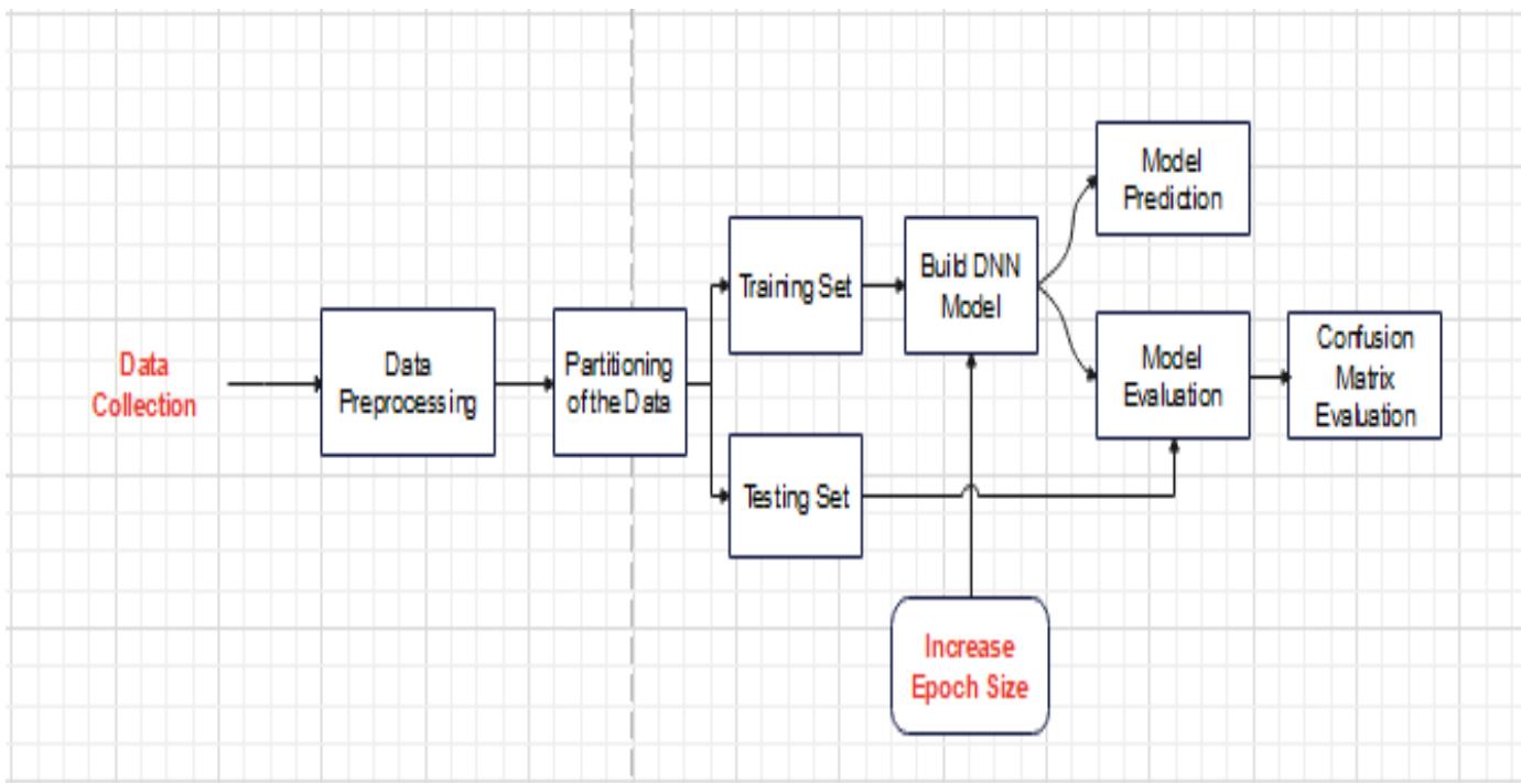Figure 1: Architectural Framework of the Customer attrition for a Telecom Company ## IV. MODEL DEVELOPMENT ### a) DNN Model Development In developing the DNN model, we selected a DNN architecture that is suited for the challenge according on its complexity. The deep feed forward networks with several hidden layers was adopted. The model's input features were Specified, these are the churn-related features and pertinent customer data that were prepared during the data pretreatment stage. To ascertain the total number of neurons in each layer as well as the number of hidden layers, several architectures were examined to determine the one that works best for the dataset, the right activation functions was selected for the hidden layer neurons, which is the Sigmoid functions which mapped input to value between 0 and 1 which is suitable for binary classification problems, $\sigma(x) = 11 + e - x \backslash \text{sigma}(x) = \backslash \text{frac}\{1\} \{1 + e^{\wedge} \{-x\}$ $\sigma(x) = 1 + e - x1$ and ReLUs (Rectified Linear Units) $\text{ReLU}(x) = \max(0, x)$ was also selected, as it mapped all negative values to 0. An output layer was created that generates a customer attrition. The developed deep neural network architecture is shown in Figure 2.  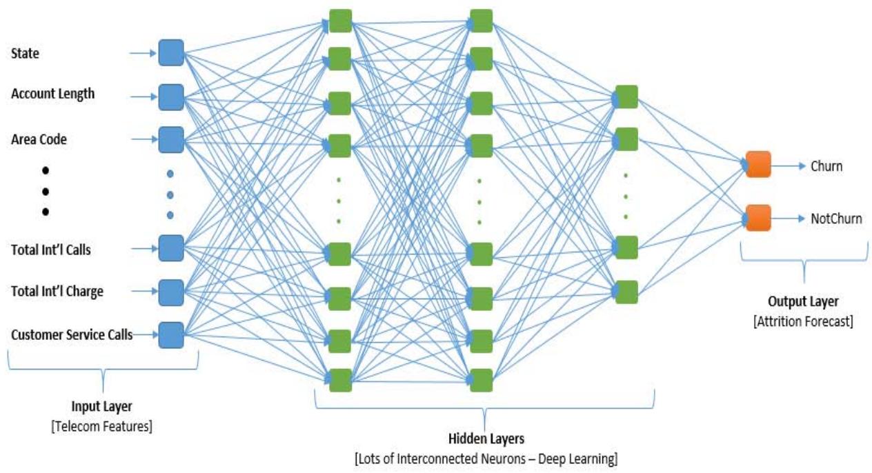Figure 2: Developed Deep Neural Network Architecture Loading of Dataset Code Snippet The dataset is loaded as input into the DNN architecture. The already downloaded file is stored in a folder in the system where the code file is stored and is easily loaded to the system for manipulation by the model. ### b) Code Snippets for Model Development The code snippet shown above is the developed DNN model/ architecture used for the training of the dataset to learn the patterns in the dataset to be able to forecast attrition with new unseen data. The model uses the ReLu activation function in the hidden layers and the sigmoid activation function in the output layer of the model. ### c) Model Training The size of the dataset is 3,333 instances and $80\%$ was used to train the model while $20\%$ was used for testing. We Selected a loss function that measures the discrepancy between the actual churn labels and the model's predictions, the binary cross-entropy technique was used. The Binary Cross-Entropy also called Log Loss is the standard loss function for binary classification problems and It is suitable for this task, as it works well with models that output probabilities, it also measures how far the predicted probabilities are from the actual binary labels (0 or 1). ### d) Model Optimization To enhance the model's performance and ensure its ability to generalize well to unseen data, a combination of advanced model optimization techniques, including hyper-parameter tuning, regularization, and early stopping where chosen. Each of these methods played a critical role in improving the accuracy, stability, and generalization ability of the model. ### e) Hyper-parameter Tuning Essential hyper-parameters such as the number of neurons in each layer were optimized, the number of hidden layers, batch size, and learning rate. To systematically and efficiently search for the optimal set of hyper-parameters, Bayesian optimization was adopted. This technique constructs a probabilistic model of the objective function and uses it to select the most promising hyper-parameters to evaluate next. Compared to grid or random search, Bayesian optimization reduces the number of trials required to reach near-optimal performance. To address the issue of overfitting and enhance the model's generalization capability, we applied regularization techniques, namely:L1 Regularization (Lasso), by Introducing a penalty equal to the absolute value of the magnitude of coefficients, encouraging sparsity in the model; L2 Regularization (Ridge) by Adding a penalty proportional to the square of the magnitude of coefficients, discouraging large weight values; and Dropout Layers, where a random subset of neurons is deactivated in each training iteration, thereby reducing reliance on specific features and improving robustness. These regularization strategies helped control model complexity and prevent it from memorizing the training data. When validation loss began to increase, indicating that the model was starting to over fit the training data, these regularization techniques ensured that the final model retained strong predictive power without unnecessary training iterations ### f) Feature Scaling The application of feature scaling to the dataset helped to prevent feature dominance, where features with large ranges dominate the model. The steps adopted to apply feature Scaling are 1. Importation of necessary libraries: from sklearn.preprocessing import StandardScaler 2. Creation of a scalar object: scalar = StandardScaler() 3. Fit theScaler object to the data:Scaler.fit(X train) 4. Transformed the data: X_trainScaled = scalar.transform(X_train) 5. Applied the same scaling to the test data: X_testScaled =Scaler.transform(X_test) For Feature Selection which helped reduce dimensionality, improve model performance, and prevent over fitting. Steps followed; 1. Importation of necessary libraries: from sklearn. feature_selection import Select K Best, mutual_info_classif 2. Created a feature selector object: selector = Select K Best (mutual_info_classif, k=10) `k` determines the number of features to select. 3. Fitted the selector to your data: selector.fit(X_train, y_train) this step calculates the mutual information between each feature and the target variable. 4. Transform your data: X_train_selected = selector.transform(X_train) this step applies the feature selection to your training data. 5. We applied the same selection to the test data: X_test_selected = selector.transform(X_test) this ensures that the same features are selected for both training and testing. ### For Handling imbalanced datasets The SMOTE (Synthetic Minority Over-Sampling Technique) Techniques helped address class imbalance issues in attrition datasets. importation of libraries: from imblearn.over_sampleing import SMOTE 1. Creation of a SMOTE object: smote = SMOTE(random_state=42) random_state ensures reproducibility of the results. 2. Fitted the SMOTE object to the data: X_train_resampled, y_train_resampled = smote.fit_resample(X_train, y_train) These step generated synthetic samples of the minority class and were combined with the original data. These formulas provide a mathematical foundation for understanding how Feature Scaling, Feature Selection, and SMOTE work. $$ Standardization (Z-Score Normalization): `z = (x - μ) / σ` $$ - `x': original feature value - `\mu`: mean of the feature - `o`: standard deviation of the feature - `z`: scaled feature value $$ Min-Max Scaling: `xScaled = (x - x_min) / (x_max - x_min)` $$ - `x': original feature value - `x min': minimum value of the feature - `x_max': maximum value of the feature - `xScaled`: scaled feature value #### Feature Selection Mutual Information: $\mathrm{I}(\mathrm{X};\mathrm{Y}) = \sum_{\mathrm{p}}\mathrm{p}(\mathrm{x},\mathrm{y})$ $\log (\mathsf{p}(\mathsf{x},\mathsf{y}) / (\mathsf{p}(\mathsf{x})\mathsf{p}(\mathsf{y})))$ `X`: feature Y\*:target variable - `p(x,y) `: joint probability distribution of `X` and `Y` - `p(x)': marginal probability distribution of `X' - `p(y)': marginal probability distribution of `Y' `I(X;Y)': mutual information between `X' and `Y' SMOTE $$ Synthetic Sample generation `x_synthetic = x_i + (x_zi - x_i) * \delta` $$ `x_i`: minority class sample - `x zi`: another minority class sample (randomly selected) - `\delta`: random number between 0 and 1 - `x_synthetic': synthetic sample generated ## V. RESULTS The exploratory data analysis (EDA) is used to understand the distribution of data and variable relationships. From the results obtained, key patterns and features associated with customer attrition that facilitate informed decision-making process for the telecom firm are shown in table 1. The model validation graphs for 10 and 100 epochs are presented in figure 3 and figure 4 respectively, while table 2 and table 3 shows their respective confusion matrices. The statistical result summary is presented in table 4. <table><tr><td>Features</td><td>Mean Decrease Gini</td></tr><tr><td>State</td><td>98.903401</td></tr><tr><td>Account Length</td><td>17.928327</td></tr><tr><td>Area Code</td><td>4.709509</td></tr><tr><td>International Plan</td><td>52.726265</td></tr><tr><td>Voice Mail Plan</td><td>8.992156</td></tr><tr><td>Number of Vmail Messages</td><td>14.876575</td></tr><tr><td>Total Day Minutes</td><td>76.118072</td></tr><tr><td>Total Day Calls</td><td>17.505372</td></tr><tr><td>Total Day Charge</td><td>78.532000</td></tr><tr><td>Total Eve Minutes</td><td>33.655187</td></tr><tr><td>Total Eve Calls</td><td>15.715358</td></tr><tr><td>Total Eve Charge</td><td>34.138874</td></tr><tr><td>Total Night Minutes</td><td>20.181908</td></tr><tr><td>Total Night Calls</td><td>17.074633</td></tr><tr><td>Total Night Charge</td><td>19.820026</td></tr><tr><td>Total Intl Minutes</td><td>25.868424</td></tr><tr><td>Total Intl Calls</td><td>29.046591</td></tr><tr><td>Total Intl Charge</td><td>24.009036</td></tr><tr><td>Customer Service Calls</td><td>73.435423</td></tr></table>   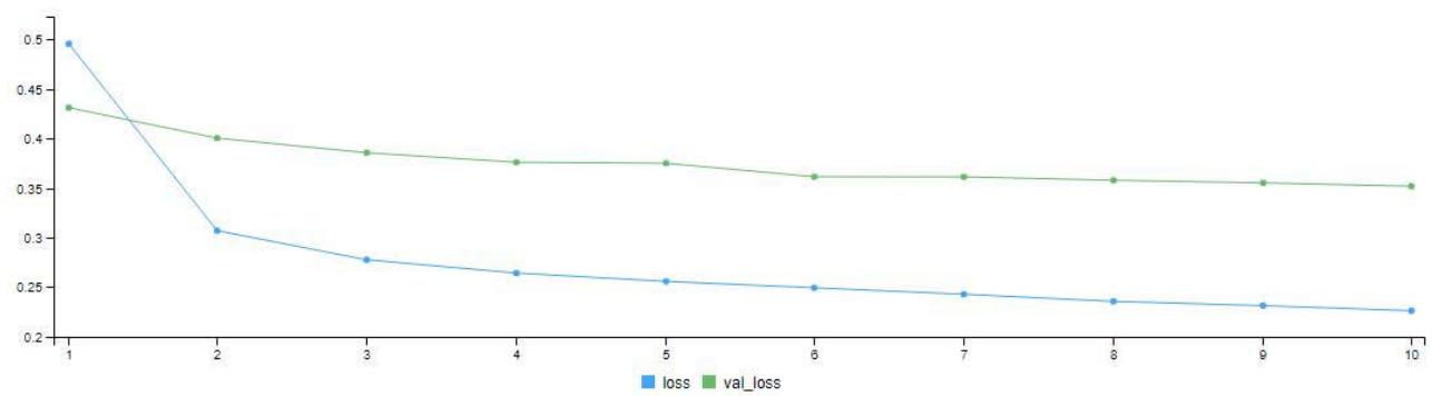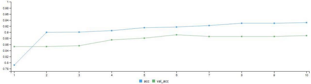Figure 3: Model Validation Graph for 10 Epoch (Iteration)   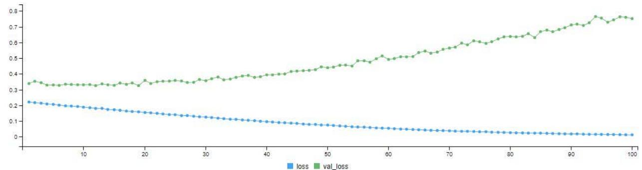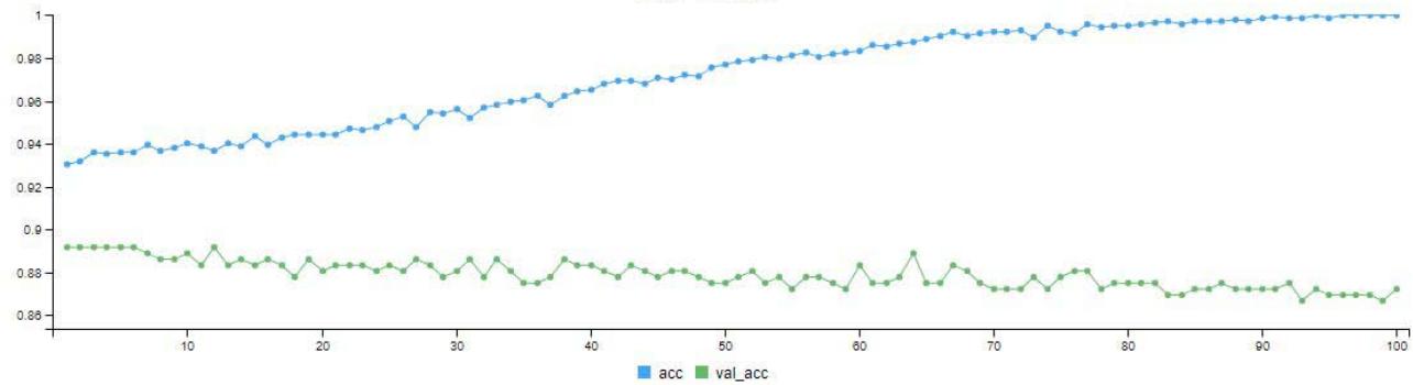Figure 4: Model Validation Graph for 100 Epoch (Iteration) <table><tr><td rowspan="2">Prediction</td><td colspan="2">Reference</td></tr><tr><td>0</td><td>1</td></tr><tr><td>0</td><td>397</td><td>36</td></tr><tr><td>1</td><td>3</td><td>13</td></tr></table> <table><tr><td rowspan="2">Prediction</td><td colspan="2">Reference</td></tr><tr><td>0</td><td>1</td></tr><tr><td>0</td><td>389</td><td>29</td></tr><tr><td>1</td><td>11</td><td>20</td></tr></table> <table><tr><td></td><td>Precision</td><td>Sensitivity</td><td>Specificity</td><td>P-Value</td><td>Accuracy</td></tr><tr><td>10 Epoch</td><td>92%</td><td>99%</td><td>27%</td><td>2.99e-07</td><td>91%</td></tr><tr><td>100 Epoch</td><td>93.1%</td><td>97%</td><td>41%</td><td>0.00719</td><td>98.1%</td></tr></table> ## VI. DISCUSSION OF RESULTS The model training was done twice with 10 and 100 epochs (i.e. iterations). Figure 3 is the model validation graph for 10 iterations. It shows the loss - validation loss and accuracy - validation accuracy of the model. We can see the loss line (blue line) coming far below the validation loss line (green line). At the final iteration, the loss line came down to a little above 0.2 mark. The accuracy of the model also climbed from $78\%$ to a little above $90\%$ as seen in the graph. In Figure 4.6, after the 100 iterations, we can see the loss line (blue line) coming far below the validation loss line (green line). At the final iteration, the loss line came down below 0.1 mark. The accuracy (blue line) of the model also climbed from $93\%$ to above $98\%$ as seen in the graph. In Figure 4. after the 100 iterations, we can see the loss line (blue line) coming far below the validation loss line (green line). At the final iteration, the loss line came down below 0.1 mark. The accuracy (blue line) of the model also climbed from $93\%$ to above $98\%$ as seen in the graph. The misclassification table for 10 epoch as shown in Table 2 depicts that, from the reference (actual) prediction, 13 customers has churn intensions and the model predicted the same. The model also predicted that 397 customers has no plan of churning and the reference predicted the same. The model misclassified or was confused with 36 customers predicting that they have no plan of churning while the reference predicted otherwise and the model predicted that 3 customers has churn in mind while in actual case, it is otherwise. Table 3 is the misclassification table for 100 epochs. The model predicted 389 customers has no churn plans and the actual prediction was same. The model also predicted that, 20 customers will churn and the reference predicted same. However, the model was confused with some records in that, it predicted that 29 customers will not churn whereas in actual sense they churned as the model also misclassified 11 customers as it predicted that they will churn, but they didn't. Table 4 is the summary of the statistical results produced by the DNN model for customer attrition. From the table, we can see that there was a slight improvement when the model was trained with 100 epoch. The stochastic gradient descent (SGD) algorithm is employed for training and optimization, iteratively refining the model's parameters to enhance its predictive accuracy. Evaluation of the developed DNN model follows, utilizing common evaluation metrics such as accuracy, precision, recall, and the confusion matrix. Findings from the evaluation reveal promising results, with the model achieving a performance accuracy of $91\%$ after 10 epochs, and a slight improvement to $98.1\%$ after 100 epochs. Notably, there was a concurrent enhancement in precision, recording $92\%$ at 10 epochs and a further increase to $93.1\%$ after 100 epochs. There was reduction in sensitivity (recall), but generally, the model recorded an improvement when iterated 100 times. ## VII. CONCLUSION The study on customer attrition forecast for the telecom firm through the implementation of a Deep Neural Network (DNN) has provided valuable insights into the effectiveness of leveraging advanced machine learning techniques for customer retention strategies. Through the collection and integration of historical data from diverse sources, the preprocessing steps ensured the dataset's readiness for training a sophisticated DNN model. The careful splitting of the data into training and validation sets facilitated robust model development, allowing for iterative adjustments to enhance predictive accuracy. The implementation of the stochastic gradient descent (SGD) algorithm further optimized the DNN model, leading to commendable performance metrics. {"code_caption":[],"code_content":[{"type":"text","content":"7 # Load telecom churn dataset \n8 # Example dataset can be found here: https://www.kaggle.com/blastchar/telco-customer-churn \n9 telecom_data <- read.csv(\"churn-bigml-80.csv\") \n10 test_data <- read.csv(\"churn-bigml-20.csv\") "}],"code_language":"r"}

Generating HTML Viewer...

References

11 Cites in Article
O Adwan,H Faris,K Jaradat,O Harfoushi,N Ghatasheh (2014). Predicting customer churn in telecom industry using multilayer preceptron neural networks: Modeling and analysis.
Naseebah Almufadi,Ali Mustafa Qamar (2019). Deep Convolutional Neural Network Based Churn Prediction for Telecommunication Industry.
B Baby,Z Dawod,S Sharif,W Elmedany (2023). Customer churn prediction model using artificial neural network: A case study in banking.
M Barry,G Linoff (2004). Data Mining Techniques for Marketing, Sales and Customer Relationship Management.
Wiesław Matwiejczuk,Mariusz Gorustowicz (2021). Effectiveness determinants of investment and construction services.
Jerome Friedman (2001). Greedy function approximation: A gradient boosting machine..
L Hamuntenya,G Iyawa (2023). Enhancing customer retention: A study on churn prediction models for MTC Namibia using machine learning algorithms.
V Kumar,D Shah (2004). Building and sustaining profitable customer loyalty for the 21st century.
I Oladipo,J Awotunde,M Abdulraheem,F Taofeek-Ibrahim,O Obaje,J Ndunagu (2023). Customer churn prediction in telecommunications using ensemble technique.
E Abou El Kassem,S Ali,A Mostafa,F Alsheref (2020). Customer churn prediction model and identifying features to increase customer retention based on user-generated content.
K Dhangar,P Anand (2021). A review on customer churn prediction using machine learning approach.
No ethics committee approval was required for this article type.
Data Availability
Not applicable for this article.
How to Cite This Article
Emmah, Victor Thomas. 2026. \u201cDeep Neural Network Model for Customer Attrition Forecast in a Telecommunication Company\u201d. Global Journal of Computer Science and Technology - E: Network, Web & Security GJCST-E Volume 25 (GJCST Volume 25 Issue E1): .
Explore published articles in an immersive Augmented Reality environment. Our platform converts research papers into interactive 3D books, allowing readers to view and interact with content using AR and VR compatible devices.
Your published article is automatically converted into a realistic 3D book. Flip through pages and read research papers in a more engaging and interactive format.
The loss of customers is becoming a significant challenge for telecom companies due to the high cost of acquiring new customers and the critical need to retain existing ones. This dissertation explores the importance of predicting customer attrition in the telecommunications sector using a deep neural network (DNN) model. The study highlights the crucial role of customer retention in a highly competitive market. The system was developed using historical data, preprocessing techniques, and a customized DNN architecture. The methodology followed a DevOps approach, encompassing the collection, integration, and preprocessing of diverse datasets, followed by the construction and optimization of the DNN model with five layers using stochastic gradient descent. The findings demonstrate the model’s impressive accuracy, achieving 98.1% after 100 epochs, along with improved precision. The results underscore the DNN model’s effectiveness in predicting churn, emphasizing the value of iterative refinement through multiple training cycles.
Our website is actively being updated, and changes may occur frequently. Please clear your browser cache if needed. For feedback or error reporting, please email [email protected]
Thank you for connecting with us. We will respond to you shortly.