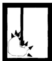
## I. INTRODUCTION Deformation modeling emerged as a direction in computer graphics, enabling the conversion of the kinematics of a physically observed object into a virtual reality. The concept of a deformable model is typically considered from the position of the mechanics of deformable solids. In accordance with this concept, the deformation process of a continuum can be conveniently described in Lagrangian coordinates. The paradigm of a deformable model is the "snake", the shape and geometry of whose "body" depend on the displacements of the key points [1, 2, 3]. Formally, a "snake" is a contour specified parametrically, usually as a cubic spline. The technology of approximating the initial contour with a spline is based on the procedure of minimizing a functional associated with the deformation energy of the contour, within the boundaries of the field surrounding each key point (fig. 1). 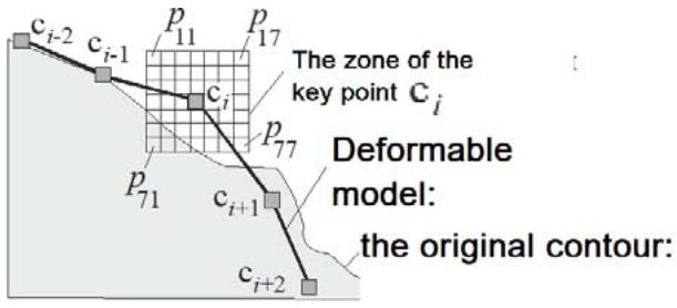 Fig. 1: Deformable "snake" model Approximation of the initial contour using a deformation model "snake" is widely used in biomedical research (computed tomography), as well as in artificial intelligence applications for motion tracking and object recognition. 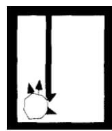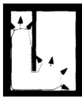Another approach to constructing a geometrically deformable model (GDM) is the concept based on the expansion of a virtual thin-walled balloon inside the boundaries of the scanned object (fig. 2). The mathematical apparatus used in GDM technology is the finite element method in the form of the displacement method. The balloon is modeled using finite elements in the form of thin-walled three-node plates. The geometry of the balloon at time $t$ is represented in parametric form [4, 5]. $$ R(u,v,t) = [\psi_x(u,v,t),\psi_y(u,v,t),\psi_z(u,v,t)] $$ Where $\psi_x, \psi_y, \psi_z$ - approximating cubic spline functions along the axes $x, y, z$; $u, v$ - dimensionless variables such that $u \in [0,1]$, $v \in [0,1]$. During the scanning of the internal cavity of the investigated object, each node of the finite element model is attracted to a point on the bounding contour in the normal direction (fig. 3). The current deformed state of the finite element is fully determined by the metric tensor [6, 7, 8]. $$ g(R(u,v,t)) = \frac{\partial R}{\partial u} \frac{\partial R}{\partial v} $$  Step 1  Step 2  Step 3 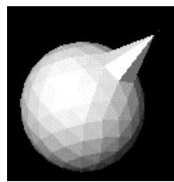 Fig. 2: Technology visualization GDM [6] According to [6], the adaptive algorithm is constructed such that at each step, the condition is satisfied at the nodes of the finite element mesh: $$ \alpha_ {0} D (x, y, z) + \alpha_ {1} I (x, y, z) + \alpha_ {2} T (x, y, z) \geq 0 \tag {1} $$ where $C(x,y,z)$ — the objective function associated with the current position of the node in the model; $D(x,y,z)$ — The deformation potential (a monotonically decreasing or increasing function); $I(x,y,z)$ — the constraint function, which "informs" the node of the finite element mesh that it may be in contact with a voxel (a raster element of the object); $T(x,y,z)$ — The topological information function, which prevents the nodes of the finite element model from penetrating the boundary of the object; $\alpha_0, \alpha_1, \alpha_2$ — weighting coefficients. Condition (1) causes the model to deform until all vertices reach the boundary of the scanned object. Another direction of deformation modeling is the analysis of the behavior of spatial truss structures, which experience large linear and angular displacements with small deformations during operation. In this case, the numerical solution of the geometrically nonlinear problem is based on the iterative Newton-Raphson procedure and the "correcting arc" method, the essence of which is the adaptive adjustment of the loading step size when approaching and after passing the bifurcation point [9, 10]. It should be noted that when calculating the rod system by the finite element method (FEM) taking into account large displacements, the tangent stiffness matrix is used. The construction of this matrix is based on the minimization of the deformation energy potential \[9\]: $$ \frac {\partial^ {2} U}{\partial y ^ {2}} + \frac {\partial U}{\partial y} = P ^ {(e)} $$ where $U$ - potential strain energy of a finite element (FE); $y$, $P^{(e)}$ — vectors of displacements and generalized external forces FE. As an illustration of the solution in the geometrically nonlinear formulation, let us consider a test example from [9, 11]. A flexible, curved beam with a rectangular cross-section of $1\mathrm{m} \times 1\mathrm{m}$, a radius of 100 m, and an arc angle of $45^{\circ}$, rigidly fixed at one end ( $x = 0$, $y = 0$, $z = 0$ ), is subjected to out-of-plane bending by a concentrated force $F = 100\mathrm{N}$. The coordinates of the free end of the beam in the initial position are [70.71; 70.71; 0] m. The mechanical constants of the beam material are: Young's modulus $E = 10\mathrm{MPa}$; Poisson's ratio $v = 0$. Figure 4 shows the results of the calculation performed using the nonlinear solver of the ANSYS software package [12]. The beam was discretized into 16 spatial beam-type finite elements BEAM4. 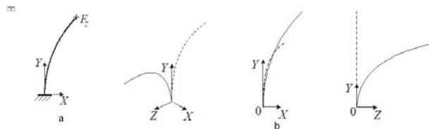 Fig. 4: Results of the analysis of the curved beam: a - initial state of the beam; b - visualization of the beam deformation relative to the initial position (dashed line) The coordinates of the displacement of the load application point were [46.84; 15.56; 53.66] m according to [9, 11] and [46.9; 15.6; 53.6] m in accordance with the ANSYS solution. As can be seen, the given displacement values are quite close. The above-presented concepts of deformation modeling are highly specialized and cannot be extended to problems in structural mechanics related to the study of kinematically transformable truss systems. In this regard, the development of a methodology for finite element modeling of rod structures, taking into account the structural shape change of the initial geometry, is an urgent task. ## II. MATERIALS AND METHODS We will conduct a study of a regular truss system, shown in its initial (undeformed) state in Fig. 5, considering the controlled displacement of the boundary nodes 1, 2,..., 6. In the separate fragments of Fig. 5, the letters L and B denote the grids formed by the hinge-rod (truss) and beam finite elements, respectively. In both cases, the nodal platforms S are modeled as practically non-deformable beam finite elements. The distinctive feature of this computational scheme compared to the scheme in [13] is the presence of the nodal platform S, modeled by rods with a modulus of elasticity exceeding the modulus of elasticity of the connecting rods by five orders of magnitude. From a structural point of view, the introduction of the platforms S allows us to conditionally account for the nodal connections of real truss systems. An example of the modeled structure of a real nodal connection is shown in Fig. 6 [14]. This node is a demountable structure with one central and six peripheral bolted connections, providing relative mobility of the truss members. 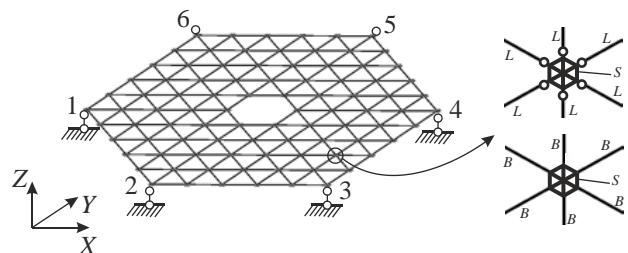 Fig. 5: The truss model in the initial (undeformed) state 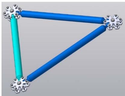 Fig. 6: The structure of the nodal connection [14] To investigate the process of shape, change of the truss structure, we will apply the modified Lagrangian method [15], the essence of which is in the discrete increment of the displacements of the boundary nodes and the reconstruction of the geometry of the finite element mesh in the current initial basis, taking into account the obtained nodal displacements. In the literature on structural mechanics, this type of nonlinearity is called genetic [16]. For the software implementation of this concept, we will use the APDL programming language [12], integrated into the ANSYS Mechanical software package. During the kinematic quasi-static shape change, internal forces will arise in the structural members due to the gravitational influence and structural connections. To assess the level of deformed state of the finite element model, we will use the values of the axial strain in the truss members. ## III. 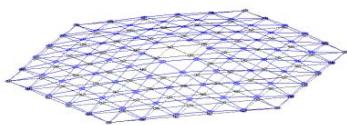RESEARCH RESULTS As an object of study, we consider a regular hexagonal truss system in plain view (Fig. 7). The lengths of the rods forming the regular lattice of the structure are $0.4\mathrm{m}$. The radius of the circumscribed circle of the platform S is $0.05\mathrm{m}$. The mechanical constants of the rods (aluminum alloy) are $\mathsf{E} = 70\mathrm{GPa}$, $\nu = 0.32$, density $\rho = 2885\mathrm{kg / m^3}$. The truss members and the S platforms have a tubular cross-section with an outer diameter of $18\mathrm{mm}$ and a wall thickness of $1.5\mathrm{mm}$. 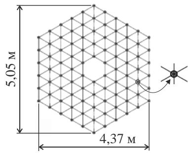 Fig. 7: The initial dimensions of the hexagonal truss structure Using modal analysis, we will verify the truss and beam models for the presence of "rigid body" displacements. Fig. 8 shows the visualization of the first mode of natural vibrations of these models.  Panel label: a.  b Puc. 8: The first natural mode of vibration: a — truss FE; b — beam FE As can be seen, the regular lattice modeled by truss finite elements is kinematically changeable, as it allows for the rotation of rigid platforms. Therefore, in the future study, we will use only beam finite elements. It is necessary to understand that the transformation process from the position where the coordinates of all nodes are equal to 0 will not lead to the expected rise of the rod lattice, i.e., it is necessary to "start" (begin the transformation) with a pre-prepared dome-like geometry (Fig. 9). Let's take the "starting" rise of the arrow $\Delta u_{z} = 0,1\mathrm{m}$. 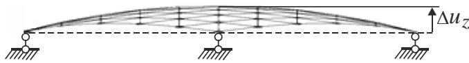 Fig. 9: The "starting" position of the hexagonal rod structure Let's analyze the kinematic shape change for the considered rod structure in the "starting" position, with discrete displacements of the contour nodes in the direction of the X and Y axes (Fig. 10). We assume that the steps for displacements $\Delta x$ and $\Delta y$ are synchronous and equal to $0.01\mathrm{m}$. Fig. 11 shows the visualization of the structure's shape after 50 steps. The rise at the central point after the completion of the transformation was $0.92\mathrm{m}$. The point diagrams of the changes in the longitudinal deformation in the lattice rods $\varepsilon = \Delta l / l$, where $\Delta l$ is the change in the rod length, and $l$ is the initial rod length, with discrete displacements along the X and Y axes, are shown in Fig. 12. 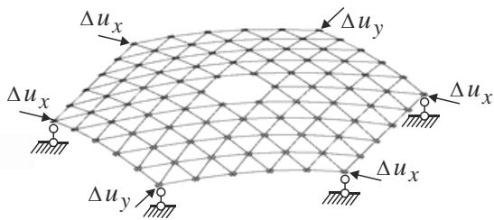 Fig. 10: Discrete displacements along the X and Y axes  Fig. 3: Model of the balloon deformed by a point force [7]   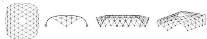 Fig. 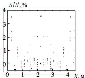11: Visualization of the shape change after 50 steps of displacements along the X and Y axes  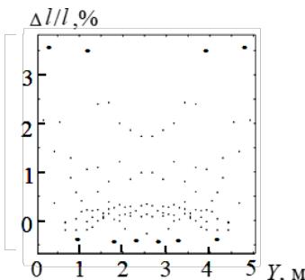 Fig. 12: Point diagrams of changes in the criterion in the rods with displacement of the contour nodes along the X and Y axes From the graphs shown in Fig. 12, it is evident that the most heavily loaded members under the given transformation scheme will be the struts adjacent to the boundary nodes. In physical terms, the extreme value of $\Delta l / l = 3.5\%$ corresponds to a member elongation of $\Delta l = 0.4 \cdot 0.035 = 0.014 \mathrm{~m}$ (14 mm). Naturally, such an axial deformation exceeds the limits of linear theory, and for the corresponding truss members in the actual structure, it is necessary to provide compensators to accommodate this excessive elongation. For this purpose, telescopic compensators with unidirectional collet grips would be a suitable solution. The results of a similar problem solved using the nonlinear solver of the ANSYS Mechanical suite are presented in Fig. 13. In this case, the initial position of the truss was also used, and kinematic boundary conditions in the form of simultaneous displacements of the boundary nodes of $0.5\mathrm{m}$ were applied. The calculations were performed considering large displacements (Large Displacement Static). Comparing the deformed configurations of the truss shown in Figs. 11 and 13, we establish their qualitative agreement. However, the value of the maximum rise $f_{\max} = 0.79\mathrm{m}$ during the simultaneous transformation is lower than the $f_{\max} = 0.92\mathrm{m}$ observed in the case of discrete shape change. Furthermore, there is a significant qualitative and quantitative difference in the distribution of axial strains in the truss members. In particular, the extreme value of $\varepsilon$ in the case of discrete shape change is more than an order of magnitude greater than the corresponding value shown in Fig. 13. 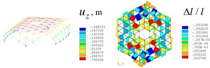 Fig. 13: Solution results using a nonlinear solver: $u_{z}$ - vertical movements; $\varepsilon$ - longitudinal deformation. In summary, when modeling the transformation process of a regular lattice system, the proposed methodology of discrete shape change should be employed, combined with stepwise adjustment and reconstruction of the finite element mesh, taking into account the obtained nodal displacements. This approach is preferable over the use of a single, simultaneous transformation, as it allows for a more accurate capture of the complex deformation behavior of the truss structure. The transformation scheme of a hexagonal truss structure with discrete displacements of $\Delta u_{x} = 0,01\mathrm{mm}$ only along the X-axis is considered (Fig. 14). 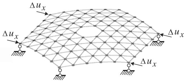 Fig. 14: Discrete displacements along the X axis The visualization of the truss configuration after 50 transformation steps is shown in Fig. 15. In this case, the rise at the pole point after the completion of the transformation was $1.3\mathrm{m}$. The corresponding point diagrams of the axial deformations in the members are presented in Fig. 16. 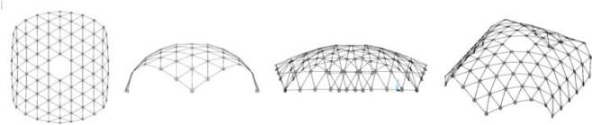 Fig. 15: The visualization of the truss configuration after 50 transformation steps along the X axis 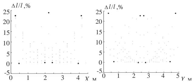 Fig. 16: The corresponding point diagrams of the axial deformations in the members Comparing the dome-shaped forms of the truss structure under uniform compression along the X and Y axes (Fig. 11) and compression only in the X direction (Fig. 14), we conclude that the latter case exhibits a greater degree of surface curvature. However, the maximum value of the ratio $\Delta l / l$ Fig. 16 is almost seven times higher than the similar value presented in the graphs of Fig. 12. As the next example, we will investigate the kinematic shape change of a rectangular regular truss structure, as shown in Fig. 17. 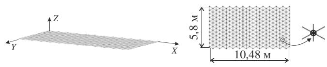 Fig. 17: Initial dimensions of the rectangular truss structure The initial configuration of this truss structure is shown in Fig. 18. In this case, we assume $\Delta u_{z} = 0,5\mathrm{m}$. The scheme of the 4-node kinematic loading is presented in Fig. 19. Here, $\Delta u_{x} = 0,05\mathrm{m}$. 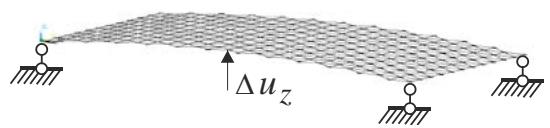 Fig. 18: "Initial" position of the rectangular truss structure 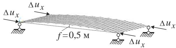 Fig. 19: Scheme of 4-node kinematic loading The visualization of the truss configuration after 50 and 100 transformation steps is shown in Figs. 20 and 21, respectively, while the corresponding point diagrams of $\Delta l / l$ are presented in Figs. 22 and 23.   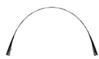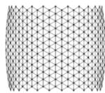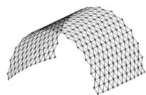 Fig. 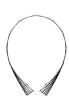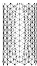20: Visualization of the shape transformation after 50 displacement steps along the X-axis   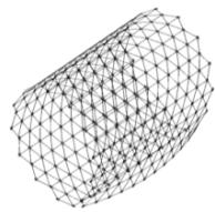 Fig. 21: Visualization of the shape transformation after 100 displacement steps along the X-axis Comparing the diagrams in Figs. 22 and 23, we observe that the largest axial forces in the truss members occur during the initial stage of the transformation. With further deformation of the truss, the increase in the parameter $\Delta l / l$ is approximately $1.5\%$. 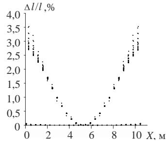 Fig. 22: Diagram (50 steps) 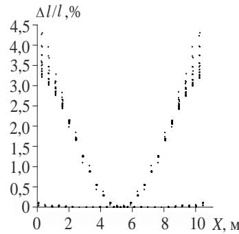 Fig. 23: Diagram (100 steps)  Figure 24 presents the truss configuration under "rigid" two-sided transformation (50 steps). Fig. 24: Visualization of the shape transformation of the truss under "rigid" displacement along the X-axis The diagram of $\Delta l / l$ for the "rigid" transformation scheme of the truss is shown in Fig. 25. 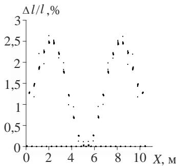 Fig. 25: Diagram of $\Delta l / l$ for "rigid" displacement Comparing the results, at the same number of transformation steps, the amplitude values of the parameter in Fig. 25 are about $1\%$ lower than the corresponding values shown in Fig. 22. ## IV. DISCUSSION AND CONCLUSIONS A finite element modeling methodology has been developed for the transformation of a regular truss system from a planar to a dome-like configuration through the discrete displacement of the boundary nodes of the truss. As a limiting criterion for the structural shape transformation process, the magnitudes of the axial strains in the truss members have been proposed.

Generating HTML Viewer...