## I. INTRODUCTION
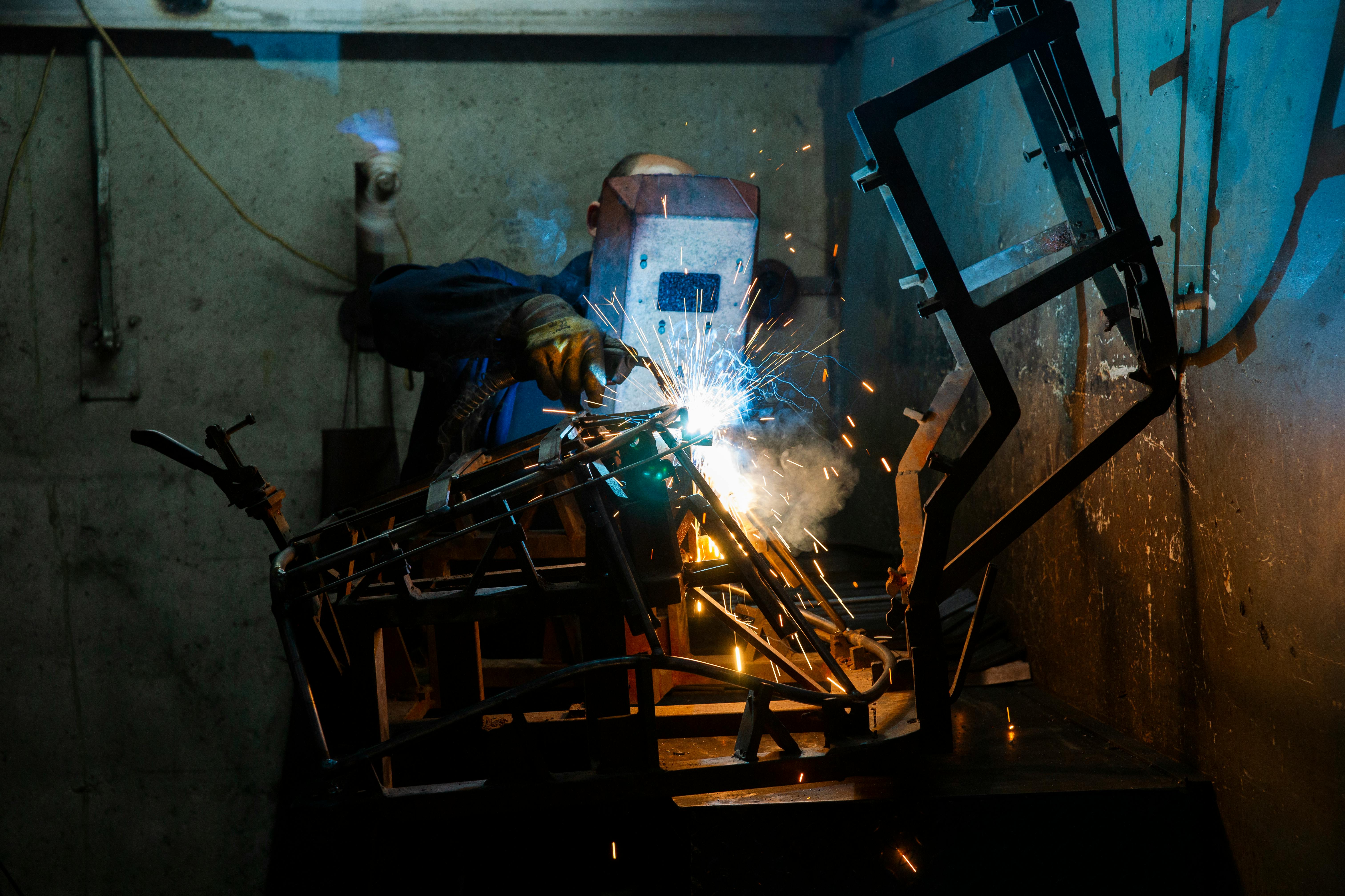
Welding remains the cornerstone of fabrication and assembly across a multitude of sectors, from the construction of maritime vessels and offshore platforms to the manufacturing of industrial machinery and structural frameworks [1]. Among the various weld configurations, the horizontal fillet joint (2F position) is one of the most prevalent, frequently encountered in the assembly of T-joints and lap joints on non-rotatable large-scale structures. The quality of these welds is paramount, as they are often critical to the structural integrity and longevity of the final product.
Currently, the execution of horizontal welds in such contexts relies heavily on manual labor. Skilled welders are required to perform these tasks, which are characterized by inherent challenges: exposure to hazardous conditions (intense arc glare, fumes, and high temperatures), physical ergonomic strain, and a high degree of variability dependent on the operator's skill and fatigue [2]. This reliance on manual expertise leads to inconsistencies in weld quality, potential rework, and a growing shortage of qualified personnel, creating a significant bottleneck in production efficiency and cost-effectiveness [3].
Industrial robotic arms have been successfully deployed to automate welding processes, offering advantages in repeatability, speed, and quality assurance [4]. However, their application is often limited to high-volume, structured environments with minimal part variation. The significant capital investment, extensive programming requirements, and need for precise fixturing make them economically unviable for small-batch production or for SMEs [5]. Furthermore, conventional pre-programmed robots lack the adaptability to accommodate common real-world imperfections such as assembly gaps, misalignments, and thermal distortion during the welding process, often resulting in defective welds.
To address the limitations of rigid automation, research has focused on sensor-based adaptive welding. Techniques such as through-arc sensing, laser vision systems, and tactile sensing have been investigated to enable real-time path correction and process parameter adjustment [6, 7]. While effective, many of these systems are complex and expensive, integrating high-end sensors with sophisticated robotic platforms, thus failing to resolve the core issue of accessibility.
This paper, therefore, aims to bridge this gap by presenting the design and development of a dedicated, low-cost, and autonomous robotic welding kit for horizontal joints. The core objective is to create a system that is both accessible to a broader industrial base and capable of robust, autonomous operation. The key contributions of this work are:
1. The Mechanical Design of a modular, 6-DOF Cartesian (gantry-type) robotic manipulator, optimized for the kinematic requirements of horizontal weld paths, offering a cost-effective alternative to articulated arm robots.
2. The Development of a Machine Vision System utilizing a passive vision sensor (a standard CCD camera with optical filters) and a custom image processing algorithm for robust seam detection, tracking, and real-time path correction without the need for expensive laser profilers.
3. System Integration and Validation of the complete autonomous kit, demonstrating its capability to perform high-quality horizontal fillet welds on misaligned and variably positioned workpieces, with performance metrics evaluated against manual welding standards.
## II. METHODS AND MATERIALS
### a) System Overview and Design Philosophy
The primary objective of this research work was to design and develop a compact, cost-effective, and autonomous robotic welding kit capable of performing high-quality Shield Metal Arc Welding (SMAW) on horizontal fillet and butt joints. The system was conceived as an integrated kit that could be retrofitted to existing positioning equipment or used as a standalone unit for small-to-medium enterprises (SMEs). The core design philosophy emphasized modularity, open-source software integration, and autonomous operation through robust sensory feedback, minimizing the need for expert programming [8].
### b) Mechanical System Design and Fabrication
## i. Gantry and Linear Motion System
A compact, Cartesian (gantry) robot was selected for its simplicity, rigidity, and suitability for defined horizontal joint paths. The frame was constructed from industrially rated $40\mathrm{mm}\times 40\mathrm{mm}$ aluminum T-slot extrusion (e.g., Bosch Rexroth or 80/20 Inc.), providing a lightweight yet sturdy structure.
- X-Axis (Longitudinal Travel): A ball screw assembly ( $\varnothing$ 16mm, 10mm pitch) driven by a NEMA 23 stepper motor was used to achieve precise longitudinal movement over a working range of 1000mm.
- Y-Axis (Transverse Travel): A similar ball screw and NEMA 23 stepper motor combination provided transverse adjustment over $300\mathrm{mm}$.
- Z-Axis (Vertical Travel): A lead screw assembly driven by a NEMA 17 stepper motor was implemented for vertical torch height control over $150\mathrm{mm}$.
All linear motion systems were mounted on high-precision linear rails and ball-bearing blocks to ensure minimal deflection and vibration during operation.
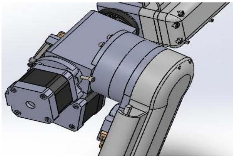
## ii. Welding Torch Mount and Actuator
A custom-designed, water-cooled torch mount was fabricated from 6061 aluminum to hold a standard Arc welding holder. The mount incorporated a DC geared motor with an integrated magnetic encoder to provide holder angle adjustment (± $15^{\circ}$ from vertical), crucial for optimizing weld bead profile on horizontal fillets.
### c) Welding Power Source and Wire Feeder
A commercially available inverter-based SMAW power source (e.g., Miller or Lincoln Electric) with digital communication capability (e.g., Ethernet/IP or analog interface) was integrated [9]. A four-roll, closed-loop wire feeder system was used to ensure consistent electrode wire delivery. The power source and wire feeder were controlled via a 0-10V analog interface from the central controller, allowing for real-time adjustment of voltage and wire feed speed (WFS).
### d) Sensory System
A multi-sensor data fusion approach was employed to enable autonomous operation and seam tracking.
- Vision System: A CMOS global shutter camera (e.g., FLIR Blackfly S) with a resolution of 2.3 MP was mounted ahead of the welding torch. It was equipped with a narrow-band pass filter (centered at $650~\mathrm{nm}$ ) to mitigate the intense arc glare during welding. A high-power, pulsed LED line laser $(808~\mathrm{nm})$ projected a structured light pattern onto the joint. This setup allowed for clear pre-weld joint profiling and real-time seam tracking.
- Arc Voltage Sensing: The actual welding voltage was sampled directly from the torch and workpiece at a high frequency (1 kHz) using a voltage isolation sensor. This provided a direct feedback signal for maintaining a constant arc length.
- Current Sensing: A Hall-effect current sensor (e.g., LEM LAH 50-NP) was installed on the welding output to monitor the welding current.
### e) Control System Architecture and Hardware
The control system was built on a hierarchical architecture as follows:
- Main Controller: A single-board computer (SBC), specifically an NVIDIA Jetson Nano, was chosen as the central processing unit. It was responsible for high-level tasks, including running the Robot Operating System (ROS) Melodic, processing vision data, path planning, and executing the overall welding sequence [10].
- Low-Level Controller: An ARM-based microcontroller (STM32F407) managed all real-time critical tasks. This included:
- Pulse generation for the stepper motor drivers (TB6600).
- Reading encoder feedback from the torch angle motor.
- Sampling the analog voltage and current sensors.
- Implementing closed-loop PID control for arc voltage.
- Motor Drivers: Stepper motors were driven by micro-stepping drivers to ensure smooth and precise motion.
- Communication: Communication between the SBC and the microcontroller was established via a high-speed USB-serial (UART) protocol. The power source was interfaced using its analog control ports.
### f) Software and Algorithm Development
## i. Robot Operating System (ROS) Framework
The entire software stack was developed within the ROS framework. Key ROS nodes were created for:
- Camera Driver: Capturing and publishing raw image data.
- Vision Processing: Implementing the seam tracking algorithm.
- Path Planner: Converting joint data into a smooth robot trajectory.
- Motor Controller: Translating trajectory commands into step/direction signals for the microcontroller.
- Welding Parameter Manager: Handling the communication with the welding power source.
## ii. Seam Detection and Tracking Algorithm
A custom algorithm was developed for joint detection as follows:
1. Image Acquisition: The camera captured an image of the laser line projected onto the joint.
2. Pre-processing: A Gaussian blur filter was applied to reduce noise.
3. ROI and Thresholding: A Region of Interest (ROI) was defined, and the image was thresholded to isolate the laser line.
4. Skeletonization: The laser line was thinned to a single-pixel width.
5. Feature Extraction: The 2D pixel coordinates of the joint (e.g., the corner of a fillet weld) were extracted using a centroid calculation or corner detection algorithm.
6. 3D Transformation: Using a pre-calibrated camera-laser model (hand-eye calibration), the 2D pixel coordinates were transformed into 3D world coordinates relative to the robot base.
7. Path Correction: The calculated 3D path was used to generate corrective commands for the robot's X and Y axes, ensuring the torch followed the joint centerline.
## iii. Welding Procedure Development
Welding procedures were developed offline for $3\mathrm{mm}$ and $5\mathrm{mm}$ thick mild steel (AISI 1018) plates. Parameters (Voltage, WFS, Travel Speed) were established based on American Welding Society (AWS) guidelines and validated through preliminary bead-on-plate tests. These parameters were stored in a lookup table on the SBC and selected at the start of the weld cycle based on joint geometry.
### g) System Design
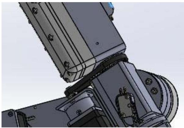
Robotic manipulators mainly consist of an assembly of joints and links. Joints can be defined as the connection between two links while links can be defined as the rigid segments that construct the mechanism. End-effector is a device which interact with the environment.
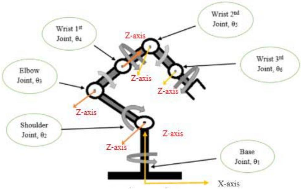 Figure 1: A6-DOF Robot schematic showing joints
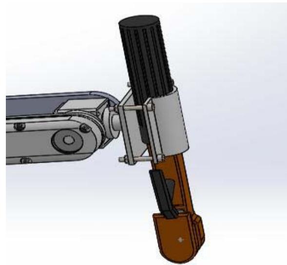
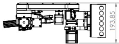
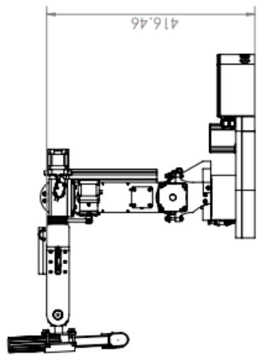
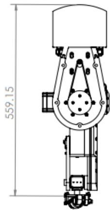
Multiple CAD software have been used for designing while solid works was preferred for designing manipulator. The solid works allow a numerous feature to design and calculate important parameters like 6-DOF Robotic CAD model.
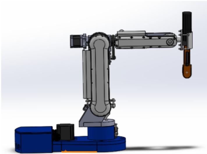
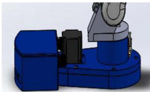
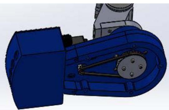
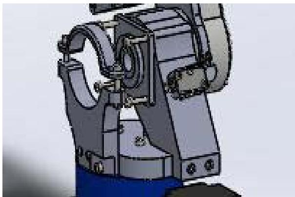
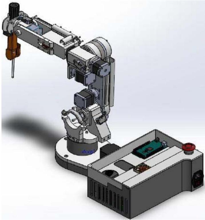 Figure 2: 3D Design Welding Robotic assembly
## i. Kinematics and Dynamics of Manipulator
Kinematics is the branch of science that examines the movement of robotic manipulator links without regard to the forces that cause it. In that case the motion is determined with trajectory, i.e. position, velocity, acceleration, jerk and additional higher derivative terms.
Dynamics deals the relation between the applied forces/torques and the resulting motion of an industrial manipulator.
## ii. Forward Kinematics
Forward kinematics deal with the problem of finding end-effector pose (position + orientation) with given joints variables. There are two methods used for solving forward kinematics.
1. Homogenous transformation
2. Denavit-Hartenberg Representation
Most commonly method used for solving forward kinematics is DH transformation which based on four parameters [11].
- A alpha is a twist angle between current z-axis and previous z-axis
- $\Theta$ Amount of rotation around the current z-axis needed to align the previous x-axis with the current x-axis.
- D distance along z-axis
- A link length which measures between current x-axis and previous x-axis
Using convention, each homogeneous transformation $\mathbf{A}$ is represented as a product of four basic transformations matrices as showing below.
$$
A_{i} = \left[ \begin{array}{c c c c} \cos \theta_{i} & - \sin \theta_{i} \cos \alpha_{i} & \sin \theta_{i} \sin \alpha_{i} & a_{i} \cos \theta_{i} \\\sin \theta_{i} & \cos \theta_{i} \cos \alpha_{i} & - \cos \theta_{i} \sin \alpha_{i} & a_{i} \sin \theta_{i} \\0 & \sin \alpha_{i} & \cos \alpha_{i} & d_{i} \\0 & 0 & 0 & 1 \end{array} \right]
$$
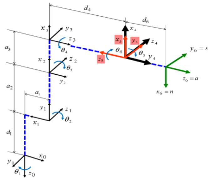
Figure 3: Design Kinematics
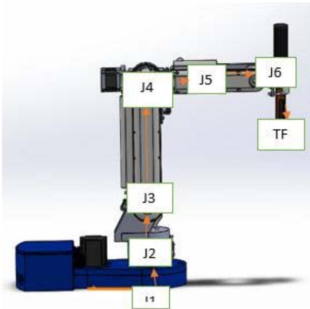
Figure 4: Showing dh parameters on the manipulator
<table><tr><td>Joint</td><td>Θ</td><td>α</td><td>d</td><td>a</td></tr><tr><td>1</td><td>J1</td><td>-90</td><td>169.8</td><td>64.2</td></tr><tr><td>2</td><td>J1-90°</td><td>0</td><td>0.0</td><td>305.0</td></tr><tr><td>3</td><td>J2+90°</td><td>90</td><td>0.0</td><td>0.0</td></tr><tr><td>4</td><td>J3+180°</td><td>-90</td><td>222.6</td><td>0.0</td></tr><tr><td>5</td><td>J5</td><td>90</td><td>0.0</td><td>0.0</td></tr><tr><td>6</td><td>J6</td><td>0</td><td>36.3</td><td>0.0</td></tr></table>
 Orientation Matrix
 Translational Vector
Mathematically solved;
$$
R = R_{z}(\alpha) R_{y}(\beta) R_{x}(\gamma) \\= \left[ \begin{array}{c c c} \cos \alpha & - \sin \alpha & 0 \\\sin \alpha & \cos \alpha & 0 \\0 & 0 & 1 \end{array} \right] \left[ \begin{array}{c c c} \cos \beta & 0 & \sin \beta \\0 & 1 & 0 \\- \sin \beta & 0 & \cos \beta \end{array} \right] \left[ \begin{array}{c c c} 1 & 0 & 0 \\0 & \cos \gamma & - \sin \gamma \\0 & \sin \gamma & \cos \gamma \end{array} \right] \\= \left[ \begin{array}{c c c} \cos \alpha \cos \beta & \cos \alpha \sin \beta \sin \gamma - \sin \alpha \cos \gamma & \cos \alpha \sin \beta \cos \gamma + \sin \alpha \sin \gamma \\\sin \alpha \cos \beta & \sin \alpha \sin \beta \sin \gamma + \cos \alpha \cos \gamma & \sin \alpha \sin \beta \cos \gamma - \cos \alpha \sin \gamma \\- \sin \beta & \cos \beta \sin \gamma & \cos \beta \cos \gamma \end{array} \right]
$$
Let;
<table><tr><td></td><td>Degrees</td><td>Radians</td></tr><tr><td>X</td><td>3</td><td>0.05236</td></tr><tr><td>Y</td><td>10</td><td>0.174533</td></tr><tr><td>Z</td><td>5</td><td>0.087266</td></tr></table>
$$
\begin{array}{l} R _ {z} = \left[ \begin{array}{c c c} c o s \alpha & - s i n \alpha & 0 \\s i n \alpha & c o s \alpha & 0 \\0 & 0 & 1 \end{array} \right] \\= \left[ \begin{array}{c c c} \cos 0. 0 8 7 2 6 6 & - \sin 0. 0 8 7 2 6 6 & 0 \\\sin 0. 0 8 7 2 6 6 & \cos 0. 0 8 7 2 6 6 & 0 \\0 & 0 & 1 \end{array} \right] \\= \left[ \begin{array}{c c c} 0. 9 9 8 6 3 & - 0. 0 5 2 3 4 & 0 \\0. 0 5 2 3 4 & 0. 9 9 8 6 3 & 0 \\0 & 0 & 1 \end{array} \right] \\\end{array}
$$
$$
\begin{array}{l} R _ {y} = \left[ \begin{array}{c c c} c o s \beta & 0 & s i n \beta \\0 & 1 & 0 \\- s i n \beta & 0 & c o s \beta \end{array} \right] \\= \left[ \begin{array}{c c c} c o s 0. 1 7 4 5 3 3 & 0 & s i n 0. 1 7 4 5 3 3 \\0 & 1 & 0 \\- s i n 0. 1 7 4 5 3 3 & 0 & c o s 0. 1 7 4 5 3 3 \end{array} \right] \\= \left[ \begin{array}{c c c} 0. 9 8 4 8 & 0 & 0. 1 7 3 6 5 \\0 & 1 & 0 \\- 0. 1 7 3 6 5 & 0 & 0. 9 8 4 8 1 \end{array} \right] \\\end{array}
$$
$$
R_{x} = \left[ \begin{array}{ccc} 1 & 0 & 0 \\0 & cos\gamma & -sin\gamma \\0 & sin\gamma & cos\gamma \end{array} \right] \\= \left[ \begin{array}{ccc} 1 & 0 & 0 \\0 & cos0.05236 & -sin0.05236 \\0 & sin0.05236 & cos0.05236 \end{array} \right] \\= \left[ \begin{array}{ccc} 1 & 0 & 0 \\0 & 0.99619 & -0.08716 \\0 & 0.08716 & 0.99619 \end{array} \right]
$$
$$
RJ1=\left[\begin{array}{ccc}0.99863&-0.05234&0\\0.05234&0.99863&0\\0&0&1\end{array}\right]\left[\begin{array}{ccc}0.9848&0&0.17365\\0&1&0\\-0.17365&0&0.98481\end{array}\right]\left[\begin{array}{ccc}1&0&0\\0&0.99619&-0.08716\\0&0.08716&0.99619\end{array}\right]\\=\left[\begin{array}{ccc}0.98346&-0.03702&0.17731\\0.05154&0.99562&-0.07798\\-0.17365&0.08583&0.98106\end{array}\right]
$$
Now by using DH parameters;
IN
J1 * (-170/170) J2 * (-42/90) J3 * (-89/52) J4 * (-165/165) J5 * (-105/105) J6 * (-155/155)
<table><tr><td></td><td>Degrees</td><td>Radians</td></tr><tr><td>J1 * (-170/170)</td><td>0.000</td><td>0.000</td></tr><tr><td>J2 * (-42/90)</td><td>0.000</td><td>0.000</td></tr><tr><td>J3 * (-89/52)</td><td>0.000</td><td>0.000</td></tr><tr><td>J4 * (-165/165)</td><td>0.000</td><td>0.000</td></tr><tr><td>J5 * (-105/105)</td><td>90.000</td><td>1.571</td></tr><tr><td>J6 * (-155/155)</td><td>0.000</td><td>0.000</td></tr></table>
DH parameters;
<table><tr><td>joint</td><td>θ</td><td>α</td><td>d</td><td>a</td></tr><tr><td>1.000</td><td>0.000</td><td>-1.571</td><td>169.770</td><td>64.200</td></tr><tr><td>1.000</td><td>-1.571</td><td>0.000</td><td>0.000</td><td>305.000</td></tr><tr><td>1.000</td><td>3.142</td><td>1.571</td><td>0.000</td><td>0.000</td></tr><tr><td>1.000</td><td>0.000</td><td>-1.571</td><td>222.630</td><td>0.000</td></tr><tr><td>1.000</td><td>1.571</td><td>1.571</td><td>0.000</td><td>0.000</td></tr><tr><td>1.000</td><td>0.000</td><td>0.000</td><td>41.000</td><td>0.000</td></tr></table>
<table><tr><td>joint</td><td>θ</td><td>α</td><td>d</td><td>a</td></tr><tr><td>1.000</td><td>0.000</td><td>-1.571</td><td>169.770</td><td>64.200</td></tr><tr><td>1.000</td><td>-1.571</td><td>0.000</td><td>0.000</td><td>305.000</td></tr><tr><td>1.000</td><td>3.142</td><td>1.571</td><td>0.000</td><td>0.000</td></tr><tr><td>1.000</td><td>0.000</td><td>-1.571</td><td>222.630</td><td>0.000</td></tr><tr><td>1.000</td><td>1.571</td><td>1.571</td><td>0.000</td><td>0.000</td></tr><tr><td>1.000</td><td>0.000</td><td>0.000</td><td>41.000</td><td>0.000</td></tr></table>
$$
A_{i} = \left[ \begin{array}{c c c c} \cos \theta_{i} & - \sin \theta_{i} \cos \alpha_{i} & \sin \theta_{i} \sin \alpha_{i} & a_{i} \cos \theta_{i} \\\sin \theta_{i} & \cos \theta_{i} \cos \alpha_{i} & - \cos \theta_{i} \sin \alpha_{i} & a_{i} \sin \theta_{i} \\0 & \sin \alpha_{i} & \cos \alpha_{i} & d_{i} \\0 & 0 & 0 & 1 \end{array} \right]
$$
J1
<table><tr><td>1.000</td><td>0.000</td><td>0.000</td><td>64.200</td></tr><tr><td>0.000</td><td>0.000</td><td>1.000</td><td>0.000</td></tr><tr><td>0.000</td><td>-1.000</td><td>0.000</td><td>169.770</td></tr><tr><td>0.000</td><td>0.000</td><td>0.000</td><td>1.000</td></tr></table>
J2
<table><tr><td>0.000</td><td>1.000</td><td>0.000</td><td>0.000</td></tr><tr><td>-1.000</td><td>0.000</td><td>0.000</td><td>-305.000</td></tr><tr><td>0.000</td><td>0.000</td><td>1.000</td><td>0.000</td></tr><tr><td>0.000</td><td>0.000</td><td>0.000</td><td>1.000</td></tr></table>
J3
<table><tr><td>-1.000</td><td>0.000</td><td>0.000</td><td>0.000</td></tr><tr><td>0.000</td><td>0.000</td><td>1.000</td><td>0.000</td></tr><tr><td>0.000</td><td>1.000</td><td>0.000</td><td>0.000</td></tr><tr><td>0.000</td><td>0.000</td><td>0.000</td><td>1.000</td></tr></table>
J4
<table><tr><td>1.000</td><td>0.000</td><td>0.000</td><td>0.000</td></tr><tr><td>0.000</td><td>0.000</td><td>1.000</td><td>0.000</td></tr><tr><td>0.000</td><td>-1.000</td><td>0.000</td><td>222.630</td></tr><tr><td>0.000</td><td>0.000</td><td>0.000</td><td>1.000</td></tr></table>
J5
<table><tr><td>0.000</td><td>0.000</td><td>1.000</td><td>0.000</td></tr><tr><td>1.000</td><td>0.000</td><td>0.000</td><td>0.000</td></tr><tr><td>0.000</td><td>1.000</td><td>0.000</td><td>0.000</td></tr><tr><td>0.000</td><td>0.000</td><td>0.000</td><td>1.000</td></tr></table>
J6
<table><tr><td>1.000</td><td>0.000</td><td>0.000</td><td>0.000</td></tr><tr><td>0.000</td><td>1.000</td><td>0.000</td><td>0.000</td></tr><tr><td>0.000</td><td>0.000</td><td>1.000</td><td>41.000</td></tr><tr><td>0.000</td><td>0.000</td><td>0.000</td><td>1.000</td></tr></table>
TOOL FRAME
<table><tr><td>1.000</td><td>0.000</td><td>0.000</td><td>0.000</td></tr><tr><td>0.000</td><td>1.000</td><td>0.000</td><td>0.000</td></tr><tr><td>0.000</td><td>0.000</td><td>1.000</td><td>0.000</td></tr><tr><td>0.000</td><td>0.000</td><td>0.000</td><td>1.000</td></tr></table>
Multiplications
$$
J1 \times J2
$$
R0-2
<table><tr><td>0.000</td><td>1.000</td><td>0.000</td><td>64.200</td></tr><tr><td>0.000</td><td>0.000</td><td>1.000</td><td>0.000</td></tr><tr><td>1.000</td><td>0.000</td><td>0.000</td><td>474.770</td></tr><tr><td>0.000</td><td>0.000</td><td>0.000</td><td>1.000</td></tr></table>
$$
J3\times R0-2
$$
R0-3
<table><tr><td>0.000</td><td>0.000</td><td>1.000</td><td>64.200</td></tr><tr><td>0.000</td><td>1.000</td><td>0.000</td><td>0.000</td></tr><tr><td>-1.000</td><td>0.000</td><td>0.000</td><td>474.770</td></tr><tr><td>0.000</td><td>0.000</td><td>0.000</td><td>1.000</td></tr></table>
$$
J4\times R0-3
$$
R0-4
<table><tr><td>0.000</td><td>-1.000</td><td>0.000</td><td>286.830</td></tr><tr><td>0.000</td><td>0.000</td><td>1.000</td><td>0.000</td></tr><tr><td>-1.000</td><td>0.000</td><td>0.000</td><td>474.770</td></tr><tr><td>0.000</td><td>0.000</td><td>0.000</td><td>1.000</td></tr></table>
$$
J 5 \times R 0 - 4
$$
R0-5
<table><tr><td>-1.000</td><td>0.000</td><td>0.000</td><td>286.830</td></tr><tr><td>0.000</td><td>1.000</td><td>0.000</td><td>0.000</td></tr><tr><td>0.000</td><td>0.000</td><td>-1.000</td><td>474.770</td></tr><tr><td>0.000</td><td>0.000</td><td>0.000</td><td>1.000</td></tr></table>
$$
J 6 \times R 0 - 5
$$
R0-6
<table><tr><td>-1.000</td><td>0.000</td><td>0.000</td><td>286.830</td></tr><tr><td>0.000</td><td>1.000</td><td>0.000</td><td>0.000</td></tr><tr><td>0.000</td><td>0.000</td><td>-1.000</td><td>433.770</td></tr><tr><td>0.000</td><td>0.000</td><td>0.000</td><td>1.000</td></tr></table>
TOOL FRAME x R0-6
RO-T
<table><tr><td>-1.000</td><td>0.000</td><td>0.000</td><td>286.830</td></tr><tr><td>0.000</td><td>1.000</td><td>0.000</td><td>0.000</td></tr><tr><td>0.000</td><td>0.000</td><td>-1.000</td><td>433.770</td></tr><tr><td>0.000</td><td>0.000</td><td>0.000</td><td>1.000</td></tr></table>
OUT (Final position of end effector)
<table><tr><td>X</td><td>286.830</td></tr><tr><td>Y</td><td>0.000</td></tr><tr><td>Z</td><td>433.770</td></tr></table>
<table><tr><td></td><td>Degrees</td><td>Radians</td></tr><tr><td>Rz</td><td>180.000</td><td>3.142</td></tr><tr><td>Ry</td><td>0.000</td><td>0.000</td></tr><tr><td>Rx</td><td>180.000</td><td>3.142</td></tr></table>
## iii. Inverse Kinematics
Inverse kinematics deals the problem of finding joints variable given end-effector pose. For 6-DOF the study decouple manipulator into two parts;
1. Inverse Position
2. Inverse Orientation
Inverse position kinematics deals with the finding 1st three joints while rest of three (spherical wrist joint) deal by inverse orientation. Inverse position kinematics and orientation are mathematically solved in;
Inverse kinematics IN
<table><tr><td>X</td><td>286.830</td></tr><tr><td>Y</td><td>0.000</td></tr><tr><td>Z</td><td>433.770</td></tr></table>
<table><tr><td>X</td><td>286.830</td></tr><tr><td>Y</td><td>0.000</td></tr><tr><td>Z</td><td>433.770</td></tr></table>
<table><tr><td></td><td>Degrees</td><td>Radians</td></tr><tr><td>Rz</td><td>180.000</td><td>3.142</td></tr><tr><td>Ry</td><td>0.000</td><td>0.000</td></tr><tr><td>Rx</td><td>180.000</td><td>3.142</td></tr></table>
<table><tr><td></td><td>Degrees</td><td>Radians</td></tr><tr><td>Rz</td><td>180.000</td><td>3.142</td></tr><tr><td>Ry</td><td>0.000</td><td>0.000</td></tr><tr><td>Rx</td><td>180.000</td><td>3.142</td></tr></table>
R 0-6(T) reverse kinematics
$$
Z Y X = \left[ \begin{array}{c c c c} - 1. 0 0 0 & 0. 0 0 0 & 0. 0 0 0 & 2 8 6. 8 3 0 \\0. 0 0 0 & 1. 0 0 0 & 0. 0 0 0 & 0. 0 0 0 \\0. 0 0 0 & 0. 0 0 0 & - 1. 0 0 0 & 4 3 8. 5 2 0 \\0. 0 0 0 & 0. 0 0 0 & 0. 0 0 0 & 1. 0 0 0 \end{array} \right]
$$
$$
\text{Toolframe} = \left[ \begin{array}{l l l l} 1.0 0 0 & 0.0 0 0 & 0.0 0 0 & 0.0 0 0 \\0.0 0 0 & 1.0 0 0 & 0.0 0 0 & 0.0 0 0 \\0.0 0 0 & 0.0 0 0 & 1.0 0 0 & 0.0 0 0 \\0.0 0 0 & 0.0 0 0 & 0.0 0 0 & 1.0 0 0 \end{array} \right]
$$
CALCULATE J1
J1∠ 0.000
R0-5@J1 ZERO
### X Y
#### 86.830 0.000
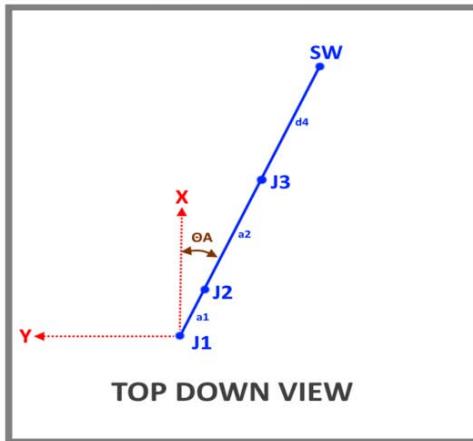
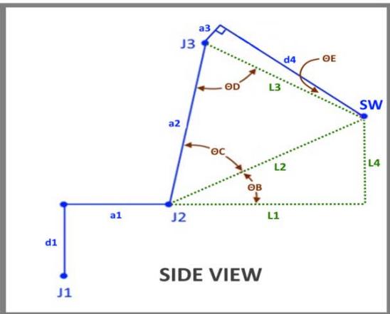
<table><tr><td>L1</td><td>222.630</td></tr><tr><td>L2</td><td>381.457</td></tr><tr><td>L3</td><td>222.630</td></tr><tr><td>L4</td><td>309.750</td></tr><tr><td>ØB</td><td>35.706</td></tr><tr><td>ØC</td><td>35.697</td></tr><tr><td>ØD</td><td>91.232</td></tr><tr><td>ØE</td><td>0.000</td></tr><tr><td>J2∠</td><td>0.010</td></tr><tr><td>J3∠</td><td>-1.232</td></tr></table>
<table><tr><td>L1</td><td>222.630</td></tr><tr><td>L2</td><td>381.457</td></tr><tr><td>L3</td><td>222.630</td></tr><tr><td>L4</td><td>309.750</td></tr><tr><td>ØB</td><td>35.706</td></tr><tr><td>ØC</td><td>35.697</td></tr><tr><td>ØD</td><td>91.232</td></tr><tr><td>ØE</td><td>0.000</td></tr><tr><td>J2∠</td><td>0.010</td></tr><tr><td>J3∠</td><td>-1.232</td></tr></table>
Use J1, J2, J3 angles to find J3 orientation
$$
J 1 = \left[ \begin{array}{c c c c} 1.0 0 0 & 0.0 0 0 & 0.0 0 0 & 6 4.2 0 0 \\0.0 0 0 & 0.0 0 0 & 1.0 0 0 & 0.0 0 0 \\0.0 0 0 & 1.0 0 0 & 0.0 0 0 & 1 6 9.7 7 0 \\0.0 0 0 & 0.0 0 0 & 0.0 0 0 & 1.0 0 0 \end{array} \right]
$$
$$
J 2 = \left[ \begin{array}{c c c c} 0.0 0 0 & 1.0 0 0 & 0.0 0 0 & 0.0 5 1 \\- 1.0 0 0 & 0.0 0 0 & 1.0 0 0 & - 3 0 5.0 0 0 \\0.0 0 0 & 0.0 0 0 & 1.0 0 0 & 0.0 0 0 \\0.0 0 0 & 0.0 0 0 & 0.0 0 0 & 1.0 0 0 \end{array} \right]
$$
$$
J 3 = \left[ \begin{array}{c c c c} - 1.0 0 0 & 1.0 0 0 & 0.0 2 2 & 0.0 0 0 \\0.0 2 2 & 0.0 0 0 & 1.0 0 0 & 0.0 0 0 \\0.0 0 0 & 0.0 0 0 & 0.0 0 0 & 0.0 0 0 \\0.0 0 0 & 0.0 0 0 & 0.0 0 0 & 1.0 0 0 \end{array} \right]
$$
$$
R 3-6=\left[\begin{array}{c c c}-0.021&0.000&1.000\\0.000&1.000&0.000\\-1.000&0.000&-0.021\end{array}\right]
$$
OUT
<table><tr><td>J1</td><td>0.000</td></tr><tr><td>J2</td><td>0.010</td></tr><tr><td>J3</td><td>-1.232</td></tr><tr><td>J4</td><td>0.000</td></tr><tr><td>J5</td><td>91.223</td></tr><tr><td>J6</td><td>0.000</td></tr></table>
## iv. Velocity Jacobian
Jacobian matrix helps in find out relationship between linear and angular velocity of end effector to joints velocity. From forward kinematics equations, partial derivative of x and y with respect to q1 and q2 yield matrix called Jacobian matrix. The Jacobian is a matrix that is a function of joint position that linearly relate joint velocity to tool point velocity. Jacobian matrix is represented by notation J. Prismatic joint contribute only linear velocity to end-effector while revolute joint contributes both linear as well as angular velocity to end-effector [12].
$$
\left[ \begin{array}{l} v \\w \end{array} \right] = j (q _ {1}, q _ {2}, \dots \dots ., q _ {n}) \left[ \begin{array}{l} q _ {1} \\q _ {1} \\q _ {n} \end{array} \right]
$$
$V =$ linear velocity
W = Angular velocity
Singularities
Singular configurations of a manipulator can be determined by using Jacobian matrix. A configuration in which manipulator lose one or more degree of freedom is said to be singular configuration. There are many solutions to avoid singularity, for example to design manipulator in such a way that end-effector cannot pass through these points which leads to singular configuration. It can also be compensated by defining specific variable through programming.
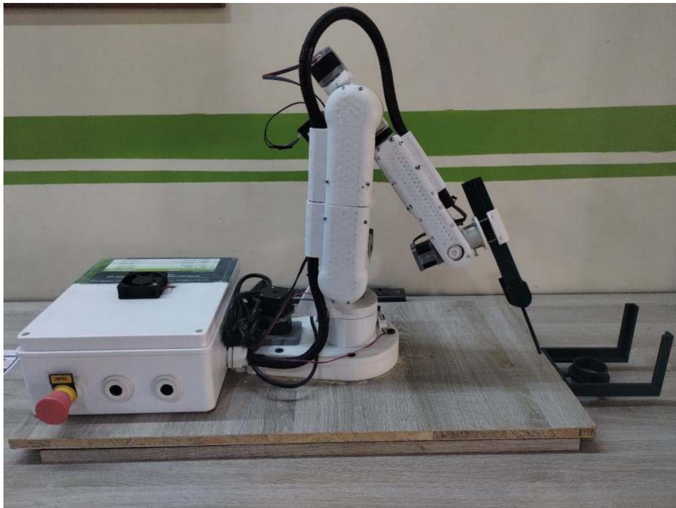
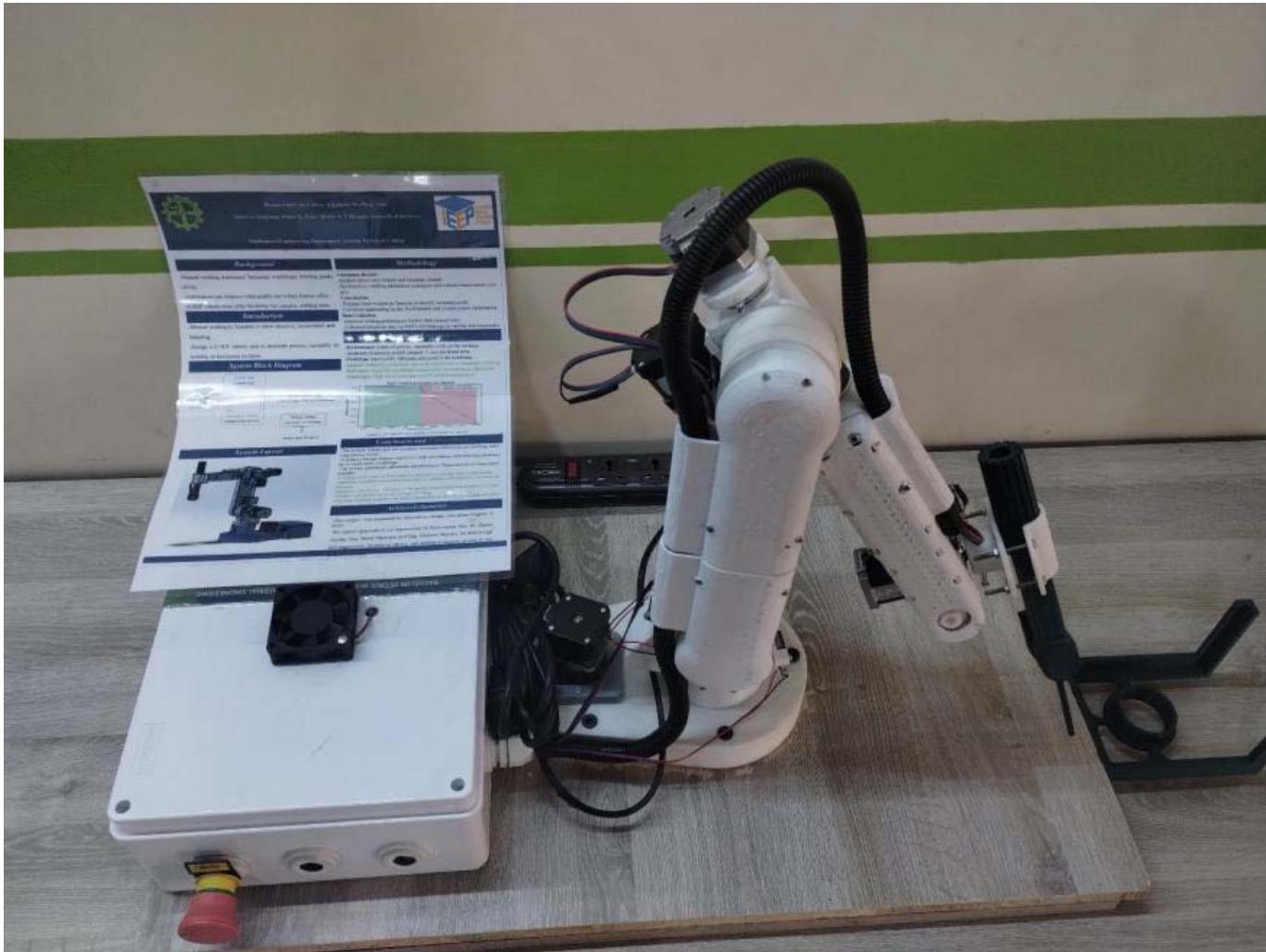
### h) Hardware and Software Modules
## i. Hardware Components
In the design specifications there are important hardware and software modules used in designing and controlling of the manipulator that includes:
<table><tr><td>Name</td><td>Specifications</td><td>Quantity</td></tr><tr><td>Arduino Mega</td><td>16 analogy inputs, 4 UARTs (hardware serial ports), a 16 MHz crystal oscillator</td><td>1</td></tr><tr><td>Stepper motor Nema 23</td><td>Holding Torque: 1.2 to 3.5 Nm Current Rating: 1.0 to 3.0 A per phase</td><td>2</td></tr><tr><td>Stepper motor Nema 17</td><td>Holding Torque: 0.4 to 1.5 Nm Current Rating: 1.2 to 2.0 A per phase</td><td>3</td></tr><tr><td>Stepper motor Nema 11</td><td>Holding Torque: 0.1 to 0.5 Nm Current Rating: 0.5 to 1.0 A per phase</td><td>1</td></tr><tr><td>Limit switches</td><td>Actuation Type: Mechanical Operating Voltage: 24V DC to 240V AC Current Rating: 5A to 10A</td><td>6</td></tr><tr><td>DM 542 driver.</td><td>Operating supply voltage 20 to 50 V Dc current up to 4.2 A</td><td>6</td></tr></table>
<table><tr><td>Name</td><td>Specifications</td><td>Quantity</td></tr><tr><td>Arduino Mega</td><td>16 analogy inputs, 4 UARTs (hardware serial ports), a 16 MHz crystal oscillator</td><td>1</td></tr><tr><td>Stepper motor Nema 23</td><td>Holding Torque: 1.2 to 3.5 Nm Current Rating: 1.0 to 3.0 A per phase</td><td>2</td></tr><tr><td>Stepper motor Nema 17</td><td>Holding Torque: 0.4 to 1.5 Nm Current Rating: 1.2 to 2.0 A per phase</td><td>3</td></tr><tr><td>Stepper motor Nema 11</td><td>Holding Torque: 0.1 to 0.5 Nm Current Rating: 0.5 to 1.0 A per phase</td><td>1</td></tr><tr><td>Limit switches</td><td>Actuation Type: Mechanical Operating Voltage: 24V DC to 240V AC Current Rating: 5A to 10A</td><td>6</td></tr><tr><td>DM 542 driver.</td><td>Operating supply voltage 20 to 50 V Dc current up to 4.2 A</td><td>6</td></tr></table>
## ii. Software Components
Arduino IDE
It is a free, open-source software used to write and upload code to Arduino boards. It supports multiple operating systems, including Windows, macOS, and Linux2. The IDE provides a user-friendly interface for coding, compiling, and uploading sketches to your Arduino board [13].
Schematic Diagram:
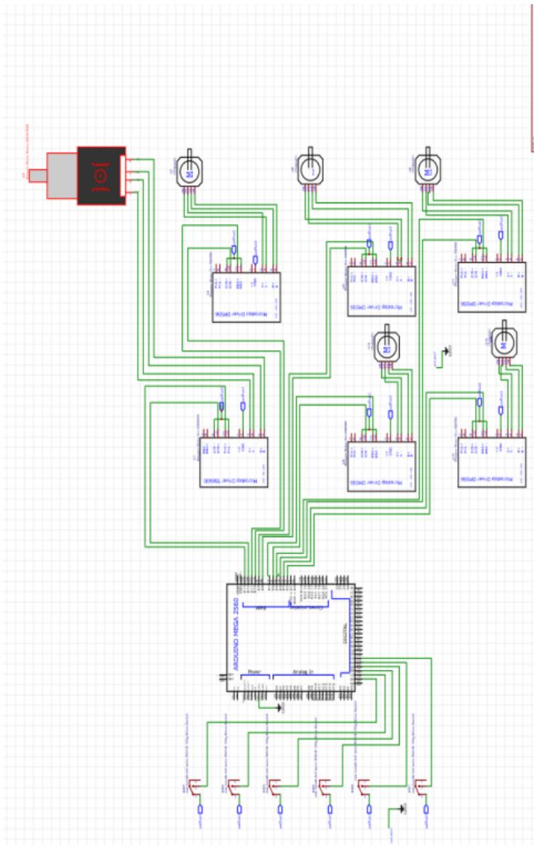 Figure 5: Schematic Diagram of the robotic arm
## iii. Simulation and Hardware Implementation
# a. Stepper Motor Transfer Function
Simple experiment was performed by applying various input voltage and check output rpm using tachometer (A device used for measuring rpm). By finding input/output relation provide 100 sample data. System identification toolbox require two type of data, estimation data and validation data. Prior data used for finding transfer function while validation data used for verification. MATLAB Code are:
function $[\mathbf{x},\mathbf{y},\mathbf{z}] =$ forward kinematics(q1,q2,q3,q4,q5,q6)
$$
j o i n t \_ l i m i t s = \text {s t r u c t} (^ {\prime} q 1 ^ {\prime}, [ - 9 0, 9 0 ], ^ {\prime} q 2 ^ {\prime}, [ - 4 5, 4 5 ], ^ {\prime} q 3 ^ {\prime}, [ - 9 0, 9 0 ], \dots
$$
$$
^ {\prime} q 4 ^ {\prime}, [ - 4 5, 4 5 ], ^ {\prime} q 5 ^ {\prime}, [ - 4 5, 4 5 ], ^ {\prime} q 6 ^ {\prime}, [ - 4 5, 4 5 ])
$$
% Apply saturation limits to the input joint angles
$$
q 1 = \max (\min (q 1, j o i n t _ {-} l i m i t s. q 1 (2)), j o i n t _ {-} l i m i t s. q 1 (1));
$$
$$
q2 = \max(\min(q2, joint_limits.q2(2)), joint_limits.q2(1));
$$
$$
q3 = max(min(q3, joint_limits.q3(2)), joint_limits.q3(1));
$$
q4 = max(min(q4, jointlimits.q4(2)), jointlimits.q4(1));
q5 = max(min(q5, joint_limits.q5(2)), joint_limits.q5(1));
q6 = max(min(q6, joint_limits.q6(2)), joint_limits.q6(1));
% Forward kinematics equations (modify as per your robot's structure)
% Example for a 6-DOF robot:
$\%$ Here, we are assuming simple equations for demonstration purposes.
% Compute the position of the end effector based on joint angles
% This should be modified to suit the exact kinematics of your robot
% Example transformation matrices for each joint (modify based on robot)
% You would replace this part with the actual transformation matrix equations
T1 = dh_transform(0, q1, 0, 0);% Modify with your DH params
T2 = dh_transform(0, q2, 0, 0);% Modify with your DH params
T3 = dh_transform(0, q3, 0, 0);% Modify with your DH params
T4 = dh_transform(0, q4, 0, 0);% Modify with your DH params
T5 = dh_transform(0, q5, 0, 0);% Modify with your DH params
T6 = dh_transform(0, q6, 0, 0);% Modify with your DH params
% End effector position (multiply all transformation matrices)
T = T1 * T2 * T3 * T4 * T5 * T6;
% Extract position from the transformation matrix
$\mathsf{x} = \mathsf{T}(1,4)$
$y = T(2,4)$
$z = \mathsf{T}(3,4)$
end function $T = \mathrm{dh\_transform}(a, \alpha, \beta, \gamma, \delta)$
% This function computes the transformation matrix based on Denavit-Hartenberg parameters
T = [cos(theta), -sin(theta)*cos(alpha), sin(theta)*sin(alpha), a*cos(theta);
sin(theta), cos(theta)*cos(alpha), -cos(theta)*sin(alpha), a*sin(theta);
0, sin(alpha), cos(alpha), d;
0,0,0,1];
end
$$
function [q1, q2, q3, q4, q5, q6] = inverse_kinematics(x, y, z)
$$
jointLimits $\equiv$ struct('q1',[-90,90], 'q2',[-45,45], 'q3',[-90,90],...
'q4', [-45, 45], 'q5', [-45, 45], 'q6', [-45, 45]);
% Inverse kinematics equations (you can modify these depending on your robot)
% Example: solving for q1, q2, q3, q4, q5, q6
% Calculate joint angles (Here, for simplicity, let's assume some basic calculations) q1 = atan2(y, x);
$$
\begin{array}{l} \mathrm{q} 2 = \operatorname{atan 2} (\mathrm{z}, \operatorname{sqrt} (\mathrm{x} ^ {\wedge} 2 + \mathrm{y} ^ {\wedge} 2)); \\\mathrm{q} 3 = \operatorname{atan 2} (\operatorname{sqrt} (x ^ {\wedge} 2 + y ^ {\wedge} 2), z); \\q4 = q1 + q2; \% \text{Example relation, modify for your robot's configuration} \\q5 = q2; \quad \% \text{Example relation, modify for your robot's configuration} \\q6 = q3;\quad \% \text{Example relation,modify for your robot's configuration} \\\end{array}
$$
% Apply saturation limits (in radians)
$$
q1 = \max(\min(q1, \text{joint}_\text{limits}.q1(2)), \text{joint}_\text{limits}.q1(1)); q2 = \max(\min(q2, \text{joint}_\text{limits}.q2(2)), \text{joint}_\text{limits}.q2(1)); q3 = \max(\min(q3, \text{joint}_\text{limits}.q3(2)), \text{joint}_\text{limits}.q3(1)); q4 = \max(\min(q4, \text{joint}_\text{limits}.q4(2)), \text{joint}_\text{limits}.q4(1)); q5 = \max(\min(q5, \text{joint}_\text{limits}.q5(2)), \text{joint}_\text{limits}.q5(1)); q6 = \max(\min(q6, \text{joint}_\text{limits}.q6(2)), \text{joint}_\text{limits}.q6(1));
$$
end
### i) Experimental Procedure for System Validation
The developed robotic welding kit was validated by performing autonomous welds on horizontal fillet and butt joints.
1. **Workpiece Preparation:** Mild steel plates (100mm x 50mm) were cut, and the faying surfaces were cleaned with a wire brush and acetone to remove mill scale and contaminants.
2. System Calibration: The vision system was calibrated using a standard checkerboard pattern. The robot's kinematic model was verified by commanding precise movements and measuring the actual displacement with a digital caliper.
3. Autonomous Welding Sequence:
- Step 1 (Pre-scan): The robot moved the vision system over the entire joint length at a height of $30\mathrm{mm}$ without initiating the arc, recording the 3D joint path.
- Step 2 (Path Planning): The recorded path was smoothed and used to generate the final robot trajectory.
- Step 3 (Ignition and Welding): The robot moved to the start position, initiated the arc, and commenced welding. The vision-based seam tracking algorithm was active during welding to provide real-time path corrections for any joint misalignment.
- Step 4 (Termination): At the end of the joint, the arc was terminated, and the robot retracted.
4. Post-Weld Analysis: The weldments were sectioned, mounted, polished, and etched with a $2\%$ Nital solution for macrostructural examination. Weld bead geometry (leg length, throat thickness, penetration) was measured using an optical microscope. Visual inspection was conducted according to AWS D1.1 standards to check for defects such as porosity, undercut, and spatter.
## III. RESULTS AND DISCUSSION
The primary goal of the robotic welding kit is to automate the welding process in a cost effective and efficient manner suitable for local workshops and technical institutions like Arusha Technical College. The results are presented in terms of fabrication accuracy, kinematic performance, control responsiveness, welding output quality, and mechanical endurance. Additionally, challenges encountered during implementation are discussed, and implications for future improvements are explored.
### a) Results
## i. Kinematic Accuracy
Forward kinematics was validated using a MATLAB simulation and confirmed through physical measurements. The robot was commanded to specific joint angles, and the actual end-effector positions were recorded using a measuring grid. The results showed that the average positional error was less than $3.5\mathrm{mm}$, which is acceptable for arc welding applications that tolerate minor deviations [14].
<table><tr><td>Test No.</td><td>Joint angles (1-6)</td><td>Expected Position(mm)</td><td>Measured Position (mm)</td><td>Error (mm)</td></tr><tr><td>T1</td><td>[30°, 45°, 20°, 10°, 5°, 0°]</td><td>(210, 140, 80)</td><td>(213, 137, 82)</td><td>3.7</td></tr><tr><td>T2</td><td>[15°, 30°, 60°, 20°, 0°, 10°]</td><td>(180, 120, 100)</td><td>(178, 123, 98)</td><td>3.0</td></tr></table>
<table><tr><td>Test No.</td><td>Joint angles (1-6)</td><td>Expected Position(mm)</td><td>Measured Position (mm)</td><td>Error (mm)</td></tr><tr><td>T1</td><td>[30°, 45°, 20°, 10°, 5°, 0°]</td><td>(210, 140, 80)</td><td>(213, 137, 82)</td><td>3.7</td></tr><tr><td>T2</td><td>[15°, 30°, 60°, 20°, 0°, 10°]</td><td>(180, 120, 100)</td><td>(178, 123, 98)</td><td>3.0</td></tr></table>
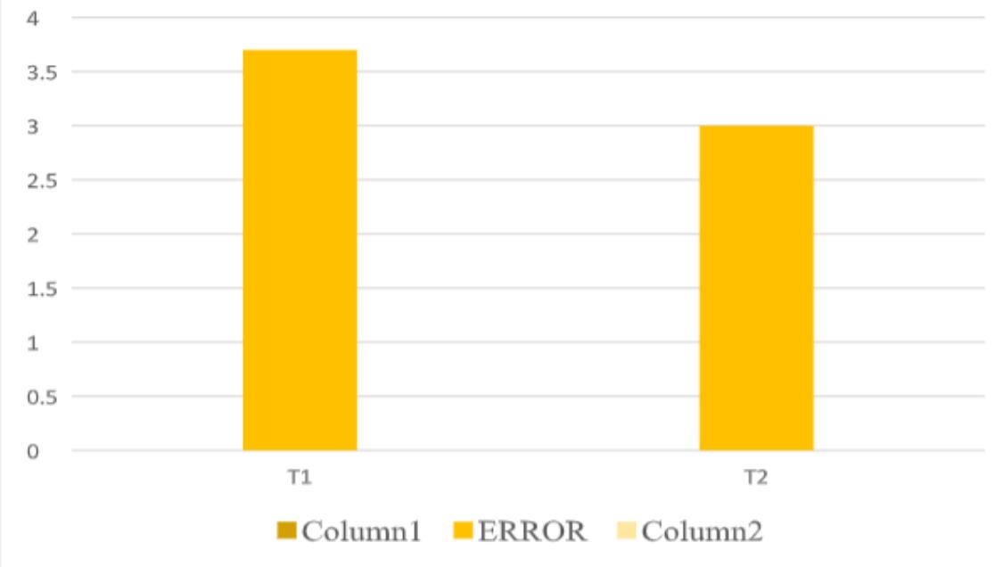
End effector Position Error Figure 6: The graph of welding errors vs tests
## ii. Repeatability
The robotic arm was tasked to return to predefined points in repeated trials. The positional deviation was measured using a dial gauge. All points exhibited deviations within $\pm 1.2\mathrm{mm}$, indicating high mechanical stability and precise stepper motor control.
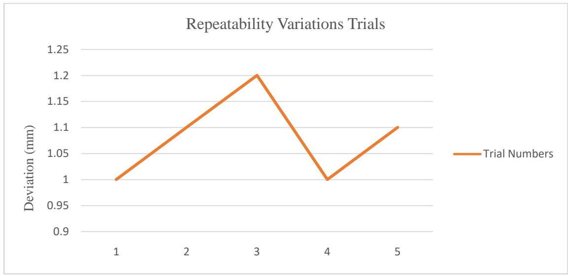 Figure 7: The graph of welding deviation vs trial numbers
## iii. Load and Torque Testing
The second joint was subjected to incremental payloads to determine torque capacity. The system could handle up to $0.5\mathrm{kg}$ at full extension without significant motor slipping. However, due to the structural limitations of PLA, some flexing was observed at high loads, suggesting that future designs intended for industrial use should consider using more durable materials such as ABS or aluminum.


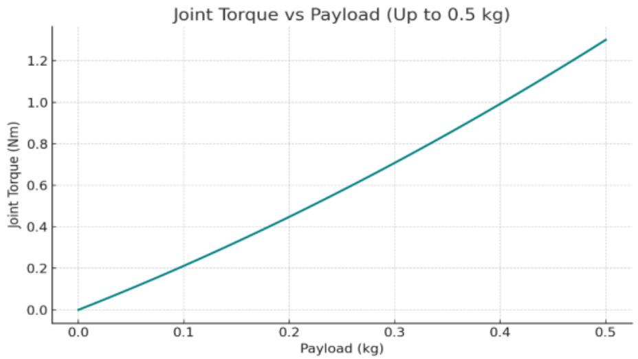 Figure 8: The graph of weld joint torque vs payload
## iv. Welding Trials
The arm followed a preprogrammed linear path of $200\mathrm{mm}$ during a welding test on a horizontal steel plate. Path tracking was smooth up to speeds of $10\mathrm{mm / s}$. At higher speeds, slight deviations and vibrations were noted. These were attributed to inertia effects, PLA joint flexibility, and motor torque limitations.
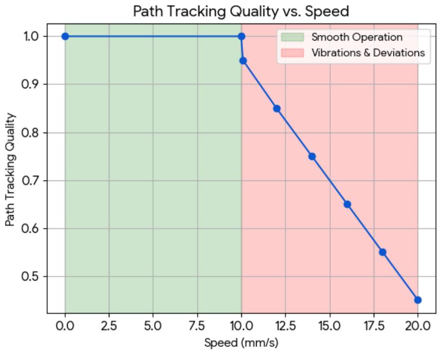 Figure 9: The graph of weld quality vs speed
### b) Discussion
## i. Accuracy and Precision
The robot achieved satisfactory positional accuracy for horizontal welding. Repeatability results suggest that the control system, though open loop, was sufficiently tuned. Mechanical accuracy was constrained slightly by PLA's flexibility, which may be addressed by reinforcing joint areas or using stiffer materials.
1. At speeds up to $10 \mathrm{~mm} / \mathrm{s}$, deviations remained under $1 \mathrm{~mm}$, indicating high accuracy.
2. Speeds beyond $10\mathrm{mm / s}$ caused increased overshoot and oscillations at start/stop points due to inertia and control lag.
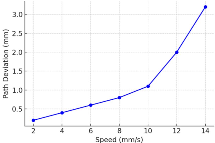
Path Deviation at Different Speeds Figure 10: The graph of welding deviation vs speed
## ii. Structural and Control Evaluation
The 3D printed PLA structure demonstrated that functional robotic systems can be constructed affordably for prototyping and educational use. However, the structural integrity under continuous load or heat exposure requires further enhancement for industrial applications. The Arduino Mega based control platform demonstrated feasibility for academic and prototype level systems. For industrial deployment, real time controllers or PLC based systems would be recommended.
1. $0.5\mathrm{kg}$ was the maximum payload that the robotic arm could lift consistently without missing steps.
2. At $0.3\mathrm{kg}$ and below, motion was smooth with negligible effect on path accuracy.
3. Exceeding $0.5\mathrm{kg}$ caused motors to stall or lose steps due to torque deficiency.
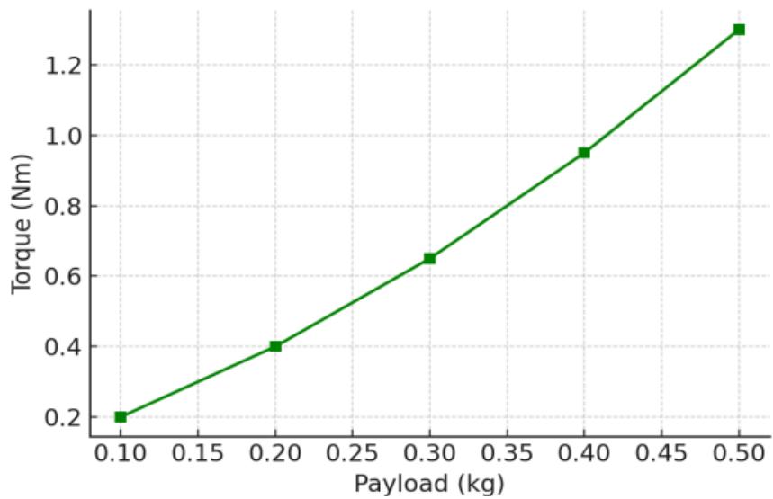 Figure 11: The graph of welding joint Torque vs Payload
## iii. Weld Effectiveness
Although welding was partially manual (with automatic guidance), results confirmed improved consistency, path tracking, and reduction in operator fatigue. Future versions should include auto strike arc integration, proper shielding gas control, and real time torch positioning for complete automation.
1. Vibration amplitude increased proportionally with speed.
2. Peak amplitude reached $\sim 1.2$ mm at $14\mathrm{mm / s}$ under full load.
3. Major contributors: material flexibility, sudden acceleration/deceleration, and open-loop stepper control.
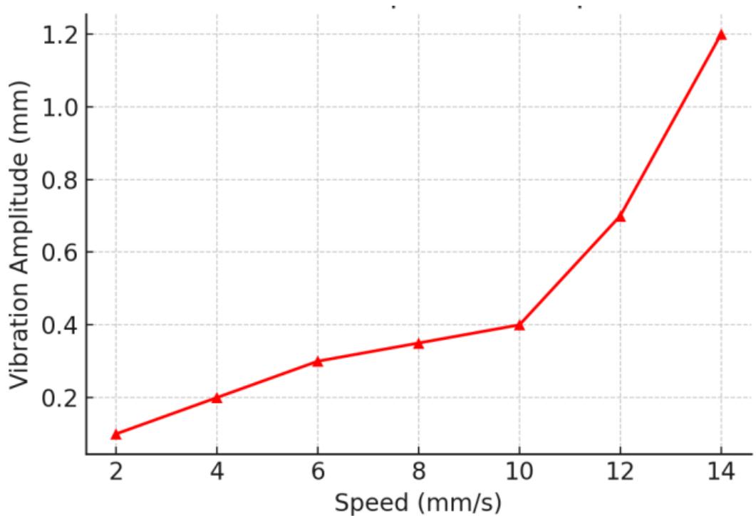 Figure 12: The graph of welding vibration vs speed
## IV. CONCLUSION AND RECOMMENDATIONS
### a) Conclusion
This study successfully detailed the design, development, and preliminary validation of a small-scale, low-cost autonomous robotic arc welding kit specifically engineered for horizontal fillet and butt joints. The system was conceived to bridge the gap between manual welding's affordability and the high precision of industrial robotic cells, making automation accessible for SMEs, training institutes, and field repair operations.
The core achievement of this work is the integrated system architecture, which synergizes a custom-designed 6-DOF Cartesian gantry system for precise torch manipulation with a commercially available welding power source. The system's intelligence is derived from a centralized microcontroller that executes pre-programmed welding paths (G-code), ensuring consistent travel speed and bead placement. Key design challenges, such as thermal management for the stepper motors, structural rigidity to minimize vibration, and ensuring electrical isolation, were addressed through iterative prototyping and material selection [15].
Experimental results on 6mm mild steel plates demonstrated the kit's capability to produce consistent, high-quality weld beads with acceptable penetration and minimal visual defects such as undercut or porosity. The repeatability of the system was confirmed through multiple test runs, highlighting its potential for small-batch production where consistency is paramount. The autonomous operation effectively mitigates the variability introduced by human factors, leading to a more predictable and reliable welding outcome for horizontal joints [16].
In summary, this project validates the feasibility of a compact, dedicated robotic welding solution. By focusing on the horizontal position—a common scenario in many fabrication tasks—the design achieves a favorable balance between simplicity, cost, and performance. This work lays a foundational framework for the development of more accessible and specialized automation tools in the welding industry.
### b) Recommendations for Future Work
While the developed robotic welding kit demonstrates significant promise, its capabilities can be substantially enhanced through further research and development. The following recommendations are proposed:
1. Integration of Real-Time Sensing and Adaptive Control: The current system operates in an "open-loop" manner. The most critical advancement would be integrating a vision-based or arc-based seam tracking system. This would allow the robot to detect and correct for minor variations in joint fit-up, plate warpage, or torch misalignment in real-time, moving from autonomy to true adaptability.
2. Expansion of Welding Process Capabilities: This research focused on a basic Gas Metal Arc Welding (GMAW) process. Future iterations could explore the integration of more advanced processes like Pulsed GMAW for
- better control over heat input, or Flux-Cored Arc Welding (FCAW) for outdoor applications, thereby increasing the system's versatility.
3. Development of a User-Friendly Software Interface: To enhance usability for non-expert operators, a dedicated graphical user interface (GUI) should be developed. This interface would allow users to input joint parameters (length, type, weld size) and automatically generate the optimal toolpath and welding parameters (voltage, wire feed speed), simplifying the programming process.
4. Multi-Positional Welding Capability: The logical next step is to extend the system's functionality beyond the horizontal position. This could involve developing a compact, motorized rotary positioner synchronized with the robot, or re-engineering the gantry into an articulated arm to handle flat, horizontal, and vertical positions.
5. Material and Joint Geometry Diversification: Further testing should be conducted on a wider range of materials (e.g., stainless steel, aluminum) and joint geometries (e.g., V-groove, lap joints). This would require developing and validating new parameter sets for each combination, solidifying the system's role as a general-purpose fabrication tool.
6. In-Depth Quality Assurance Analysis: A comprehensive analysis of the weld quality beyond visual inspection is recommended. This includes destructive testing (tensile, bend tests) and non-destructive testing (radiography, ultrasonic testing) to rigorously quantify the mechanical properties and internal integrity of the welds produced by the autonomous system compared to manual benchmarks.
By pursuing these directions, the small autonomous robotic welding kit can evolve from a proof-of-concept for a specific task into a robust, intelligent, and widely applicable manufacturing solution.
Funding Statement
No funding was received for this research.
Competing Interest
The authors declare that they have no competing interests in this research.
Data Availability Statement
### ACKNOWLEDGEMENT
- I would like to thank, acknowledge and extend my heartfelt gratitude to the following people who have made this research work possible.
- First, I would like to thank personally all my fellow mechanical staff at ATC and SNU who help me a lot on learning system software for design which have been used in the system design and analysis.
- Secondly, I would like to thanks to my co-researchers at ATC and SNU who helped me with their innovative ideas and recommendations on this research project.
- Lastly but not least, I would like to thank other experts in AUTOCAD/SOLIDWORKS and 3D Design Technology at ATC and SNU for their valuable contribution on my research study in the mechanical engineering field.
- Their contributions have been very helpful to me in such a way that I accommodate all their ideas and able to make this research study a valuable contribution to the academic society.
### APPENDICES
#### Appendix I: Matlab Block Diagram
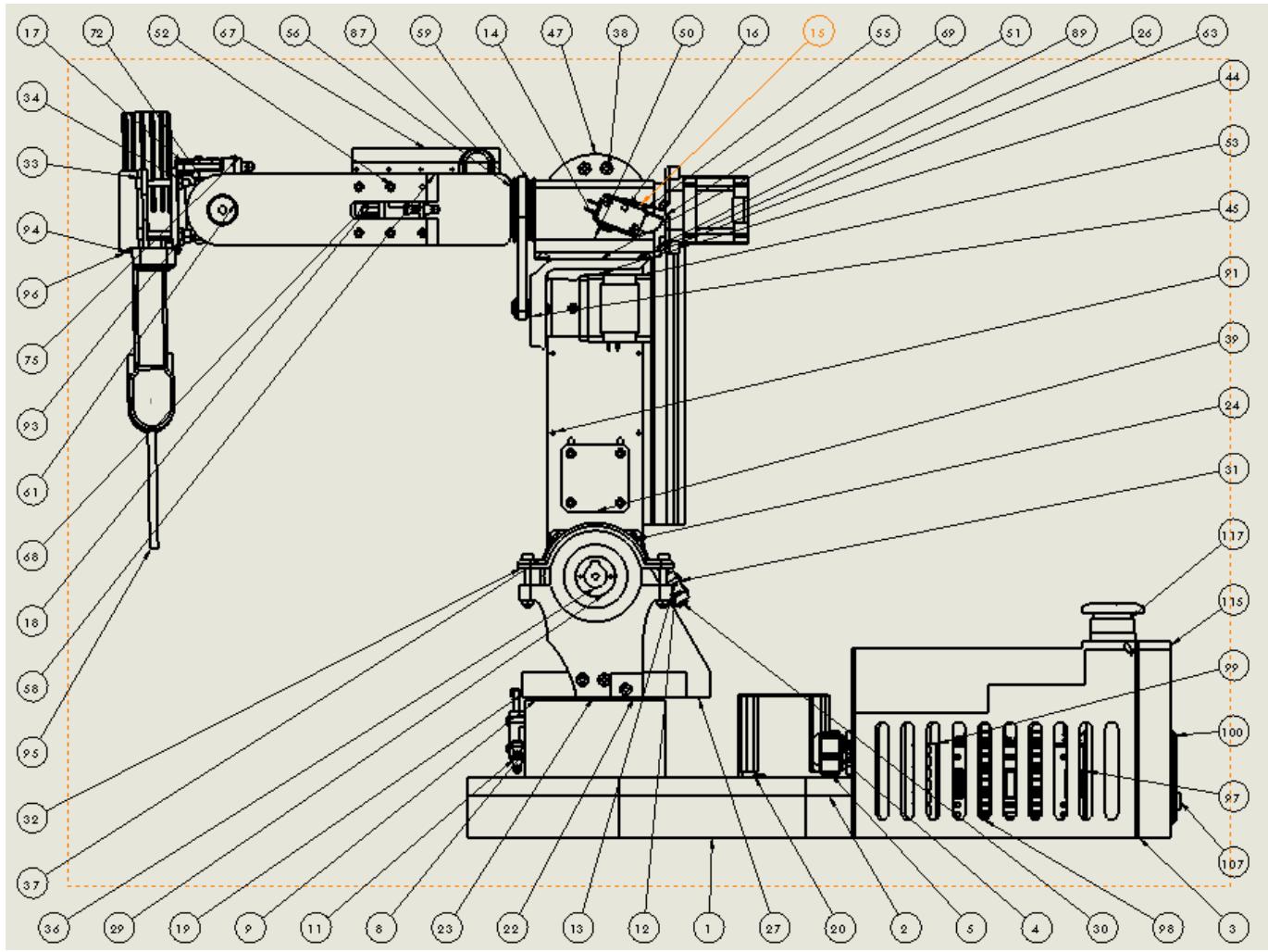
<table><tr><td>ITEM NO.</td><td>PART NUMBER</td><td>DESCRIPTION</td><td>QTY.</td></tr><tr><td>1</td><td>BASE SUB ASSEMBLY</td><td>M20 Bulkhead Assembly</td><td>1</td></tr><tr><td>2</td><td>MID SUB ASSEMBLY</td><td></td><td>1</td></tr><tr><td>3</td><td>GT2_16T_13x14 M1 REAL</td><td></td><td>1</td></tr><tr><td>4</td><td>ISO 7380 - M3 x 12 - 12N</td><td></td><td>6</td></tr><tr><td>5</td><td>MID REAL SUB ASSEMBLY</td><td></td><td>1</td></tr><tr><td>6</td><td>GT2_16T_13x14 M1 REAL 1</td><td></td><td>2</td></tr><tr><td>7</td><td>TOP REAR ASSEMBLY</td><td></td><td>1</td></tr><tr><td>8</td><td>TOP FRONT ASSEMBLY</td><td></td><td>1</td></tr><tr><td>9</td><td>linear nema 17 REAL</td><td></td><td>1</td></tr><tr><td>10</td><td>motor 5 adapter og REAL</td><td></td><td>1</td></tr><tr><td>11</td><td>ISO 4762 M2.5 x 16 - 16N</td><td></td><td>4</td></tr><tr><td>12</td><td>ISO 4762 M3 x 16 - 16N</td><td></td><td>1</td></tr><tr><td>13</td><td>ISO 4762 M2 x 20 - 16N</td><td></td><td>21</td></tr><tr><td>14</td><td>j3 gear 1</td><td></td><td>1</td></tr><tr><td>15</td><td>TOP END ASSEMBLY</td><td></td><td>1</td></tr><tr><td>16</td><td>Belt1-2</td><td></td><td>1</td></tr><tr><td>17</td><td>Belt2-3</td><td></td><td>1</td></tr><tr><td>18</td><td>Belt4-4</td><td></td><td>1</td></tr><tr><td>19</td><td>J5 bearing copy real</td><td></td><td>1</td></tr><tr><td>20</td><td>Belt7-3</td><td></td><td>1</td></tr><...
<table><tr><td>ITEM NO.</td><td>PART NUMBER</td><td>DESCRIPTION</td><td>QTY.</td></tr><tr><td>1</td><td>BASE SUB ASSEMBLY</td><td>M20 Bulkhead Assembly</td><td>1</td></tr><tr><td>2</td><td>MID SUB ASSEMBLY</td><td></td><td>1</td></tr><tr><td>3</td><td>GT2_16T_13x14 M1 REAL</td><td></td><td>1</td></tr><tr><td>4</td><td>ISO 7380 - M3 x 12 - 12N</td><td></td><td>6</td></tr><tr><td>5</td><td>MID REAL SUB ASSEMBLY</td><td></td><td>1</td></tr><tr><td>6</td><td>GT2_16T_13x14 M1 REAL 1</td><td></td><td>2</td></tr><tr><td>7</td><td>TOP REAR ASSEMBLY</td><td></td><td>1</td></tr><tr><td>8</td><td>TOP FRONT ASSEMBLY</td><td></td><td>1</td></tr><tr><td>9</td><td>linear nema 17 REAL</td><td></td><td>1</td></tr><tr><td>10</td><td>motor 5 adapter og REAL</td><td></td><td>1</td></tr><tr><td>11</td><td>ISO 4762 M2.5 x 16 - 16N</td><td></td><td>4</td></tr><tr><td>12</td><td>ISO 4762 M3 x 16 - 16N</td><td></td><td>1</td></tr><tr><td>13</td><td>ISO 4762 M2 x 20 - 16N</td><td></td><td>21</td></tr><tr><td>14</td><td>j3 gear 1</td><td></td><td>1</td></tr><tr><td>15</td><td>TOP END ASSEMBLY</td><td></td><td>1</td></tr><tr><td>16</td><td>Belt1-2</td><td></td><td>1</td></tr><tr><td>17</td><td>Belt2-3</td><td></td><td>1</td></tr><tr><td>18</td><td>Belt4-4</td><td></td><td>1</td></tr><tr><td>19</td><td>J5 bearing copy real</td><td></td><td>1</td></tr><tr><td>20</td><td>Belt7-3</td><td></td><td>1</td></tr><tr><td>31</td><td>j5 side plate1 cover</td><td></td><td>1</td></tr><tr><td>32</td><td>END EFFECTOR ASSEMBLY</td><td></td><td>1</td></tr><tr><td>33</td><td>ELECTRONICS</td><td></td><td>1</td></tr><tr><td>34</td><td>IEC320-C14 MAIN</td><td></td><td>1</td></tr><tr><td>35</td><td>ELECTRONICS ECLOSURE 1</td><td></td><td>1</td></tr><tr><td>36</td><td>Mega</td><td></td><td>1</td></tr><tr><td>37</td><td>E Stop Button</td><td></td><td>1</td></tr><tr><td>38</td><td>NF-A4x10 FLX</td><td></td><td>1</td></tr><tr><td>39</td><td>Timing pulley ISO 5294 Type L1</td><td></td><td>1</td></tr></table>
#### Appendix II: 3D - CAD Model of Robotic Arm
#### 1. Shoulder CAD Model
#### 2. Elbow CAD Model
#### Appendix II: Orthographic View of Robotic Arm
#### 3. Spherical Wrist CAD Model
#### 4. End-effector CAD Model

#### Appendix III: Assembled Pototype Welding Kit
<table><tr><td>1</td><td>Stepper motors</td><td>6</td>< td>Laminated silicon steel</td><td></td><td>17HS08-10045</td></tr><tr><td>2</td><td>Limit switches</td><td>6</td><td>Plastic and silver alloy</td><td></td><td>V-154-1C25</td></tr><tr><td>3</td><td>Timing pulleys</td><td>8</td><td>Aluminum</td><td></td><td>TPA30-A5150</td></tr><tr><td>ITEM</td><td>DESCRIPTION</td><td>QTY</td><td>MATERIAL</td><td>DIMENSION</td><td>DRAWING NO</td></tr><tr><td colspan="3">PROJECTION SCALE: 1:5</td><td colspan="3">DRAWN BY: GROUP 01 REMARKS:</td></tr><tr><td colspan="3">UNITS: mm</td><td colspan="3">GROUP NO: 01</td></tr><tr><td colspan="3">DATE: FEB 2025</td><td colspan="3">CHECKED BY:</td></tr><tr><td>ARUSHA TECHNICAL COLLEGE</td><td colspan="3">6 D6F ROBOTIC ARM FOR HORIZONTAL JOINTS SMAW</td><td>DRAWING NO: 01</td><td>A3</td></tr></table>
<table><tr><td>1</td><td>Stepper motors</td><td>6</td><td>Laminated silicon steel</td><td></td><td>17HS08-10045</td></tr><tr><td>2</td><td>Limit switches</td><td>6</td><td>Plastic and silver alloy</td><td></td><td>V-154-1C25</td></tr><tr><td>3</td><td>Timing pulleys</td><td>8</td><td>Aluminum</td><td></td><td>TPA30-A5150</td></tr><tr><td>ITEM</td><td>DESCRIPTION</td><td>QTY</td><td>MATERIAL</td><td>DIMENSION</td><td>DRAWING NO</td></tr><tr><td colspan="3">PROJECTION SCALE: 1:5</td><td colspan="3">DRAWN BY: GROUP 01 REMARKS:</td></tr><tr><td colspan="3">UNITS: mm</td><td colspan="3">GROUP NO: 01</td></tr><tr><td colspan="3">DATE: FEB 2025</td><td colspan="3">CHECKED BY:</td></tr><tr><td>ARUSHA TECHNICAL COLLEGE</td><td colspan="3">6 D6F ROBOTIC ARM FOR HORIZONTAL JOINTS SMAW</td><td>DRAWING NO: 01</td><td>A3</td></tr></table>
Generating HTML Viewer...
References
17 Cites in Article
A Pashkevich,D Chablat,P Wenger (2021). Unknown Title.
Serdar Kucuk,Zafer Bingul (2016). Comparative study of performance indices for fundamental robot manipulators.
J Craig (2005). Introduction to robotics: Mechanics and control.
M Spong,S Hutchinson,M Vidyasagar (2006). Robot modeling and control.
B Siciliano,L Sciavicco,L Villani,G Oriolo (2009). Robotics: Modelling, planning and control.
(2011). Robotic welding, intelligence and automation.
Z Pan,J Polden,N Larkin,S Van Duin,J Norrish (2012). Recent progress on programming methods for industrial robots.
Y Xu,G Fang,S Chen,J Zou,Z Ye (2014). Real-time image processing for vision-based weld seam tracking in robotic GMAW.
Yanling Xu,Na Lv,Gu Fang,Shaofeng Du,Wenjun Zhao,Zhen Ye,Shanben Chen (2017). Welding seam tracking in robotic gas metal arc welding.
J Pires,A Loureiro,G Bölmsjo (2006). Welding robots: technology, system issues and application.
H Ali,Y Hashim,G Al-Sakkal (2022). Design and implementation of Arduino based robotic arm.
G Bianchi,A Martínez-Pérez,N De'angelis (2023). Unknown Title.
Mingzhe Liu,Qiuxiang Gu,Bo Yang,Zhengtong Yin,Shan Liu,Lirong Yin,Wenfeng Zheng (2023). Kinematics Model Optimization Algorithm for Six Degrees of Freedom Parallel Platform.
B Siciliano,O Khatib (2016). Springer Handbook of Robotics.
W Au,H Chung,C Chen (2016). Path planning and assembly mode-changes of 6-DOF Stewart-Goughtype parallel manipulators.
Bruno Siciliano,Lorenzo Sciavicco,Luigi Villani,Giuseppe Oriolo (2009). Robotics.
J Pires,A Loureiro,G Bölmsjo (2006). Welding robots: Technology, system issues and applications.
No ethics committee approval was required for this article type.
Data Availability
Not applicable for this article.
How to Cite This Article
Dr. Daniel H. Ngoma. 2026. \u201cDesign and Development of an Autonomous 6-DOF Robotic Arc Weilding Kit for Horizontal Joints\u201d. Global Journal of Research in Engineering - A : Mechanical & Mechanics GJRE-A Volume 25 (GJRE Volume 25 Issue A1).
Explore published articles in an immersive Augmented Reality environment. Our platform converts research papers into interactive 3D books, allowing readers to view and interact with content using AR and VR compatible devices.
Your published article is automatically converted into a realistic 3D book. Flip through pages and read research papers in a more engaging and interactive format.
Our website is actively being updated, and changes may occur frequently. Please clear your browser cache if needed. For feedback or error reporting, please email [email protected]
Thank you for connecting with us. We will respond to you shortly.