I. LPI RADAR OVERVIEW

Many users of radar today are specifying Low Probability of Intercept (LPI) as an important tactical requirement [PAC09] [STO13]. The term LPI (whose meaning is not absolutely precise) [SCH06], [WIL06] is that property of a radar that, because of its low power, high duty cycle, ultra-low sidelobes, power management, wide bandwidth, frequency/phase modulation, and other design attributes, makes it difficult to be detected by means of intercept receivers such as electronic support receivers, electronic intelligence receivers, and radar warning receivers [WSQ19]. The goal of the LPI radar is to detect targets at longer ranges than the intercept receiver can detect the LPI radar. It is important to note that defining a radar to be LPI necessitates defining the corresponding intercept receiver. That is, the success of an LPI radar is measured by how hard it is for the intercept receiver to detect and intercept the radar emissions.

One formal definition is as follows: A low probability of intercept (LPI) radar is defined as a radar that uses a special emitted waveform intended to prevent a non-cooperative intercept receiver from intercepting and detecting its emission [PAC09].

The LPI emitter has established itself as the premier tactical and strategic radar in the military spectrum. In addition to surveillance and navigation, the LPI emitter also operates in the time-critical domain for applications such as fire control and missile guidance [WIL06].

II. LPI RADAR CHARACTERISTICS

Some of the characteristics of the LPI radar are power management, ultra-low side lobes, and pulse compression.

Power management is the radar's ability to control the power level so that it emits only the necessary power for detection of a target. An intercept receiver is used to seeing an increase in power as the radar approaches. If a power managed LPI radar decreases the power as it approaches the target, an intercept receiver may incorrectly assume that the radar is not approaching, and therefore that no response management is necessary, which could be a deadly decision [WIL06] [SHC19].

Ultra-low side lobes prevent an intercept receiver from detecting radar emissions from the side lobes of the radar. Ultra-low side lobes are required to be -45dB or lower [SON22].

Pulse compression is another important LPI radar characteristic. For frequency modulation LPI radars, the transmitted Continuous Wave (CW) signal is coded with a reference signal that spreads the transmitted energy in frequency, making it more difficult for an intercept receiver to detect and identify the LPI radar. The reference signal can be a linear frequency modulated signal or an Frequency Shift Keying (FSK) (frequency hopping). The most popular implementation has been the Frequency Modulated Continuous Wave (FMCW) [GUL07], [LIX23].

If the radar uses an FMCW waveform, the processing gain (apart from any noncoherent integration) is the sweep or modulation period $t_m$, multiplied by the sweep (input) bandwidth, $\mathrm{\Delta }F$ (see equation (1)). That is:

The LPI receiver compresses (correlates) the received signal from the target using the stored reference signal, for the purpose of performing target detection. The correlation receiver is a 'matched receiver' if the reference signal is exactly the same duration as the finite duration return signal [PAC09], [WIL06].

III. LPI RADAR WAVEFORMS

This section looks at the FMCW radar waveform.

FMCW is a signal that is frequently encountered in modern radar systems [VGS17]. The frequency modulation spreads the transmitted energy over a large modulation bandwidth $\mathrm{\Delta }F$, providing good range resolution that is critical for discriminating targets from clutter. The power spectrum of the FMCW signal is nearly rectangular over the modulation bandwidth, so non-cooperative interception is difficult. Since the transmit waveform is deterministic, the form of the return signals can be predicted. This gives it the added advantage of being resistant to interference (such as jamming), since any signal not matching this form can be suppressed [WIL06]. Consequently, it is difficult for an intercept receiver to detect the FMCW waveform and measure the parameters accurately enough to match the jammer waveform to the radar waveform [PAC09].

The most popular linear modulation utilized is the triangular modulated FMCW emitter, since it can measure the target's range and Doppler [MIL18]. Triangular modulated FMCW is the waveforms that is employed in this paper.

IV. DETECTION OF LPI RADARS: INTERCEPT RECEIVER OVERVIEW

In this section we switch from the topic of LPI radars, to the topic of those devices that detect and characterize LPI radar signals – intercept receivers.

The three main types of intercept receivers are: electronic support receivers, electronic intelligence receivers, and radar warning receivers.

Electronic intelligence is the result of observing the signals transmitted by radar systems to obtain information about their capabilities: it is the remote sensing of remote sensors. Through electronic intelligence, it is possible to obtain valuable information while remaining remote from the radar itself. Identification is performed by comparing the intercepted signal signature against the signatures contained within its threat library [CLA13]. Clearly, the underlying basic function of electronic intelligence is to determine the capabilities of the radar, so that decisions can be made as to what threat it poses [GRA11]. Electronic intelligence receivers are the least time critical of the three intercept receivers. The outputs of the electronic intelligence receiver may be analyzed using off-line analysis tools based on software.

Radar warning receivers are designed to give nearly immediate warning if specific threat signals are received (e.g., illumination of an aircraft's warning receiver by the target tracking radar of a threatening system). The warning receiver typically has poor sensitivity and feeds into a near-real-time processor that uses a few parameter measurements to identify a threat. Usually, rough direction (e.g., quadrant or octant) is determined for the threat and the operator has a crude display showing functional radar type, direction, and relative range (strong signals displayed as being nearer than weaker ones). This type of receiver does not provide the kind of output that is analyzed using the methods described later in this paper.

Electronic support receivers encompass all actions necessary to provide the information required for immediate decisions involving electronic warfare operations, threat avoidance, targeting, and homing [ASC16], [WIL06].

V. INTERCEPT RECEIVER SIGNAL ANALYSIS TECHNIQUES

This section describes some of the classical time-frequency analysis techniques as well as the reassignment method utilized in this paper.

a) Time-Frequency Analysis

Time-frequency signal analysis concerns the analysis and processing of signals with time-varying frequency content. Such signals are best represented by a time-frequency distribution, which is intended to show how the energy of the signal is distributed over the two-dimensional time-frequency plane [ZML16]. Processing of the signal may then exploit the features produced by the concentration of signal energy in two dimensions (time and frequency), instead of only one dimension (time or frequency) [BOA15]. Since noise tends to spread out evenly over the time-frequency domain, while signals concentrate their energies within limited time intervals and frequency bands; the local SNR of a noisy signal can be improved simply by using time-frequency analysis [BOA15]. Also, the intercept receiver can increase its processing gain by implementing time-frequency signal analysis [GHA20].

As alluded to previously, time-frequency distributions are useful for the visual interpretation of signal dynamics, as an experienced operator can quickly detect a signal and extract the signal parameters by analyzing the time-frequency distribution [BOA15].

b) Scalogram (Wavelet Transform)

The wavelet transform will be examined first, and then connected to the Scalogram. The Scalogram is defined as the magnitude squared of the wavelet transform, and can be used as a time-frequency distribution [BOA15], [SIA21].

The idea of the wavelet transform (equation (2)) is to project a signal $x$ on a family of zero-mean functions (the wavelets) deduced from an elementary function (the mother wavelet) by translations and dilations:

where ${\mathrm{\Psi }}_{t,a}(s)=|a{|}^{-1/2}\mathrm{\Psi }\left(\frac{s-t}{a}\right)$. The variable $a$ corresponds to a scale factor, in the sense that taking dilates the wavelet $\mathrm{\Psi }$ and taking compresses $\mathrm{\Psi }$. By definition, the wavelet transform is more a time-scale than a time-frequency representation. However, for wavelets which are well localized around a non-zero frequency ${\nu }_0$ at a scale $=1$, a time-frequency interpretation is possible thanks to the formal identification $\nu =\frac{{\nu }_0}{a}$.

The wavelet transform is of interest for the analysis of non-stationary signals, because it provides still another alternative to the Short-Time Fourier transform (STFT) and to many of the quadratic time-frequency distributions. The basic difference between the STFT and the wavelet transform is that the STFT uses a fixed signal analysis window, whereas the wavelet transform uses short windows at high frequencies and long windows at low frequencies. This helps to diffuse the effect of the uncertainty principle by providing good time resolution at high frequencies and good frequency resolution at low frequencies. This approach makes sense especially when the signal at hand has high frequency components for short durations and low frequency components for long durations. The signals encountered in practical applications are often of this type.

The wavelet transform allows localization in both the time domain via translation of the mother wavelet, and in the scale (frequency) domain via dilations. The wavelet is irregular in shape and compactly supported, thus making it an ideal tool for analyzing signals of a transient nature; the irregularity of the wavelet basis lends itself to analysis of signals with discontinuities or sharp changes, while the compactly supported nature of wavelets enables temporal localization of a signal's features [HEZ16]. Unlike many of the quadratic functions such as the Wigner-Ville Distribution (WVD) and Choi-Williams Distribution (CWD), the wavelet transform is a linear transformation, therefore cross-term interference is not generated. There is another major difference between the STFT and the wavelet transform;

the STFT uses sines and cosines as an orthogonal basis set to which the signal of interest is effectively correlated against, whereas the wavelet transform uses special 'wavelets' which usually comprise an orthogonal basis set. The wavelet transform then computes coefficients, which represents a measure of the similarities, or correlation, of the signal with respect to the set of wavelets. In other words, the wavelet transform of a signal corresponds to its decomposition with respect to a family of functions obtained by dilations (or contractions) and translations (moving window) of an analyzing wavelet.

A filter bank concept is often used to describe the wavelet transform. The wavelet transform can be interpreted as the result of filtering the signal with a set of bandpass filters, each with a different center frequency [PRL19].

Like the design of conventional digital filters, the design of a wavelet filter can be accomplished by using a number of methods including weighted least squares [WAL13], orthogonal matrix methods [ANS10], nonlinear optimization, optimization of a single parameter (e.g. the passband edge) [GUT22] and a method that minimizes an objective function that bounds the out-of-tile energy [STS16].

Here are some properties of the wavelet transform: 1) The wavelet transform is covariant by translation in time and scaling. The corresponding group of transforms is called the Affine group; 2) The signal $x$ can be recovered from its wavelet transform via the synthesis wavelet; 3) Time and frequency resolutions, like in the STFT case, are related via the Heisenberg-Gabor inequality. However in the wavelet transform case, these two resolutions depend on the frequency: the frequency resolution becomes poorer and the time resolution becomes better as the analysis frequency grows; 4) Because the wavelet transform is a linear transform, it does not contain cross-term interferences [SKZ21].

Since the wavelet transform behaves like an orthonormal basis decomposition, it can be shown that it preserves energy:

where $E_x$ is the energy of $x$. This leads us to define the Scalogram (equation (3)) of $x$ as the squared modulus of the wavelet transform. It is an energy distribution of the signal in the time-scale plane, associated with the measure $\frac{da}{a^2}$.

As is the case for the wavelet transform, the time and frequency resolutions of the Scalogram are related via the Heisenberg-Gabor principle.

The interference terms of the Scalogram, as for the Spectrogram (the squared modulus of the STFT), are also restricted to those regions of the time-frequency plane where the corresponding signals overlap. Therefore, if two signal components are sufficiently far apart in the time-frequency plane, their cross-Scalogram will be essentially zero [STS17].

For this paper, the Morlet Scalogram will be used. The Morlet wavelet is obtained by taking a complex sine wave and localizing it with a Gaussian envelope. The Mexican hat wavelet isolates a single bump of the Morlet wavelet. The Morlet wavelet has good focusing in both time and frequency [YCC14].

c) The Reassignment Method

Bilinear time-frequency distributions offer a wide range of methods designed for the analysis of non stationary signals. Nevertheless, a critical point of these methods is their readability [ZHF22], which means both a good concentration of the signal components along with few misleading interference terms. A lack of readability, which is a known deficiency in the classical time-frequency analysis techniques, must be overcome in order to obtain time-frequency distributions that can be both easily read by non-experts and easily included in a signal processing application [BOA15]. Inability to obtain readable time-frequency distributions may lead to inaccurate signal metrics extraction, which in turn can bring about an uninformed and therefore potentially unsafe intercept receiver environment.

Some efforts have been made in that direction, and in particular, a general methodology referred to as reassignment.

The original idea of reassignment was introduced in an attempt to improve the Spectrogram [MIJ18]. As with any other bilinear energy distribution, the Spectrogram is faced with an unavoidable trade-off between the reduction of misleading interference terms and a sharp localization of the signal components.

We can define the Spectrogram as a two-dimensional convolution of the WVD of the signal by the WVD of the analysis window, as in equation (4):

Therefore, the distribution reduces the interference terms of the signal's WVD, but at the expense of time and frequency localization. However, a closer look at equation 4 shows that $W_h(t-s,f-\xi )$ delimits a time-frequency domain at the vicinity of the $(t,f)$ point, inside which a weighted average of the signal's WVD values is performed. The key point of the reassignment principle is that these values have no reason to be symmetrically distributed around $(t,f)$, which is the geometrical center of this domain. Therefore, their average should not be assigned at this point, but rather at the center of gravity of this domain, which is much more representative of the local energy distribution of the signal. Reasoning with a mechanical analogy, the local energy distribution $W_h(t-s,f-\xi )W_x(s,\xi )$ (as a function of $s$ and $\xi$ ) can be considered as a mass distribution, and it is much more accurate to assign the total mass (i.e. the Spectrogram value) to the center of gravity of the domain rather than to its geometrical center. Another way to look at it is this: the total mass of an object is assigned to its geometrical center, an arbitrary point which except in the very specific case of a homogeneous distribution, has no reason to suit the actual distribution. A much more meaningful choice is to assign the total mass of an object, as well as the Spectrogram value, to the center of gravity of their respective distribution [BOA15], [FAC18].

This is exactly how the reassignment method proceeds: it moves each value of the Spectrogram computed at any point $(t,f)$ to another point $(\hat{t},\hat{f})$ which is the center of gravity of the signal energy distribution around $(t,f)$ (see equations (5) and (6)) [MIB16]:

and thus leads to a reassigned Spectrogram (equation (7)), whose value at any point $(t^{\prime },f^{\prime })$ is the sum of all the Spectrogram values reassigned to this point:

S_{x}^{(r)}\left(t^{\'},f^{\'};h\right) = \iint_{-\infty}^{+\infty} S_{x}\left(t,f;h\right)\delta\left(t^{\'}-\hat{t}\left(x;t,f\right)\right)\delta\left(f^{\'}-\hat{f}\left(x;t,f\right)\right)dt\,df\tag{7}

One of the most interesting properties of this new distribution is that it also uses the phase information of the STFT, and not only its squared modulus as in the Spectrogram. It uses this information from the phase spectrum to sharpen the amplitude estimates in time and frequency. This can be seen from the following expressions of the reassignment operators:

where ${\mathrm{\Phi }}_x(t,f;h)$ is the phase of the STFT of $x$: ${\mathrm{\Phi }}_x(t,f;h)=\arg (F_x(t,f;h))$. However, these expressions (equations (8) and (9)) do not lead to an efficient implementation, and have to be replaced by equations(10) (local group delay) and (11) (local instantaneous frequency):

where $T_h(t)=t\times h(t)$ and $D_h(t)=\frac{dh}{dt}(t)$. This leads to an efficient implementation for the Reassigned Spectrogram without explicitly computing the partial derivatives of phase. The Reassigned Spectrogram may thus be computed by using 3 STFTs, each having a different window (the window function $h$; the same window with a weighted time ramp $t^{\ast }h$; the derivative of the window function $h$ with respect to time $(\mathrm{dh}/\mathrm{dt})$ ). Reassigned Spectrograms are therefore very easy to implement, and do not require a drastic increase in computational complexity.

The reassignment principle for the Spectrogram allows for a straight-forward extension of its use to other distributions as well [BOA15], [FAC18]. If we consider the general expression of a distribution of the Cohen's class as a two-dimensional convolution of the WVD, as in equation 12:

replacing the particular smoothing kernel $W_h(u,\xi )$ by an arbitrary kernel $\mathrm{\Pi }(s,\xi )$ simply defines the reassignment of any member of Cohen's class (equations 13 through 15):

The resulting reassigned distributions efficiently combine a reduction of the interference terms provided by a well adapted smoothing kernel and an increased concentration of the signal components achieved by the reassignment. In addition, the reassignment operators $\hat{t}(x;t,f)$ and $\hat{f}(x;t,f)$ are almost as easy to compute as for the Spectrogram [YUG19].

Similarly, the reassignment method can also be applied to the time-scale energy distributions [BOA15], [FAC18]. Starting from the general expression in equation (16):

we can see that the representation value at any point $(t,a=f_0/f)$ is the average of the weighted WVD values on the points $(t-s,\xi )$ located in a domain centered on $(t,f)$ and bounded by the essential support of $\mathrm{\Pi }$. In order to avoid the resultant signal components broadening while preserving the cross-terms attenuation, it seems once again appropriate to assign this average to the center of gravity of these energy measures, whose coordinates are shown in equations (17) and (18):

rather than to the point $(t,a=f_0/f)$ where it is computed. The value of the resulting modified timescale representation on any point $(t^{\prime },a^{\prime })$ is then the sum of all the representation values moved to this point, and is known as the reassigned Scalogram (equation (19)):

As for Cohen's class, it can be shown that these modified distributions are also theoretically perfectly localized for chirps and impulses.

It can be noted that the smoothing and squeezing qualities of the reassignment method lead to improved readability, which in turn, leads to more accurate metrics extraction, which may create a more informed and safer intercept receiver environment.

The reassignment method utilized in this paper is the Reassigned Scalogram.

VI. METHODOLOGY

The methodologies detailed in this section describe the processes involved in obtaining and comparing metrics between utilization of the Scalogram and the Reassigned Scalogram time-frequency analysis techniques for the detection and characterization of low probability of intercept triangular modulated FMCW radar signals.

The tools used for this testing were: Matrix Laboratory (MATLAB) (version 8.3), Signal Processing Toolbox (version 6.21), Wavelet Toolbox (version 4.7), Image Processing Toolbox (version 7.2), and Time-Frequency Toolbox (version 1.0) (http://tfbt.nongnu.org/).

All testing was accomplished on a desktop computer (Dell Precision T1700; Processor - Intel Xeon CPU E3-1226 v3 3.30GHz; Installed RAM - 32.0GB; System type - 64-bit operating system, x64-based processor).

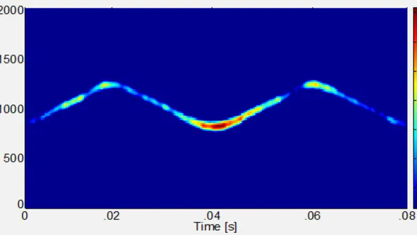
Testing was performed for a triangular modulated FMCW waveform (parameters: sampling frequency=6KHz; carrier frequency=1.5KHz; modulation bandwidth=2400Hz; modulation period=.015sec). The waveform parameters were chosen for academic validation of signal processing techniques. Due to computer processing resources they were not meant to represent real-world values. The number of samples for each test was chosen to be 512, which seemed to be the optimum size for the desktop computer. Testing was performed at three different Signal-to-Noise (SNR) levels: 10dB, 0dB, and the lowest SNR at which the signal could be detected. The noise added was white Gaussian noise, which best reflects the thermal noise present in the IF section of an intercept receiver [PAC09]. Kaiser windowing was used, when windowing was applicable. 100 runs were performed for each test, for statistical purposes. The time-frequency analysis techniques used for each task were the Scalogram and the Reassigned Scalogram.

After each particular run of each test, metrics were extracted from the time-frequency representation. The different metrics extracted were as follows:

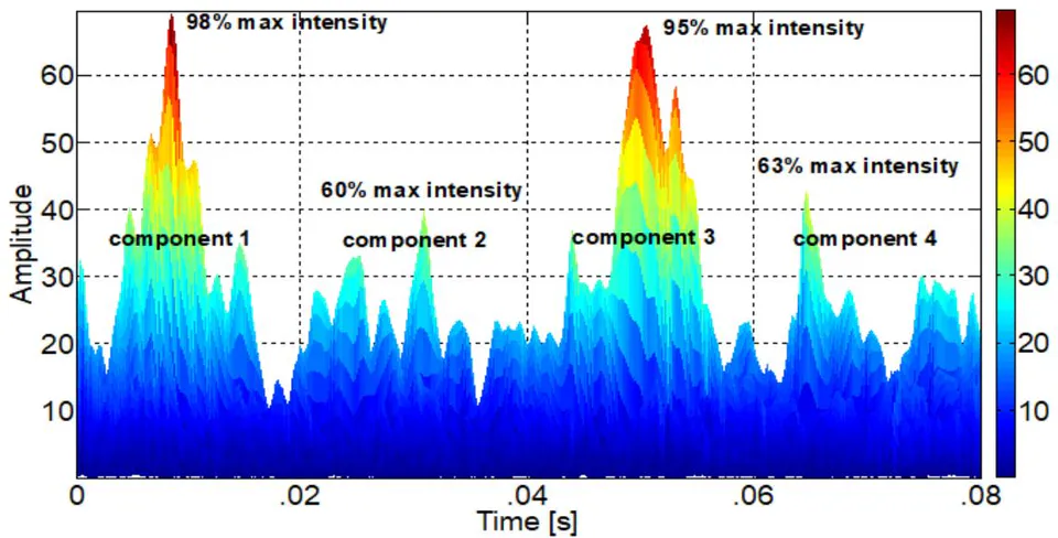
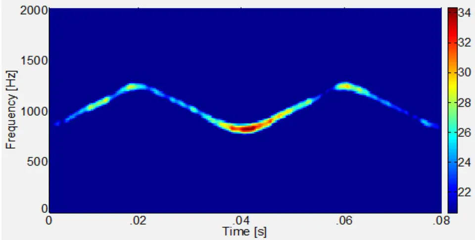
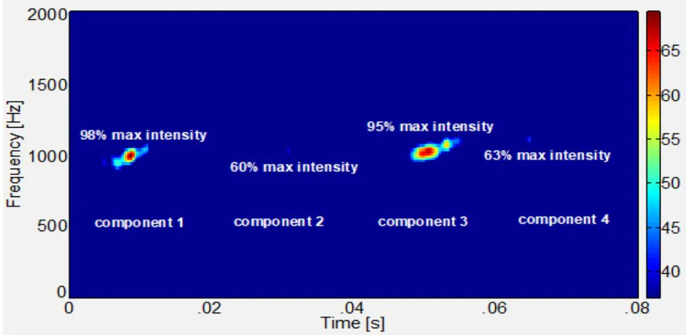
1. Percent detection: Percent of time signal was detected - signal was declared a detection if any portion of each of the signal components (4 chirp components for triangular modulated FMCW) exceeded a set detection threshold (a certain percentage of the maximum intensity of the time-frequency representation).

Detection threshold percentages were determined based on visual detections of low SNR signals (lowest SNR at which the signal could be visually detected in the time-frequency representation) (see Figure 1).

(Note - using this methodology, the detection threshold percentages were determined to be $50\mathrm{\%}$ for the Scalogram, and $50\mathrm{\%}$ for the Reassigned Scalogram. These values were automatically set for the plots in Figure 9 of the Results Section in this paper). Figure 1: Example plot for detection threshold percentage determination. This plot is an amplitude vs. time (x-z view) of a time-frequency analysis technique of a triangular modulated FMCW signal $(\mathrm{SNR}=-3\mathrm{dB})$. For visually detected low SNR plots (like this one), the percent of max intensity for the peak z-value of each of the signal components (the 2 legs for each of the 2 triangles of the triangular modulated FMCW) was noted (here $98\mathrm{\%}$, $60\mathrm{\%}$, $95\mathrm{\%}$, $63\mathrm{\%}$ ), and the lowest of these 4 values was recorded (here $60\mathrm{\%}$ ). This process was then repeated 25 times, and the average of the lowest values was calculated, and assigned as the detection threshold percentage for this time-frequency analysis technique For percent detection determination, these detection threshold values were included in the time-frequency plot algorithms so that the detection thresholds could be applied automatically during the plotting process. From the percent detection plot, the signal was declared a detection if any portion of each of the signal components was visible (see Figure 2).

Figure 2: Example plot for determination of percent detection (time-frequency). This plot is a frequency vs. time (x-y view) of a time-frequency analysis technique of a triangular modulated FMCW signal ( $SNR=10dB$ ) with detection threshold value automatically set to $60\mathrm{\%}$. From this plot, the signal was declared a (visual) detection because at least a portion of each of the 4 signal components (the 2 legs for each of the 2 triangles of the triangular modulated FMCW) was visible

1. Lowest detectable SNR: The lowest SNR level at which at least a portion of each of the signal components exceeded the set detection threshold listed in the percent detection section above.

For lowest detectable SNR determination, the detection threshold value was included in the time-frequency plot algorithms so that the detection threshold could be applied automatically during the plotting process. From the lowest detectable SNR plot, the signal was declared a detection if any portion of each of the signal components was visible. The lowest SNR level for which the signal was declared a detection is the lowest detectable SNR (see Figure 3).

Figure 3: Example plot for determining lowest detectable SNR. This plot is an frequency vs. time (x-y view) of a time-frequency analysis technique of a triangular modulated FMCW signal ( $SNR=-3dB$ ) with detection threshold value automatically set to $60\mathrm{\%}$. From this plot, the signal was declared a (visual) detection because at least a portion of each of the 4 signal components (the 2 legs for each of the 2 triangles of the triangular modulated FMCW) was visible. Note that the signal portion for the $60\mathrm{\%}$ max intensity (just above the 'x' in 'max') is barely visible, because the detection threshold for the time-frequency analysis technique is $60\mathrm{\%}$. For this case, any lower SNR would have been a non-detect. Compare to

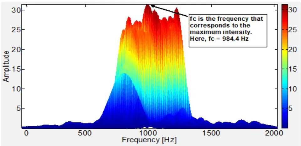
1. Carrier frequency: The frequency corresponding to the maximum intensity of the time-frequency representation (see Figure 4).

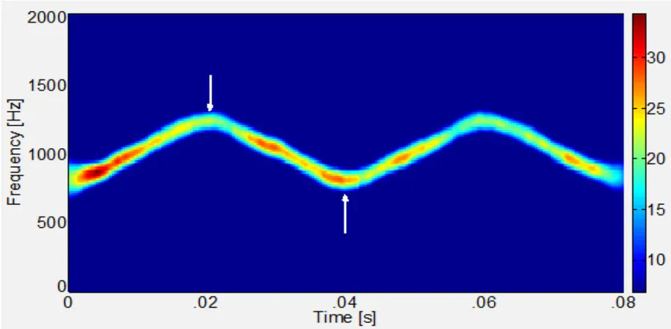
1. Modulation bandwidth (modBW): Distance from highest frequency value of signal (at a manual measurement threshold of $20\mathrm{\%}$ maximum intensity) to lowest frequency value of signal (at same threshold) in Y-direction (frequency).

The manual measurement threshold of $20\mathrm{\%}$ maximum intensity was determined based on manual measurement of the modulation bandwidth of the signal in the time-frequency representation. This was accomplished for 25 test runs for each time-frequency analysis technique, for each waveform. During each manual measurement, the max intensity of the high and low measuring points was recorded. The average of the max intensity values for these test runs, for each of the time-frequency analysis techniques, for each waveform, was $20\mathrm{\%}$. This was adopted as the manual measurement threshold value, and is representative of what is obtained when performing manual measurements. This manual measurment threshold of $20\mathrm{\%}$ maximum intensity was also adapted for determining the modulation period and the time-frequency localization (both are described below).

For modulation bandwidth determination, the manual measurement threshold of $20\mathrm{\%}$ maximum intensity was included in the time-frequency plot algorithms so that the threshold could be applied automatically during the plotting process. From the modulation bandwidth plot, the modulation bandwidth was manually measured (see Figure 5).

Figure 5: Example plot for modulation bandwidth determination. This plot is a time vs. frequency (x-y view) of a time-frequency analysis technique of a triangular modulated FMCW signal (SNR=10dB) with the manual measurement threshold of $20\mathrm{\%}$ maximum intensity automatically set. From this modulation bandwidth plot, the modulation bandwidth was measured manually from the highest frequency value of the signal (top white arrow) to the lowest frequency value of the signal (bottom white arrow) in the y-direction (frequency)

1. Modulation period (modPer): Distance from highest frequency value of signal (at a manual measurement threshold of $20\mathrm{\%}$ maximum intensity) to lowest frequency value of signal (at same threshold) in X-direction (time).

For modulation period determination, the manual measurement threshold of $20\mathrm{\%}$ maximum intensity was included in the time-frequency plot algorithms so that the threshold could be applied automatically during the plotting process. From the modulation period plot, the modulation bandwidth was manually measured (see Figure 6).

Figure 6: Example plot for modulation period determination. This plot is a time vs. frequency (x-y view) of a time-frequency analysis technique of a triangular modulated FMCW signal (SNR=10dB), with the manual measurement threshold of $20\mathrm{\%}$ maximum intensity automatically set. From this modulation period plot, the modulation period was measured manually from the highest frequency value of the signal (top white arrow) to the lowest frequency value of the signal (bottom white arrow) in the x-direction (time)

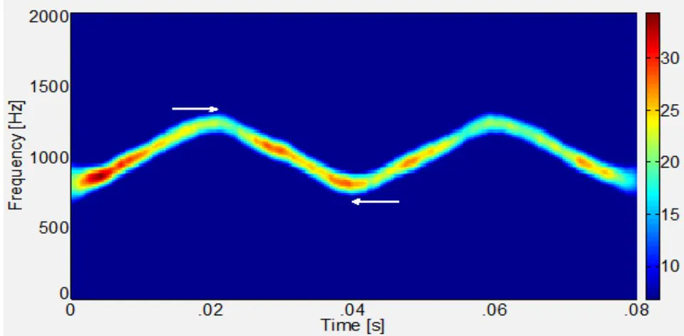
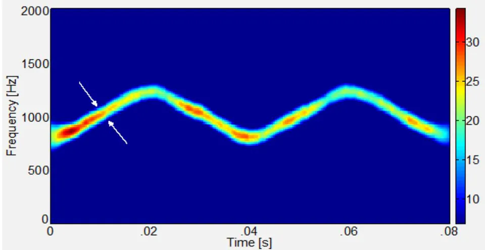
1. Time-frequency localization: Measure of the thickness of a signal component (at the manual measurement threshold of $20\mathrm{\%}$ maximum intensity) on each side of the component) – converted to $\mathrm{\%}$ of entire X-Axis, and $\mathrm{\%}$ of entire Y-Axis.

For time-frequency localization determination, the manual measurement threshold of $20\mathrm{\%}$ maximum intensity was included in the time-frequency plot algorithms so that the threshold could be applied automatically during the plotting process. From the time-frequency localization plot, the time-frequency localization was manually measured (see Figure 7).

Figure 7: Example plot for time-frequency localization determination. Time-frequency analysis technique of a triangular modulated FMCW signal (SNR=10dB) with the manual measurement threshold of $20\mathrm{\%}$ maximum intensity automatically set. From this time-frequency localization plot, the time-frequency localization was measured manually from the left side of the signal (left white arrow) to the right side of the signal (right white arrow) in both the x-direction (time) and the y-direction (frequency). Measurements were made at the center of each of the 4 'legs', and the average values were determined. Average time and frequency 'thickness' values were then converted to:% of entire x-axis and% of entire y-axis

7) Chirp rate: (modulation bandwidth)/(modulation period)

The data from all 100 runs for each test was used to produce the actual, error, and percent error for each of these metrics listed above.

The metrics from the Scalogram were then compared to the metrics from the Reassigned Scalogram. By and large, the Reassigned Scalogram outperformed the Scalogram, as will be shown in the results section.

VII. RESULTS

Table 1 presents the overall testmetrics for the two time-frequency analysis techniques used in this testing (Scalogram versus Reassigned Scalogram).

Parameters	Scalogram	Reassigned Scalogram
Carrier Frequency	9.09%	3.45%
Modulation Bandwidth	9.31%	2.88%
Modulation Period	0.61%	0.52%
Chirp Rate	9.57%	5.71%
Percent Detection	65.30%	72.10%
Lowest Detectable snr	-2.56db	-3.07db
Time-Frequency Localization-X	3.83%	2.14%
Time-Frequency Localization-Y	3.46%	1.28%

From Table 1, the Reassigned Scalogram outperformed the Scalogram in every metrics category. Note- using this methodology, the detection threshold percentages were determined to be $50\mathrm{\%}$ for the Scalogram, and $50\mathrm{\%}$ for the Reassigned Scalogram.

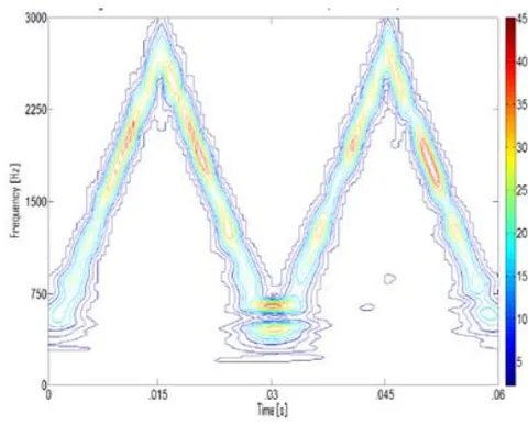
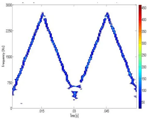
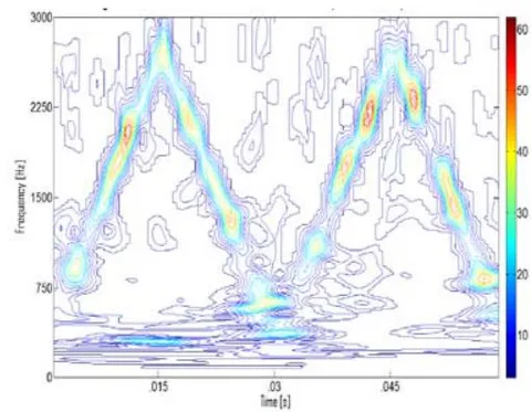
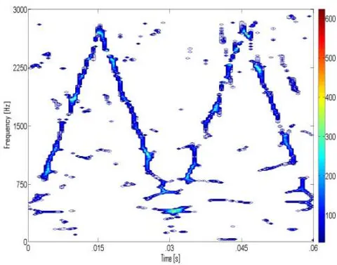
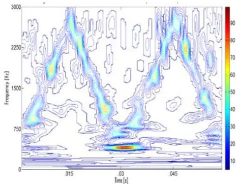
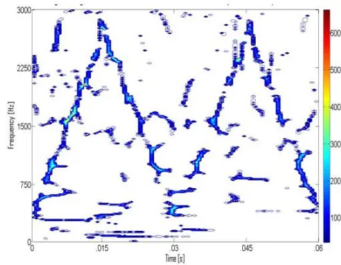
Figure 9 shows comparative plots of the Scalogram (left) vs. the Reassigned Scalogram (right) (triangular modulated FMCW signal) at SNRs of 10dB (top), 0dB (middle), and -3dB (bottom).

Figure 2, which is the same plot, except that it has an SNR level equal to 10dB

VIII. DISCUSSION

This section will elaborate on the results from the previous section.

From Table 1, the Reassigned Scalogram outperformed the Scalogram in every category. For the Scalogram, the poorer signal localization ('thicker' signal), when compared with the Reassigned Scalogram's 'squeezing' quality (see Figure 9), can account for the Scalogram being outperformed by the Reassigned Scalogram in the areas of: average percent error of modulation bandwidth, modulation period, chirp rate (=modBW/modPer)), time-frequency localization (x and y-direction), lowest detectable SNR, carrier frequency, and percent detection. Note that average percent detection and lowest detectable SNR are both based on visual detections in the time-frequency representation. Figure 9 shows that the signals in the Reassigned Scalogram plots are more readable than those in the Scalogram plots, which accounts for the Reassigned Scalogram's better average percent detection and lowest detectable SNR. The Scalogram might be used in a scenario with a 'quick and dirty' check to see if a signal is present, without accurate extraction of its parameters. The Reassigned Scalogram might be used in a scenario where you need accurate parameters, in a low SNR environment, in a quick time frame.

IX. CONCLUSIONS

Digital intercept receivers, whose main job is to detect and extract parameters from low probability of intercept radar signals, are currently moving away from Fourier-based analysis and towards classical time-frequency analysis techniques, such as the Scalogram, and Reassigned Scalogram, for the purpose of analyzing low probability of intercept radar signals. Based on the research performed for this paperit was shown that the Reassigned Scalogram by-and-large outperformed the Scalogram for analyzing these low probability of intercept radar signals - for reasons brought out in the discussion section above. More accurate characterization metrics could well translate into saved equipment and lives.

Future plans include analysis of additional low probability of intercept radar waveforms, using additional time-frequency analysis and reassignment method techniques.