I. INTRODUCTION

Hydrodynamic oscillation generators [1, 2] produce pressure waves when a fluid flows through channels of specific shapes and dimensions. These generators have no movable elements, which provides their reliability and long service life. Such devices can be used to disperse gas in liquid in many fields of chemical technologies [3], in systems for the biological purification of waste water and the chlorination and ozonization of drinking water, etc [2]. Generators of this type for medical purposes work like hydromassages [4]. Auspicious is the use such devices in oil production [5] to intensify oil production processes and enhance oil recovery. The results of wave technology processing of more than 1000 oil wells showed that the oil well productivity increased by an average of $30-40\mathrm{\%}$, and the oil recovery increased by $5-10\mathrm{\%}$.

It is necessary to develop methods for mathematical modeling to improve the performances of hydrodynamic generators. This method was presented in [6]. The system of continuity equation and Reynolds-averaged Navier-Stokes equations [7] with the "standard" $k$ -ε turbulence model [8, 9] and the full cavitation model [10] was solved. The amplitude-frequency characteristics of the oscillations were calculated. The calculated positions of the amplitude maxima agreed with the available experimental data.

However, the experience of using the model [6] showed that for some values of the operating parameters of the generators, instabilities of the calculation procedure arose, leading to the appearance of the negative pressure in the channel, which increased infinitely in absolute value. In addition, for those cases when these instabilities did not arise, the calculated pressure distributions along the channel wall differed markedly from the experimental values. It was suggested that these problems are related to the flow swirl, which is not considered in the "standard" $k$ -ε turbulence model [8, 9]. There are several experimental works that have shown that the swirl of the flow can lead to the weakening of turbulent pulsations.

In particular, Murakami and Kikuyama [12] studied the turbulent flow of water in a rotating tube. The water was supplied into a long fixed pipe with a diameter of D = 32 mm and a length of 60D, forming a steady turbulent longitudinal velocity profile. The unswirled flow entered the rotating pipe and was involved in the rotation due to friction against the walls. The rotating tube had segments of various lengths: 30D, 50D, 70D, 120D, 140D and 160D. Between these segments there were receivers of total pressure, which could move along the radius. The velocity profile was determined from the value of the dynamic pressure. The liquid then entered a fixed outlet pipe 200D long. The measurements showed that when moving along a rotating pipe, the profile of the axial velocity component changed and transformed from a steady turbulent to a parabolic one, which is typical for a laminar flow.

A.

I. Borisenko, O. N. Kostikov, and V.

I. Chumachenko [13] used a hot-wire anemometer to measure the intensity of turbulent pulsations in a rotating pipe with a diameter of $\mathrm{D}=52\mathrm{mm}$, through which an airflow passed. It was found that the intensity of pulsations decreases in the rotating channel. This process began at the wall, and as it moved away from the inlet, it reached the central region of the pipe. Thereby, under conditions typical of [12] and [13], the swirl led to flow laminarization. This must be taken into account in the mathematical model.

A correction to the $k$ - $\epsilon$ turbulence model for the flow swirl was proposed in [11]. The accounting for this amendment it made possible to achieve agreement between the calculated and experimental data on the pressure distribution along the channel wall of the hydrodynamic generator and to calculate amplitude-frequency characteristics. However, even with this correction, the instabilities of the calculation procedure as mentioned earlier arose in a number of cases. To overcome them, this paper proposes another form of correction for flow swirl.

II. MATHEMATICAL MODEL

The system of continuity equation (1) and Reynolds-averaged Navier-Stokes equations (2), (3), (4) for an axisymmetric flow [7] and the two-equation (5), (6) turbulence model [8, 9] was solved:

Here

Turbulent viscosity ${\mathbf{\Psi }}_{\mathrm{t}}$ was defined as

Two forms of corrections $f_{\mu }$ to turbulent viscosity, taking into account the flow swirl, were studied: quadratic (8) and linear (9):

Here $u$, $\nu$, and $w$ are the axial, radial, and tangential velocity components, $\rho$ is the fluid density, $k$ is the turbulence kinetic energy, and $\epsilon$ is the turbulence energy dissipation rate. In the absence of a swirl ( $w=0$ ), the presented turbulence model with each of the corrections (8) and (9) goes into the standard one [8].

The cavitation was taken into account using the equation of transfer of the vapor mass fraction [10]

Here, $f_{\mathrm{v}}$ is the mass fraction of vapor, ${\rho }_l$ is the density of the liquid, ${\rho }_{\mathrm{v}}=p_{\mathrm{sat}}{M}_{\mathrm{v}}/(RT)$ is the density of saturated vapor, $p_{\mathrm{sat}}$ is the pressure of saturated vapor of the liquid at temperature $T$, $M_{\mathrm{v}}$ is the molar mass of vapor, $p_{\mathrm{v}}=p_{\mathrm{sat}}+p_{\mathrm{turb}}/2$ is the phase-change threshold pressure, $p_{\mathrm{turb}}=0.39\rho k$ is the turbulent pressure fluctuations, $R_{\mathrm{ce}}$ is the rate of evaporation of the liquid (at ) or steam condensation (at ), $\sigma$ is the surface tension.

The system of equations (1) - (10) was solved by the pressure correction method [14] using the SIMPLE algorithm. In this method, instead of the continuity equation, the equation derived from it for corrections to pressure $p^{\prime }$ is solved. As the steady state solution is reached in the cycle of pressure iterations, the corrections $p^{\prime }$ approach zero.

Near the channel walls, in a laminar sublayer the near-wall functions proposed in [9] were used instead of Eq. (6).

In the calculation scheme of the generator (Fig. 1), the segments $AB$ and $EF$ are the face walls, $BE$ is the cylindrical wall of the channel, $FG$ is the cylindrical wall of the operation chamber, and $GH$ is the output cross-section. The supply orifices were placed in segment $CD$. The cross-section $I-I$ was set through the axes of symmetry of these orifices.

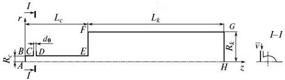
As boundary conditions on solid walls $AB$, $BC$, $DE$, $EF$, and $FG$ (Fig. 1), the no-slip conditions were set: $u=\upsilon =w=0$, $p^{\prime }=0$, $\partial p/\partial n=0$, $k=0$, $\partial \epsilon /\partial n=0$, $f_{\upsilon }=0$. where $n$ is the coordinate along the normal to the wall.

On the axis of symmetry $AH$: $\partial u/\partial r=0$, $\upsilon =w=0$, $\partial p^{\prime }/\partial r=0$, $\partial p/\partial r=0$, $\partial k/\partial r=0$, $\partial \epsilon /\partial r=0$, $\partial f_{\mathrm{U}}/\partial r=0$.

In the region of fluid inlet $CD$: $u=0$, $\upsilon ={\upsilon }_0$, $w=w_0$, $k=k_0$. $\epsilon ={\epsilon }_0$, $f_0=0$. Here are ${\upsilon }_0=Q/(2\pi R_c{d}_0)$, $w_0=4Q/(\pi d_0^2{n}_0)$, $k_0=(k_{in}{\upsilon }_0{)}^2/2$, ${\epsilon }_0=C_{\mu }{k}_0\sqrt{k_0}/(0.1d_0)$, $Q$ is the volumetric flow rate of the liquid, $n_0$ is the number of supply orifices. In this work it was taken $n_0=2$, $k_{\mathrm{in}}=0.05$.

At the output of $GH$: $p=p_{\mathrm{out}}$, and "soft" boundary conditions $\partial F/\partial z=0$, where $F$ is one of the variables: $u,v,w,p^{\prime },k,\epsilon$, and $f_0$.

III. OBJECT OF INVESTIGATION

An especial test generator (Fig. 2,a) was developed [16] to verify the mathematical model.

This generator made it possible to obtain the pressure distribution along the channel wall in order to compare calculated and experimental data.

The generator was of a cylindrical channel with a flaring part (operation chamber). The working fluid (tap water) was fed through two tangential orifices ensuring swirl of the flow. Six orifices in planes $xz$ and $yz$ have been made on a channel wall for static pressure measurement. Using of tubes the orifices were connected to manometers.

Tap water was chosen due to its availability. These generators can also operate on other liquids, particularly mineral oil and special drilling fluids.

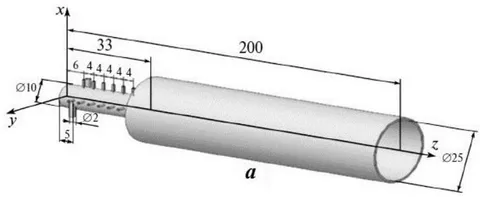
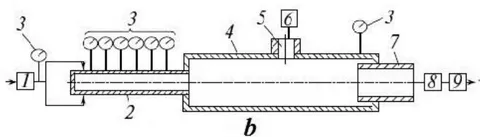
The experimental results of the study of this test generator were given in [16]. Experiments were performed on the facility, the scheme of which is presented in Fig. 2,b. The tap water was fed into the input of pump 1 and directed into the generator 2 under the pressure $p_{\mathrm{in}}$. The water pressure was measured by manometers 3 of the accuracy class 1. After the generator, the water entered operation chamber 4. The piezoelectric pressure sensor 5 of type 701A produced by Kistler was mounted to measure the pressure pulsations. The oscilloscope LeCroy Wave Surfer^f MXs-B 6 was used to record and proceed the spectra. The used water went to the drain through throttle 7, flowmeter 8, and adjusting ventil 9. The required pressure $p_{\mathrm{out}}$ in the chamber was set using ventil 9.

IV. RESULTS AND DISCUSSIONS

The results presented below were obtained at the value of absolute pressure of water $p_{\mathrm{in}}=5.1$ MPa at the generator input and $p_{\mathrm{out}}=0.24$ MPa at the generator output. The flow rate was equal to $Q=23.3{\mathrm{dm}}^3/\min$. The Reynolds number computed by the averaged velocity in the channel was $\mathrm{Re}\approx 50000$. These parameters corresponded to values typical for generators used in chemical technologies.

a) Time dependences of the pressure

The calculated dependences of pressure $p$ on time $t$ on the axis of symmetry $(r=0\mathrm{mm})$ in the cross-section of the supply orifices $(z=5\mathrm{mm})$ are shown in Fig. 3.

Figure 3: The time dependences of the pressure at the axis of symmetry at the plane of input orifices ( $r=0\mathrm{mm}$, $z=5\mathrm{mm}$ ): (a) without correction for the swirl ( $f_{\mu }=1$ ), (b) with a quadratic correction $f_{\mu }$ according to (8), (c) with a linear correction $f_{\mu }$ according to (9).

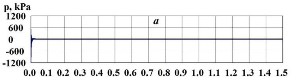
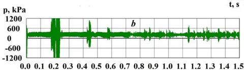
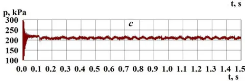
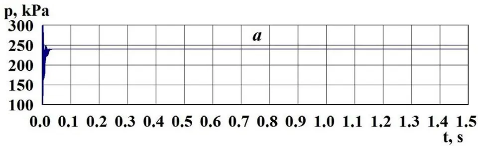
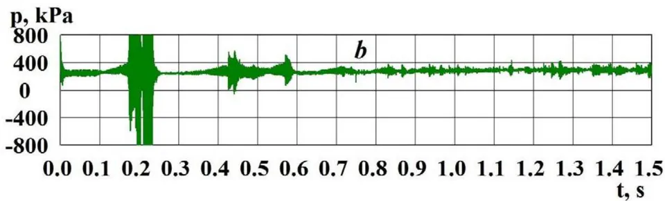
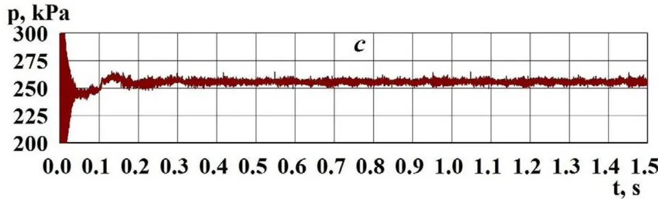
The calculation without correction for the swirl, $f_{\mu }=1$ (Fig. 3,a), led to the damping of pressure fluctuations with time. In contrast, in experiments [15, 16] these fluctuations existed constantly. The calculations with a quadratic correction for swirl according to expression (8) (Fig. 3,b) gave undamped oscillations in time. However, at some time intervals, instabilities of the calculation procedure were observed with a sharp increase in pressure in absolute value, which disappeared as the calculation continued. This significantly increased the calculation time required to achieve a steady state of oscillations. In addition, non-physical negative pressure values appeared at some channel points. The calculations with a linear correction for the swirl according to expression (9) (Fig. 3,c) gave stable fluctuations in time. In this case, there were no negative pressures.

Similar calculated data at the location of the pressure sensor in the experiments [15, 16]( $r=14\mathrm{mm},z=100\mathrm{mm}$ ) are shown in Fig. 4.

Figure 4: The time dependences of the pressure at the location of the pressure sensor ( $r=14\mathrm{mm}$, $z=100\mathrm{mm}$ ): (a) without correction for the swirl ( $f_{\mu }=1$ ), (b) with a quadratic correction $f_{\mu }$ according (8), (c) with a linear correction $f_{\mu }$ according (9).

b) Amplitude-frequency characteristics of the oscillations

By Fourier transformations of the data presented in Fig.4,b and 4,c, for time intervals of steady oscillations $t=0.6$... 1.5 s, the calculated amplitude-frequency characteristics of the oscillations were obtained (Fig. 5,a and 5,b). The corresponding experimental frequency response according to [15] is shown in Fig. 5, c.

A, kPa A, kPa

A, mV

Figure 5: The amplitude-frequency characteristics of the oscillations at the location of the pressure sensor ( $r=14\mathrm{mm}$, $z=100\mathrm{mm}$ ): (a) calculations with a quadratic correction $f_{\mu }$ according to expression (8), (b) with a linear correction $f_{\mu }$ according to expression (9), (c) experiment [15].

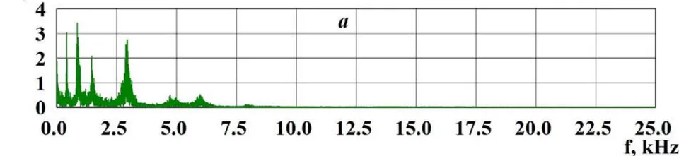
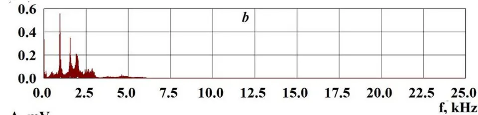
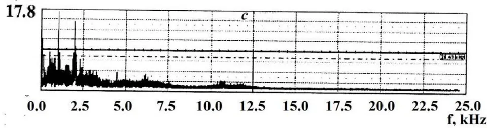
The experimental values of the amplitudes in Fig. 5, $c$ are presented in units of the oscilloscope scale (millivolts). The experimental frequency characteristic exhibits two principal maxima at frequencies $f=1.04\mathrm{kHz}$ and $f=1.98\mathrm{kHz}$. The calculated frequency characteristic with a quadratic correction according to expression (8) yielded four maxima at $f=0.42$, 0.83, 1.48, and $2.90\mathrm{kHz}$. The calculation with a linear correction using expression (9) gave the values of three principal maxima corresponding to the frequencies $f=0.94$, 1.55, and $1.98\mathrm{kHz}$.

c) The pressure distribution along a wall of the channel

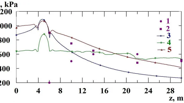
Experimental pressure distributions [16] along the wall of the generator channel ( $r=5\mathrm{mm}$ ) in a plane parallel to the axes of the supply orifices are shown in Fig. 6, points 1, and in the plane perpendicular to these axes in Fig. 6, points 2. It can be seen that deviations from axisymmetry manifest themselves up to distances $z=10\dots 12\mathrm{mm}$ from the left end wall of the channel.

Figure 6: The distribution of the time-averaged pressure along the wall of the generator channel: points (1) experiment in a plane $xz$ parallel to the axes of the supply orifices, points (2) experiment in a plane $yz$ perpendicular to the axes of the supply orifices, line (3) calculation without correction for the swirl ( $f_{\mu }=1$ ), line (4) calculation with quadratic correction $f_{\mu }$ according to expression (8), line (5) calculation with a linear correction $f_{\mu }$ according to expression (9)

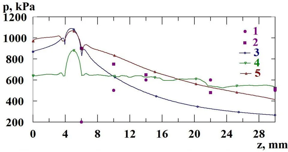
The calculations without considering the correction for the flow swirl (Fig. 6, line 3) showed a noticeable deviation from the experimental values. The calculated data obtained in the axisymmetric approximation with a quadratic correction $f_{\mu }$ (Fig. 6, line 4) according to expression (8) are between the experimental points, and with a linear correction $f_{\mu }$ (Fig. 6, line 5) according to expression (9) deviate slightly from experimental points.

V. CONCLUSIONS

1. In conditions, which are typical for hydrodynamic generators, the swirl of a stream leads to laminarization of the current. It occurs owing to the stabilising influence of a field of centrifugal forces. Besides, because of centrifugal effects the liquid is rejected on stream periphery where there is a damping of turbulent pulsations of speed due to a friction about a wall.

2. A comparison of two forms of corrections for the flow swirl in the $k$ - $\epsilon$ -model of turbulence is carried out. The accounting for these corrections it made possible to achieve consistency between the calculated and experimental data on the pressure distribution along the channel wall of the hydrodynamic generator and it made

• possible to calculate the amplitude-frequency characteristics of oscillations. If there is no swirl, both models shown are automatically converted to the standard $k$ - $\epsilon$ -model of turbulence.

1. The results obtained can be used in mathematical modeling of hydrodynamic oscillation generators for various purposes, particularly for chemical technologies, oil production and medicine.

ACKNOWLEDGMENTS

The author is grateful to the head of the Nonlinear Wave Mechanics and Technology Center of the RAS - the Branch of the Mechanical Engineering Institute of A. A. Blagonravov of the Russian Academy of Sciences, academician R. F. Ganiev, as well as the Center team for the help and useful work discussions. The author is especially grateful to O.

V. Shmyrkov for the provided experimental data.

The study was carried out using the computational resources of the Joint Supercomputer Center of the Russian Academy of Sciences (JSCC of RAS).