## I. INTRODUCTION Transfer Learning (Pan and Yang, 2009) is an important concept in machine learning research (Tan et al., 2018) that allows the domains, tasks, and distributions used in training and testing a network to be different from each other (Pan and Yang, 2010). Transfer learning is used to improve a learner from one domain by transferring information from a related domain (Weiss et al., 2016). The relatedness interacting domains cannot be over emphasized, as this could impact the relevance and appropriateness of the results However, the relatedness generated from such models. Transfer learning becomes a necessity when there is no large annotated dataset (a common case in medical image). This makes it imperative to use the knowledge about data learned from natural objects to learn patterns in medical images. However, the relatedness and sameness of the two (source and target) data distribution is a concern for this approach because the substantial difference between natural images and medical images may advice against such knowledge transfer (Tajbakhsh et al., 2016). Also, in relation to medical images which contain values that are proportional to the absorption characteristics of tissue with respect to a signal projected through the body (Petrou and Petrou, 2010), care should be taken to employ cross-domain transfer learning. Even though, transferring knowledge (learned features) from loosely related datasets such as ImageNet (Deng et al., 2009) to medical image in situations where there is insufficient ground-truth label may be promising, but it may introduce unintended biases which are undesirable in a clinical setting (Wang et al., 2018) As a result of the drawback of transfer learning especially in a sensitive domain like medicine, a better alternative is to train deep learning models exclusively of medical images. This is called training from scratch. Training a DL model from scratch is not without computational bottlenecks. This is why research in this area is limited because of insufficient labeled dataset (Tajbakhsh et al., 2016). However, advances in medical imaging technology and concern of deep learning research community on medical image analysis has led to the production of more radiological certified annotation on medical images. Notable among such is the National Institutes of Health (NIH) chest radiograph collection that consists of more than 100,000 chest radiographs with annotations (Wang et al., 2017). The Stanford University also released a very large dataset of chest radiographs with labels of pathology. This dataset contains over 200,000 open sourced chest x-rays (Irvin et al., 2019). Due to the availability of these dataset resources, one of the major reasons for cross-domain transfer learning has been eliminated. Data augmentation methods can be employed to extrapolate the available medical images to more than ten times the original quantity, so that more data could be used to learning medical image analysis models. Data argumentation techniques would also be such that would not remove relevant information from the medical images. Also, given that computational resources are available, then deep neural network models could be trained from scratch on medical images; hence this study. ## II. STATEMENT OF RESEARCH PROBLEM CXR are often characterized by variability in contrast intensity and texture, which are different from the content and structure of the images of natural object. Most of the existing deep models for medical image analysis are based on transfer learning that depends largely on the fine tuning of feature weights learned from natural image dataset. However, this cross-domain knowledge transfer is often not suitable for medical image analysis due to its inability to handle the variability in contrast intensity and texture that characterizes medical images. Again, in natural objects relative pixel intensity is used to convey information about a target object. That is, intensity variation and saturation are irrelevant when handling natural images. In contrast, medical images use exact pixel intensity values to convey information about abnormalities present in medical images. This intensity values are represented using the Hounsfield scale (Prince and Links, 2006). Also, location invariance does not affect the information content of natural images. In medical images on the other hand location is used to indicate pathological sites, because certain abnormalities are more likely to appear in certain part of a scan or x-ray. But the location of a dog or plate does not mean it is not a plate. Dimensionality reduction is a popular technique used to enhance the performance and efficiency of deep models, natural objects are scale invariant that is, and they retain their meaning irrespective of the scale. In medical images when the scales are change certain information-reach contents tend to lost. Deep learning models and architectures are developed using natural objects which still perform well with relative intensity, location and scale. Therefore, the outcome of medical image analysis from deep models that are trained using transfer learning mechanism are often not acceptable by the medical professionals and as such implemented CAD system from these deep models are rarely deployed for clinical practices. Therefore there is need to train medical image analysis models using medical image data; hence this study aims at developing a Deep Convolutional Neural Network model using domain-specific data for classification of abnormalities in chest x-rays. ## III. OBJECTIVES OF THE RESEARCH The specific objectives are to acquire and preprocess dataset of chest radiographs; formulate a deep network model for detecting abnormalities; evaluate the performance of the formulated model; and implement a prototype of the formulated model ## IV. CONCEPT OF TRANSFER LEARNING The concept of transfer learning was motivated by the fact that people can always apply previous knowledge to solve new problems faster (Torey and Shavlik, 2010) because repetition of common knowledge in the new task is abstracted away. It is a learning approach where knowledge from a domain is applied to solve a problem in another related domain. It is also referred to as domain adaptive learning (Kouw and Loog (2019). Transfer learning was inspired by the natural ability of human being to intelligently and intuitively apply knowledge from previous task to tackle new and previously unseen task. In ML applications, algorithms are developed to solve specific task such as classification, regression, or clustering problems. These algorithms often required labeled dataset for good generalization. It is expected that the training data and test data are in same feature space and from same marginal probability distribution, otherwise the model has to be reconstructed or modifications made to the algorithm. Transfer learning is the use of previously trained networks to mitigate the need for large dataset. There are two strategies for transfer learning practice (Litjens et al. 2017) 1. Using pre-trained network as feature extractor 2. Fine-tuning a pertained network on medical data Transfer learning performs better than training from scratch when a small data set like 1000 images are available (Menegola et al., 2016). Transfer learning is characterized by a domain $D = \{f_s, P(X)\}$ described by feature space fs and a marginal probability distribution $P(X)$ where each point in $X$ is an image vector, $x_i$ is the $i^{th}$ vector in a given learning sample $X$. For a given domain $D = \{f_s, P(X)\}$ a task in the domain consists of a label space ls and objective predictive function $f(\cdot)$ denoted by $f_o = \{Y, f(\cdot)\}$, with a training data $(x_i, y_i)$ where $x_i \in X$ is the input vector, $y_i \in Y$ is the label. For a new instance $x$, the objective function can be used to predict a new label. In Transfer Learning, two main domains stand out – the source domain denoted by $D_S$ and the target domain represented by $D_T$ with task $T_s$ and $TT$ respectively. Transfer learning thus aims at extracting the knowledge from one or more source tasks and apply the knowledge to a new (target) task (Pan and Yan, 2009). This is done by optimizing the learning of predictive function $f_T(\cdot)$ in $DT$ by utilizing the knowledge in $D_s$ and $T_S$ where $D_S \neq D_T$ or $T_S \neq T_T$ or $P_S(X) \neq P_T(X)$. Transfer learning is commonly used in deep learning applications, to access a pre-trained network and use it as a starting point to learn a new task and quickly transfer learned features to a new task using a smaller number of training images. This is because some low-level features are such as edges, shapes, corners and intensity are common to most domain. The concept is demonstrated in Figure 1, the figures show that the features learned from the source data (supposedly large dataset) are used to initiate learning in the target or new data (small dataset). Transfer learning can also come in three different flavors depending on the problem and resources at hand. There is minimum pre-processing procedure needed when transfer-learning techniques are used. However, no need for manual selection of Region of Interest (ROI). In addition, time-consuming weight training steps are removed because weights from source task are used for the target task. Deep learning resource hungry models can be done seamlessly small dataset and good performance. Transfer learning with its ability to recognize and apply knowledge and features learned in previous tasks to a novel task, is on the rise in recent years and has been applied in several data mining tasks, Zeiler and Fergus (2014). Transfer learning is often an attractive option when dealing with scarce data (Shin et al. 2016) for developing deep learning model where performance is based on seeing more data. The Image Net pre-trained model has been used to train several medical image analysis deep learning models with good and promising performance (Lakhani and Sundaram (2017)), Rajkoma et al. (2017), Shin et al. (2016), Baltrushchat et al. (2019). The practical implementation and deployment of these results are sparingly reported in healthcare institution. In medical domain, images consist of some specialty (view, features and modality) as pointed out earlier, thus transfer learning may be inappropriate for generalization. Training the neural networks from scratch would allow for learning more domain specific features corresponding to underlying pathological features rather than fine-tuning a network of natural images (Kumar, et al. (2017)). This is why transfer learning has proved to give outstanding performance when combined with handcraft domain features Bar et al. (2015). 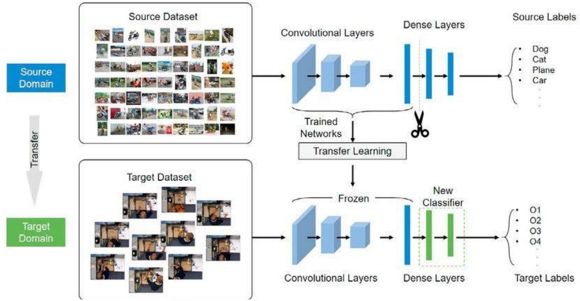 Figure 1: Transfer Learning Architecture (Tao, 2020) ## V. LIMITATION OF TRANSFER LEARNING IN MEDICAL DOMAIN (Tajbakhsh et al. (2016). Medical images are acquired by specialized instruments that significantly affect the result of computation. For instance, radiography images are produced by electromagnetic radiation projected by an X-ray generator to views the internal organs of the body. They are typically greyscale images. Also, there exist a measure of structural dissimilarity between medical images and natural objects, thus a seismic, hyperspectral or even medical imagery shows limited similarity with the images in ImageNet. Medical images consist of some inherent features and domain-specific specialties that could render transfer learning inappropriate. According to Kumar et al. (2017) training medical images from scratch for the purpose of analysis would allow for learning more specific features corresponding to underlying pathologies than transfer learning. Another important concern is that medical images are acquired from a number of clinical processes such as imaging of anatomy and physiology, interventional radiology and therapy. For instance, radiographic images characterized with salient features that reveals densities such as air, fat, muscle, bone, metals, and high contrast variations. In CT images soft tissues, rendered contours are common indications of importance. Also, to produce a quality medical image the orientation or view is of great importance as it contributes to the features used for its characterization. For instance, some clinical deviations are better diagnosed on a given view or orientation than the other. At a closer look, to get image correctly on SPECT, measurement at different angles/positions and projections are considered. For PET imaging the emission of photons and the angle between the positrons are important. MRI images on the other hand are commonly used on soft tissue image production, blood flow, cerebral diagnosis and cardiology; hence, they tend to pay attention to blood, water, and signal from the body. Medical image modality is an important aspect of image acquisition and interpretation process, because according to Clinicians, one of the most important filters that would enhance retrieval result significantly is the modality (de Herrera et al. 2013). Therefore, images of natural object (as in ImageNet) would not be appropriate for generalization in the medical domain because, the vulnerability of DNNs in medical imaging is crucial because the clinical application of deep learning needs extreme robustness for the eventual use in patients, compared to relatively trivial non-medical tasks, such as distinguishing cats or dogs (Yamashita et al., 2018). ## VI. DATA COLLECTION AND DESCRIPTION For this study, the CheXpert dataset was used. The CheXpert dataset is a compilation of radiographic studies that is online but domiciled in Stanford Hospital. It comprises of radiological reports from October, 2002 to July, 2017 on both in-patient and out-patients' cases. It was compiled by the Stanford University Machine Learning Group. The dataset contains 224,316 chest radiograph images of 65,240 patients. It consists of fourteen (14) radiological observations with consideration for uncertainty in radiograph interpretation. ### a) Dataset Preparation and Preprocessing To ease label matching to images, the uncertainty labels (-1.0) was converted to positive labels (1.0). This is to achieve a binary mapping of all labels similar with the $U$ -ones model of Irvin et al. (2019). In statistic this is called zero imputation strategy (Kolesov et al. 2014). The assumption here is that diseases that are not sure to be present in the CXR (uncertainty label) could be coded as present. On the other hand, label categories that are referred to as unmentioned (blanks cells) were coded as negative (0.0) or absent. This approach follows the principle in literature which is known as zero imputation strategies in statistics and similar to the multi-label classification method where missing examples are used as negative labels (Kolesov et al., 2014, Irvin et al., 2019). The conversion was carried out using the Keras Pandas version 0.24.1 data frame. As part of image pre-processing technique, all images were set to have the same aspect ratio and dimension.  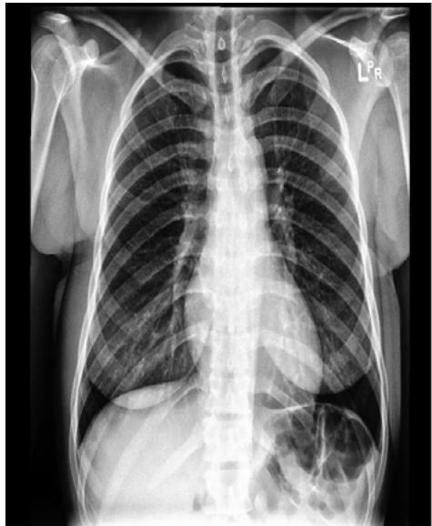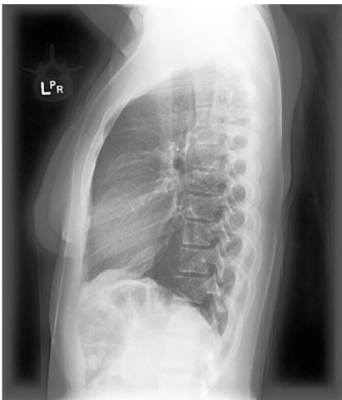A: Frontal View  B: Lateral View Figure 2: Views of CXR in CheXpert Dataset (Source: Irvin et al, 2019). Table 1: Sample of the CheXpert Observations showing 14 labels <table><tr><td>Pathology</td><td>Positive (%)</td><td>Uncertain (%)</td><td>Negative (%)</td></tr><tr><td>No Finding</td><td>16627 (8.86)</td><td>0 (0.0)</td><td>171014 (91.14)</td></tr><tr><td>Enlarged Cardiom.</td><td>9020 (4.81)</td><td>10148 (5.41)</td><td>168473 (89.78)</td></tr><tr><td>Cardiomegaly</td><td>23002 (12.26)</td><td>6597 (3.52)</td><td>158042 (84.23)</td></tr><tr><td>Lung Lesion</td><td>6856 (3.65)</td><td>1071 (0.57)</td><td>179714 (95.78)</td></tr><tr><td>Lung Opacity</td><td>92669 (49.39)</td><td>4341 (2.31)</td><td>90631 (48.3)</td></tr><tr><td>Edema</td><td>48905 (26.06)</td><td>11571 (6.17)</td><td>127165 (67.77)</td></tr><tr><td>Consolidation</td><td>12730 (6.78)</td><td>23976 (12.78)</td><td>150935 (80.44)</td></tr><tr><td>Pneumonia</td><td>4576 (2.44)</td><td>15658 (8.34)</td><td>167407 (89.22)</td></tr><tr><td>Atelectasis</td><td>29333 (15.63)</td><td>29377 (15.66)</td><td>128931 (68.71)</td></tr><tr><td>Pneumothorax</td><td>17313 (9.23)</td><td>2663 (1.42)</td><td>167665 (89.35)</td></tr><tr><td>Pleural Effusion</td><td>75696 (40.34)</td><td>9419 (5.02)</td><td>102526 (54.64)</td></tr><tr><td>Pleural Other</td><td>2441 (1.3)</td><td>1771 (0.94)</td><td>183429 (97.76)</td></tr><tr><td>Fracture</td><td>7270 (3.87)</td><td>484 (0.26)</td><td>179887 (95.87)</td></tr><tr><td>Support Devices</td><td>105831 (56.4)</td><td>898 (0.48)</td><td>80912 (43.12)</td></tr></table> Table 2: Summary of Model Parameters <table><tr><td></td><td>Initialized Value</td></tr><tr><td>Batch size</td><td>5</td></tr><tr><td>Initial Learning Rate</td><td>0.001</td></tr><tr><td>Epoch</td><td>10</td></tr><tr><td>Epsilon</td><td>1e-07</td></tr><tr><td>Kernel size</td><td>4 * 4</td></tr></table> ## VII. ANALYSIS OF RESULT FROM THE DEVELOPED MODEL The entire dataset was not used for the model training because of the unexpected computational complexity and overhead. Attempt on training the model in the entire training set produced a memory error. As a result, the training was carried out on the 234 images of the validation set with 0.1 used as test case. The network was trained over 10 epochs, this means that the model iterated over the train dataset 10 times. The model summary is represented graphically as model loss, model accuracy and the AUR ROC curve. Also, after model training Precision, recall, F- score and the accuracy was given as output. From Figure 3, the model accuracy showed that the accuracy increases rapidly in the first two epochs, indicating that the network is learning fast. Also, it showed that the model could probably be trained a little more as the trend for accuracy on both datasets is still rising for the last few epochs. Again, it is seen that the model has not yet over-learned the training dataset. From the Model loss curve as shown in Figure 4, loss was decreasing over time. This means that the model is really learning. The validation loss was high at the beginning of the learning process and decreases as epoch increases. The model would be better if the number of epoch increases. However considering the computational overhead, this study is limited to 10 epochs. From the model loss curve, there is evidence of unrepresentative training dataset. This happens when the data available during training is not enough to capture the model, in relation to the validation dataset. This was because sufficient data was not use for the model training. Increasing the training data would decrease the generalization error because the model becomes more general by virtue of being trained on more examples. The AUC ROC curves showed in comparison the probability of occurrence of all abnormalities on the testcase.  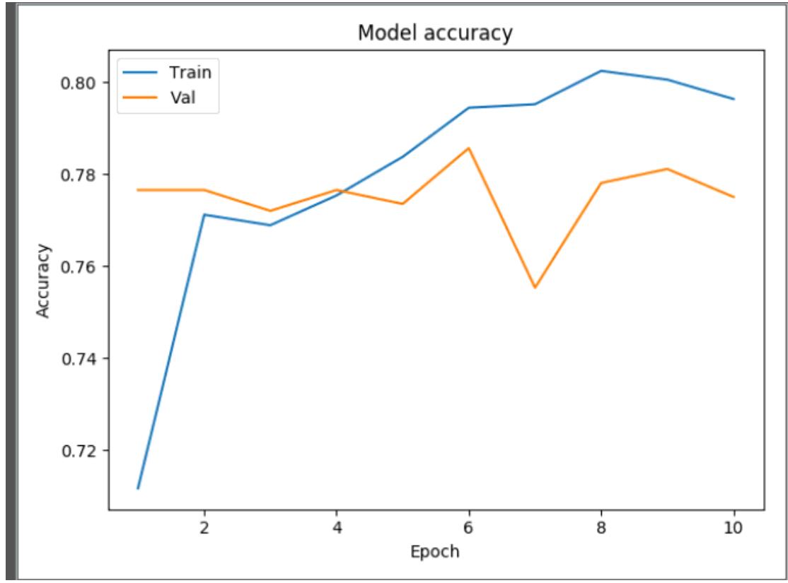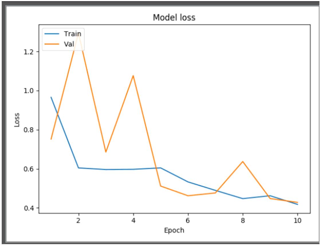Figure 3: Model Accuracy plot  Figure 4: Model Loss Plot 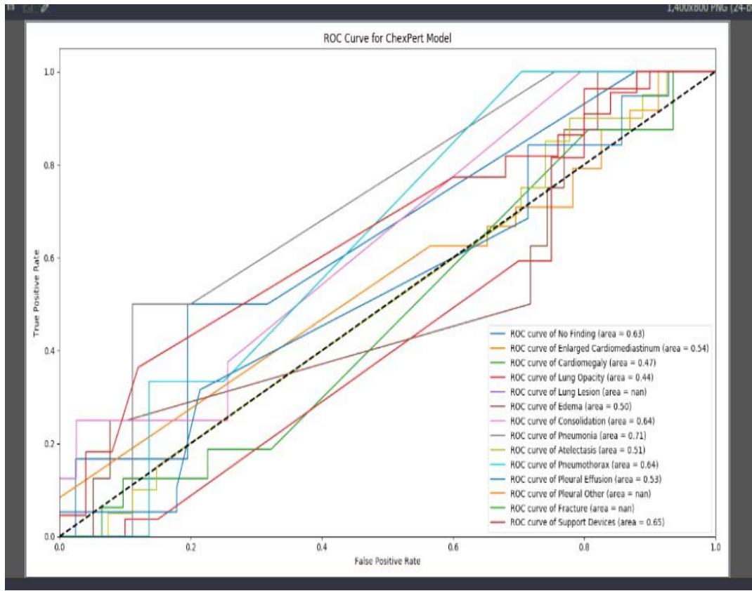 Figure 5: AUC ROC curve ## VIII. AUC ROC ANALYSIS OF RESULT The AUC ROC curve presented in Figure 5 was used to visualize all the performance metrics from a single image (a test image). The ROC curve was plotted for all the abnormalities present in the CXR of the CheXpert dataset. Table 3 captures the recorded probability values from the AUC ROC curve. From the AUC ROC curve, the developed model discriminated against some abnormality. Using the user-defined threshold value of 0.5, the threshold value was got from the average of the probability outcome of 0.57. Therefore, the developed model confidently detected the presence Atelestasis, Support devices, Pleural effusion, Pneumonia, A normal CXR (no finding), Pneumothorax, and Consolidation. This happened because the probability score was beyond the set threshold. However the model was detected the following abnormality as absence using the user defined threshold value of 0.5. That is, the probability outputs of Lung opacity and Cardiomegaly were less than 0.5. Table 3: Probability Output on the AUC ROC Curve <table><tr><td>Features (abnormality)</td><td>Output probabilities</td></tr><tr><td>No finding (normal)</td><td>0.63</td></tr><tr><td>Enlarged Cardio</td><td>0.54</td></tr><tr><td>Cardiomegaly</td><td>0.47</td></tr><tr><td>Lung opacity</td><td>0.44</td></tr><tr><td>Lung lesion</td><td>Nan</td></tr><tr><td>Edema</td><td>0.50</td></tr><tr><td>Consolidation</td><td>0.64</td></tr><tr><td>Pneumonia</td><td>0.71</td></tr><tr><td>Atelectasis</td><td>0.51</td></tr><tr><td>Pneumothorax</td><td>0.64</td></tr><tr><td>Pleural effusion</td><td>0.53</td></tr><tr><td>Pleural Other</td><td>Nan</td></tr><tr><td>Fracture</td><td>Nan</td></tr><tr><td>Support Devices</td><td>0.65</td></tr></table> The developed model was not able to detect lung lesion, pleural other and fracture therefore a NAN value was returned. The accuracy of the model was approximately 0.78. This means the model can predict the presence of an abnormality 78 times in a given 100 cases. Precision and recall had the same have value that is 0.78. ## IX. CONCLUSION This research has developed a model with medical images using Convolutional Neural Network. This is called training from the scratch because it does not involve the use of pre-trained weights. The developed model was based on the binary loss function because the problem was reduced to a binary multi-label problem where the model could detect the presence (1) or absence (0) of abnormalities under consideration. Fourteen (14) abnormalities associated with chest x-rays were examined in this study. The choice of model parameter was hampered by the limitation of computational resources. Hence, the only parameter that was tweaked was the batch size and image dimension. The two parameters were adjusted to optimally utilize the available computational resources. Image was down-sized to $250 \times 240$ and the batch size was changed often time but was pegged to 6 at the last computation stage. The number of network layer was only five, namely, the input layer, convolution layer, pooling layer and the fully connected layer. The model favorably predicted some abnormalities such as pneumonia, consolidation, pleural effusion, normal chest x-rays, pnuemothorax. On the other hand abnormalities such as lung opacity and cardiomegaly were not well predicted by the model. Model returned a null value for lung lesion, pleural other and fracture due the presence of uncertainty label. To handle label co-occurrence the model threshold was used to determine abnormalities that have likelihood of co-occurring in a chest x-ray. ## X. LIMITATION OF THE WORK AND FUTURE RESEARCH DIRECTION The research is however faced with a lot of issue on computational resource. Training model from scratch is highly computationally intensive. This was a serious limitation to getting the desired performance. Also a lot of parameter that was supposed to be tweaked was not done. The model has only four (4) Convolution layers which supposed to be deeper. Data augmentation was not carried out because the original training data of approximately 234,000 images were not utilized because of the processing capacity of the machine and the dimension of the input data. Care was taken not to downsize the image size more that necessary to avoid image degradation and loss of details from the chest x-ray. Transfer learning is a fast and quick technique for developing deep learning model, but on medical images it weight must be from domain similar to medicine. Also, more computational resources like High Performing Computers (HPC) so that massive data could be used.

Generating HTML Viewer...

References

23 Cites in Article
S Pan,Q Yang (2009). A Survey on Transfer Learning.
Weike Pan,Evan Xiang,Nathan Liu,Qiang Yang (2010). Transfer Learning in Collaborative Filtering for Sparsity Reduction.
Nima Tajbakhsh,Jae Shin,Suryakanth Gurudu,R Hurst,Christopher Kendall,Michael Gotway,Jianming Liang (2016). Convolutional Neural Networks for Medical Image Analysis: Full Training or Fine Tuning?.
Maria Petrou,Costas Petrou (2010). Image Processing: The Fundamentals.
B Wang,Y Yao,B Viswanath,H Zheng,B Zhao (2018). USENIX Security Symposium.
Xiaosong Wang,Yifan Peng,Le Lu,Zhiyong Lu,Mohammadhadi Bagheri,Ronald Summers (2017). ChestX-Ray8: Hospital-Scale Chest X-Ray Database and Benchmarks on Weakly-Supervised Classification and Localization of Common Thorax Diseases.
Jeremy Irvin,Pranav Rajpurkar,Michael Ko,Yifan Yu,Silviana Ciurea-Ilcus,Chris Chute,Henrik Marklund,Behzad Haghgoo,Robyn Ball,Katie Shpanskaya,Jayne Seekins,David Mong,Safwan Halabi,Jesse Sandberg,Ricky Jones,David Larson,Curtis Langlotz,Bhavik Patel,Matthew Lungren,Andrew Ng (2019). CheXpert: A Large Chest Radiograph Dataset with Uncertainty Labels and Expert Comparison.
J Prince,J Links (2006). Medical Imaging Signals and Systems.
L Torrey,J Shavlik (2010). Transfer Learning in Handbook of Research on Machine Learning Applications and Trends: Algorithms, Methods, and Techniques.
Wouter Kouw,Marco Loog (2019). A Review of Domain Adaptation without Target Labels.
A Menegola,M Fornaciali,R Pires,S Avila,E Valle (2016). Towards Automated Melanoma Screening: Exploring Transfer Learning Schemes.
Matthew Zeiler,Rob Fergus (2014). Visualizing and Understanding Convolutional Networks.
Paras Lakhani,Baskaran Sundaram (2017). Deep Learning at Chest Radiography: Automated Classification of Pulmonary Tuberculosis by Using Convolutional Neural Networks.
Alvin Rajkomar,Sneha Lingam,Andrew Taylor,Michael Blum,John Mongan (2017). High-Throughput Classification of Radiographs Using Deep Convolutional Neural Networks.
Hoo-Chang Shin,Holger Roth,Mingchen Gao,Le Lu,Ziyue Xu,Isabella Nogues,Jianhua Yao,Daniel Mollura,Ronald Summers (2016). Deep Convolutional Neural Networks for Computer-Aided Detection: CNN Architectures, Dataset Characteristics and Transfer Learning.
Ivo Baltruschat,Hannes Nickisch,Michael Grass,Tobias Knopp,Axel Saalbach (2019). Comparison of Deep Learning Approaches for Multi-Label Chest X-Ray Classification.
Sanjeev Kumar,Chetna Dabas,Sunila Godara (2017). Classification of Brain MRI Tumor Images: A Hybrid Approach.
A De Herrera,J Kalpathy-Cramer,D Demner-Fushman,S Antani,H Müller (2013). Overview of The Imageclef 2013 Medical Tasks.
Yaniv Bar,Idit Diamant,Lior Wolf,Sivan Lieberman,Eli Konen,Hayit Greenspan (2015). Chest pathology detection using deep learning with non-medical training.
Wenjin Tao,Md Al-Amin,Haodong Chen,Ming Leu,Zhaozheng Yin,Ruwen Qin (2020). Real-Time Assembly Operation Recognition with Fog Computing and Transfer Learning for Human-Centered Intelligent Manufacturing.
Chuen-Kai Shie,Chung-Hisang Chuang,Chun-Nan Chou,Meng-Hsi Wu,Edward Chang (2015). Transfer representation learning for medical image analysis.
Rikiya Yamashita,Mizuho Nishio,Richard Do,Kaori Togashi (2018). Convolutional neural networks: an overview and application in radiology.
No ethics committee approval was required for this article type.
Data Availability
Not applicable for this article.
How to Cite This Article
Joy Nkechinyere Olawuyi. 2026. \u201cDomain Specific Deep Neural Network Model for Classification of Abnormalities on Chest Radiographs\u201d. Global Journal of Computer Science and Technology - D: Neural & AI GJCST-D Volume 23 (GJCST Volume 23 Issue D1): .
Explore published articles in an immersive Augmented Reality environment. Our platform converts research papers into interactive 3D books, allowing readers to view and interact with content using AR and VR compatible devices.
Your published article is automatically converted into a realistic 3D book. Flip through pages and read research papers in a more engaging and interactive format.
This study collected, pre-processed dataset of chest radiographs, formulated a deep neural network model for detecting abnormalities. It also evaluated the performance of the formulated model and implemented a prototype of the formulated model. This was with the view to develop a deep neural network model to automatically classify abnormalities in chest radiographs. In order to achieve the overall purpose of this research, a large set of chest x-ray images were sourced for and collected from the CheXpert dataset, which is an online repository of annotated chest radiographs compiled by the Machine Learning Research group, Stanford University. The chest radiographs were preprocessed into a format that can be fed into a deep neural network. The preprocessing techniques used were standardization and normalization. The classification problem was formulated as a multi-label binary classification model, which used convolutional neural network architecture for making decision on whether an abnormality was present or not in the chest radiographs. The classification model was evaluated using specificity, sensitivity, and Area Under Curve (AUC) score as parameter.
Our website is actively being updated, and changes may occur frequently. Please clear your browser cache if needed. For feedback or error reporting, please email [email protected]
Thank you for connecting with us. We will respond to you shortly.