1. Introduction
1.1. Background of the study
The agriculture sector employs 80% of the population of Rwanda and contributes 33% of GDP growth. Agriculture is the backbone and a key component of Rwanda's fast-growing economy. In recent years, the sector has gained significant growth from 4.5% to 6% per annum and is gradually shifting from a subsistence model to a market-oriented model. According to research conducted by Habineza et al. [36], Postel et al. [69], and RAO [73], irrigation contributes to agricultural growth and reduces poverty directly by permitting intensification and diversification, leading to increased outputs and incomes, higher agricultural wage employment, and lower local food prices. Irrigation has contributed significantly to poverty alleviation, food security, and improving the quality of life for rural populations. In addition, according to the National Institute of Statistics of Rwanda [77], overall 4% of agricultural areas are irrigated in Season A, with no irrigation for crops in hillside and rangeland areas and 26% irrigation in marshlands. The highest irrigation rates were found in Huye District (19%) and Rusizi District (18%).
Although Rwanda has abundant water resources, they are not evenly distributed. Rainfall is high in the western part of the country and low in the east. Rainfall variability is critical for lands on hillsides where water cannot be retained, making farms in the eastern part of the country the most vulnerable. Regarding surface water bodies, eastern Rwanda has abundant rivers and lakes that can be harnessed for irrigation. For groundwater resources, the central and eastern parts of the country indicate good potential, especially for springs and borehole development [85]. Currently, the most commonly used method is flood irrigation in marshlands, though demonstration farms are being established in drought-prone eastern Rwanda to educate farmers on irrigation advantages. Where irrigation has been introduced, a doubling of yields is commonly achieved [85].
Drip irrigation figures prominently in proposed solutions to the water crisis and is promoted in national and international policy documents as a technology to use water more efficiently [73, 90]. Postel et al. [69] and RAO [73] report that drip irrigation has the potential to at least double crop yield per unit water in many applications, including vegetables, cotton, sugarcane, and orchard and vineyard crops. Research results from Indian institutes indicate typical water use reductions with drip irrigation of 30–60% and typical yield increases of 20–50% across cotton, sugarcane, grapes, tomatoes, and bananas, producing a doubling or tripling of water productivity [69]. Similarly, Van der Kooij et al. [90] note that shifting from conventional surface irrigation to drip irrigation in India increased overall water productivity by 42–255% for banana, cotton, sugarcane, and sweet potato [50]. Drip irrigation uses 30–50% less water than surface irrigation, reduces salinization and waterlogging, and achieves up to 95% irrigation efficiency [90].
1.2. Problem statement
Dry farming systems depend on precipitation, specifically green water stored directly in the soil and used via evapotranspiration. In water-scarce regions, green water resources make up 85% to 90% of precipitation, sustaining rain-fed agriculture. Due to a lack of water storage and large spatial and temporal variations in rainfall, most farmers cannot produce more than once per year, and frequent crop failures from dry spells and droughts result in food shortages. While development agencies have encouraged farmers to adopt treadle pumps, pitcher pot systems, micro-irrigation systems, and water harvesting techniques with mixed success, there is a tendency to over-emphasize the technology itself rather than the process by which it is identified, modified, and disseminated.
Currently, Rwanda is promoting horticultural crop farming through advanced irrigation technology adoption to increase export volumes on international markets. However, no specific study had been conducted in Rwanda to assess the performance of a drip irrigation system on carrot production. Consequently, this research analyzes weather parameters, soil physical and chemical properties (such as bulk density, porosity, and infiltration rate), and the uniformity coefficient and application uniformity of water under a drip irrigation system at the IPRC Gishari farm.
1.3. Objectives of the study
1.3.1. Overall objective
The overall objective of the study is the performance evaluation of the drip irrigation system on carrot production at the IPRC Gishari farm in Rwanda.
1.3.2. Specific objectives
- To determine the weather parameters of the experimental site.
- To determine the soil properties at the experimental site.
- To determine the water requirement, water deficit, and irrigation scheduling of carrot using CROPWAT 8.0.
- To assess the uniformity coefficient of water under the drip irrigation system.
- To assess the yield of carrot under drip irrigation in the experimental plots.
1.3.3. Research questions
- What are the weather characteristics of the IPRC Gishari farm?
- What are the soil physical and chemical properties at the IPRC Gishari farm?
- What are the crop water requirement, water deficit, and drip irrigation schedule of the carrot crop?
- What is the uniformity coefficient of water for the carrot crop under the drip irrigation system?
- What is the yield of carrot under the drip irrigation system in the experimental plots?
1.4. Scope and limitation of this research
This research evaluates the performance of drip irrigation on carrot production at the IPRC Gishari farm, examining the effects of weather parameters and soil properties. Crop water requirements and irrigation schedules are modeled using CROPWAT 8.0 software, while emitter uniformity coefficients, application uniformity, and carrot yields are determined experimentally from field plots.
1.5. Significance of the study
Understanding the causes of low horticultural crop productivity in the region requires assessing soil physical and chemical properties and their effects on crops under drip irrigation. Scaling up productivity and quality supports national goals of improving export earnings and meeting domestic consumption and processing demands. Furthermore, this study serves as reference material for researchers and helps policymakers and practitioners formulate strategies to optimize drip irrigation systems and soil management for smallholder farmers in Rwanda.
1.6. Thesis Outline
This study is organized into five main chapters. Section 1 provides the background, problem statement, objectives, and research questions. Section 2 reviews literature on weather parameters, soil physical and chemical properties, crop water requirements and scheduling via CROPWAT 8.0, water application uniformity, and carrot yield. Section 3 describes the study area, materials, field and laboratory methodologies, and statistical procedures. Section 4 presents the experimental results and discussions, and Section 5 provides the summary, conclusions, and recommendations.
2. Literature Review
2.1. Introduction
This section reviews existing literature regarding the influence of weather parameters on crop production, soil physical and chemical properties, crop water requirements and irrigation scheduling, emitter uniformity coefficients, and carrot yield under drip irrigation.
2.2. Weather Parameters on Carrot Production
Weather represents the combination of humidity, precipitation, wind, cloudiness, and atmospheric conditions at a specific time, whereas climate represents the long-term characteristic atmospheric conditions near the Earth's surface at a given location.
2.2.1. Rainfall
In Rwanda's Eastern Province, particularly around the Gishari farm plantation, rainfall is characterized by moderate to heavy rains from February to May and September to December, with drier periods from mid-December to mid-February and June to August [48]. Across eight rainfall stations at the Rwamagana plantation, annual rainfall ranged from a low of 850 mm in 2005 to a high of 1200 mm in 2006, and annual rainfall in Rwanda generally varies with altitude.
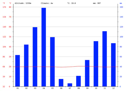
Huang et al. [41] demonstrated that sufficient rainfall in the second half of the growing season strongly influences crop yields. Rwamagana is classified as tropical savanna climate (Aw) under the Köppen-Geiger system, with an average annual temperature of 19.8 °C, mean annual rainfall of 907 mm, and an altitude of 1550 m (see Figure 1).
2.2.2. Minimum and Maximum Temperature
Carrots are a cool-weather crop requiring moderate temperatures for optimal development, whereas warmer temperatures are primarily tolerated early in the growing process [25, 79]. Sebaziga Ndakize [82] noted that Rwanda contains microclimatic zones with significant deviations from annual average temperatures, directly impacting crop development and productivity. Rahman et al. [72] utilized monthly mean, maximum, and minimum surface air temperature data to evaluate climatic variability.
Autovino, Rallo, and Provenzano [9] noted that ordinary linear regression:
captures temperature correlations, where represents the rate of change and represents monthly or seasonal temperature at time . Liyanage et al. [57] averaged daily maximum temperature, minimum temperature, and relative humidity on a weekly basis using Inverse Distance Weighting (IDW) interpolation. Sammis and Wu [80] and Liao, Zhang, and Bengtsson [55] showed that temperature variations significantly affect water consumption and crop yields under drip irrigation [27].
Nsengiyumva et al. [61] reported that maximum daytime temperatures typically occur between 3:00 PM and 7:00 PM, while minimum temperatures occur between 4:00 AM and 9:00 AM, depending on sky conditions, wind direction, and wind speed [59, 100]. High temperatures above 32 °C to 38 °C combined with low humidity can induce floral sterility and reduce fertilization in sensitive crops [83, 86].
2.2.3. Relative Humidity
Relative humidity is the ratio of the partial pressure of water vapor to the equilibrium vapor pressure of water at a given temperature [18]. It is higher in cool air than in warm air for a constant vapor content and is typically higher in the morning than in the afternoon [15]. Gosselin et al. [33] grouped relative humidity into classes of 60%–80%, 80%–85%, and above 85% to construct crop suitability maps.
According to Doerr et al. [24], relative humidity (, in %) is calculated as:
where is the actual vapor pressure (in kPa) and is the saturation vapor pressure (in kPa) at air temperature (in °C), given by [24]:
2.2.4. Wind Velocity
Gao et al. [30] reported that for estimating crop water requirements, wind speed measured at height (in m) is adjusted to a standard height of 2 m (, in ) using the logarithmic profile equation:
where is the measured wind speed at height above the ground surface. High wind speeds combined with rain can cause mechanical crop lodging and reduce plant height and yield [51, 101].
2.2.5. Sunshine Hours
Safari and Gasore [78] reported that Rwanda's Eastern Province experiences its longest daylight durations in January (12 hours 11 minutes to 12 hours 12 minutes) and shortest direct sunshine hours in April (6 to 8 hours per day). Sunshine duration is a key indicator for agricultural and solar energy applications [26], and reductions in sunshine duration are influenced by aerosol dispersion and wind speed [102].
2.2.6. Intensity of Sunshine Hours
At the surface of the Sun, the intensity of solar radiation is approximately [8]. Solar electromagnetic radiation drives Earth's climate and plant photosynthesis, with the received intensity depending on the solar incidence angle and optical air mass path length [8, 60].
2.3. Soil Properties on Carrot Production
Sandy soils, sandy loams, and silt loams are optimal for carrot root development, whereas heavy clay or compacted soils can produce warped or stunted roots [22, 76].
2.3.1. Soil Physical Properties
2.3.1.1. Bulk Density (BD) on Carrot Production
Soil bulk density measures soil compaction [11]. Intensive tillage can accelerate organic matter breakdown, moisture loss, and erosion, while compaction restricts aeration, root penetration, and nutrient uptake [37, 54]. Using a cylindrical core cutter, bulk density (, in ) is calculated as:
where is the weight of the empty core cutter (in g), is the weight of the core cutter plus oven-dry soil (in g), and is the internal volume of the core cutter (in ).
2.3.1.2. Soil Texture and Weight
Irrigation regime and soil clay content significantly affect crop growth, yield, and water productivity [38, 39]. While clay-rich soils have high specific surface area and shrink-swell potential that can cause desiccation cracking under alternate wetting and drying [3, 10, 20, 38, 39], mineral soils are classified into 12 textural classes on the USDA soil texture triangle according to their percentages of sand, silt, and clay [52, 99]. Table 1 compares the particle size limits under the USDA and International Soil Science Society (ISSS) systems.
Table 1: Soil texture classification based on USDA and ISSS particle size limits.
| Classification System | Clay | Silt | Very Fine Sand | Fine Sand | Medium Sand | Coarse Sand | Very Coarse Sand | Gravel |
|---|---|---|---|---|---|---|---|---|
| USDA Particle Diameter (mm) | ||||||||
| ISSS Particle Diameter () | — | — | — |
Finer particle fractions are determined via sedimentation velocity according to Stokes' law after organic matter removal with hydrogen peroxide or loss on ignition [34]. Primary minerals (quartz, feldspars, micas) dominate the sand and silt fractions, whereas secondary minerals (iron/aluminum oxides and clay minerals) govern chemical activity [38].
2.3.1.3. Porosity of Soil on Carrot Production
Soil porosity measures the fraction of total soil volume occupied by pore spaces between grains or within fissures, which is influenced by root growth, soil fauna, and soil texture [35, 56].
2.3.1.4. Soil Permeability
Soil permeability describes the ease with which water and air move through the soil matrix [19, 71]. Sandy soils possess large pore spaces that promote rapid drainage and high infiltration rates, whereas clay soils have small pores resulting in slow drainage and low permeability [42]. Complete saturation expels soil air, restricting root respiration and increasing surface runoff and erosion on sloping ground [19, 32].
2.3.1.5. Comparison of Soil Texture and Soil Bulk Density as per the USDA-NRCS Guidelines
The USDA Natural Resources Conservation Service (NRCS) Soil Quality Kit guidelines relate soil texture classes to bulk density thresholds for root growth, as shown in Table 2.
Table 2: Comparison of soil texture and soil bulk density thresholds according to USDA-NRCS guidelines.
| Soil Texture | Ideal BD for Plant Growth () | BD that Affects Root Growth () | BD that Restricts Root Growth () |
|---|---|---|---|
| Sands, loamy sands | |||
| Sandy loams, loams | |||
| Sandy clay loams, clay loams | |||
| Silts, silt loams | |||
| Silt loams, silty clay loams | |||
| Sandy clays, silty clays, clay loams (35–45% clay) | |||
| Clays ( clay) |
2.3.1.6. Infiltration Rate of the Soil
The infiltration rate is the velocity at which water enters the soil surface, typically expressed in or , driven by matric and gravitational forces [49, 65]. As water infiltrates dry soil, a distinct wetting front advances downward, transporting dissolved nutrients and solutes [12, 28, 62].
2.3.1.7. Hydraulic Conductivity of the Soil
Hydraulic conductivity () describes the ease with which water moves through saturated or unsaturated pore spaces under a hydraulic gradient [45]. According to Darcy's law, the apparent groundwater flow velocity (, in ) is given by [28]:
where is the hydraulic head (in m) and is the flow distance (in m).
2.3.1.8. Soil Moisture Content
Soil moisture content represents the quantity of water stored within soil pores and is governed by precipitation, temperature, particle size distribution, and pore geometry [92].
2.3.2. Chemical Properties of Soil
2.3.2.1. Cation Exchange Capacity (CEC)
Cation exchange capacity (CEC) is the maximum quantity of total cations a soil can hold at a given pH for exchange with the soil solution, expressed in , , or () [5].
2.3.2.2. Soil pH
Soil pH measures hydrogen ion activity in the soil solution, typically ranging from 3.5 (very acidic) to 9.5 (very alkaline) [66]. Strongly acidic soils () often exhibit aluminum and manganese toxicity, whereas highly alkaline soils () tend to disperse; most agricultural crops perform best around pH 6.5 [91].
2.3.2.3. Base Saturation Percentage
Base saturation percentage is the fraction of exchange sites occupied by base-forming cations (, , , ) relative to acid-forming cations (, ), reaching 100% at neutral pH 7.0 [1].
2.3.2.4. Plant Chemical Properties
Sixteen essential elements support plant growth: macronutrients (, , , , , , , , ) required in larger quantities, and micronutrients (, , , , , , ) absorbed as ions from the soil solution [13, 98].
2.3.2.5. Organic Soil Carbon
Soil organic carbon derived from decomposed plant residues improves soil aggregation, increases CEC and water-holding capacity, prevents nutrient leaching, and buffers soil pH [53].
2.3.2.6. Soil Nitrogen
Nitrogen is absorbed by plants primarily as ammonium () or nitrate (), while trace gaseous forms (, , , , ) occur in soil air spaces [58].
2.3.2.7. Soil Salinity or Electrical Conductivity
Soil salinization results from capillary transport from salt-laden water tables or inadequate leaching during irrigation, accumulating soluble salts of sodium, calcium, magnesium, and potassium [16].
2.3.2.8. Soil Sodicity / Soil Alkalinity (SAR)
Sodicity reflects excess exchangeable sodium, which destabilizes soil structure and impedes water infiltration and root growth [74].
2.3.2.9. Calcium Carbonate Content
Moderate levels of calcium carbonate () improve soil structure and buffer acidity, whereas excessive levels precipitate phosphorus, boron, and iron into insoluble forms [40].
2.3.2.10. Calcium Sulfate (Gypsum) Content
Secondary accumulation of gypsum () occurs in unconsolidated deposits under dry climates [21].
2.4. Crop Water Requirement of Carrot
Determining crop water requirements and water use efficiency (WUE) is essential for maximizing carrot (Daucus carota L.) biomass and root quality per unit of applied water [70].
2.4.1. Use of CROPWAT 8.0 Software
The FAO CROPWAT 8.0 decision support system calculates reference evapotranspiration (), crop evapotranspiration (), net irrigation water requirements, and irrigation schedules to mitigate water stress [46, 75].
2.4.2. Input Weather Data Fed into CROPWAT (Weather, Soil and Crop)
CROPWAT integrates climate, crop, and soil parameters to evaluate rain-fed production, drought effects, and actual-to-potential yield ratios using and water stress coefficients () [6].
2.4.3. Getting Outputs from CROPWAT
Optimal scheduling with CROPWAT 8.0 improves water use efficiency, particularly during dry months with low relative humidity and high evaporative demand [4, 75].
2.4.4. Reference Evapotranspiration (ETo)
Reference evapotranspiration () peaks during hot, dry months with high solar radiation and declines during cooler or wetter months [75].
2.4.5. Effective Rainfall
Effective rainfall represents the portion of total rainfall stored in the root zone after accounting for surface runoff and deep percolation, forming the basis for climatic water balance computations in CROPWAT [87].
2.4.6. Net Irrigation Requirement (NIR)
CROPWAT computes stage-wise net and gross irrigation depths and field flow rates (in ) across crop development stages [75].
2.4.7. Irrigation Scheduling
Irrigation scheduling determines the exact timing and volume of water applications to prevent moisture stress while avoiding deep percolation losses of mobile nutrients such as nitrogen in sandy soils [23, 29, 31, 43, 64, 84, 97].
3. Materials and Methods
3.1. Introduction
This section describes the study site, laboratory and field equipment, soil sampling and analytical procedures, CROPWAT 8.0 modeling equations, emitter uniformity formulas, and statistical analysis methods.
3.2. Location of Study Area
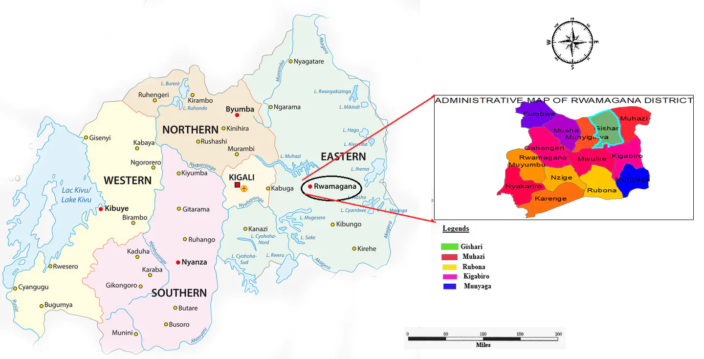
The study was conducted at the IPRC Gishari farm in Gishari Sector, Rwamagana District, Eastern Province, Rwanda, at geographical coordinates 1°57'12.65" S and 30°26'19.12" E (, ; see Figure 2). The site has a slope ranging from 7% to 15%, annual precipitation below 1500 mm, and an altitude between 1480 m and 1550 m above sea level.
3.3. Materials Used
Soil physical and chemical analyses were conducted at the University of Rwanda Huye Soil Laboratory using the equipment and reagents listed in Table 3.
Table 3: List of materials and equipment used in the research.
| S.No | Materials Used |
|---|---|
| 1 | Hoe, auger, and shovel for soil sampling |
| 2 | Electronic balance |
| 3 | Atomic Absorption Spectrophotometer (AAS) machine |
| 4 | pH meter (pH probe, Hanna Model HI 9032) |
| 5 | Electrical conductivity meter (EC probe, Hanna Model HI 9032) |
| 6 | Nitric acid for titration processes |
| 7 | Refrigerators to cool heated soil samples |
| 8 | Measuring tape (meters) for plot dimensions |
| 9 | Water storage tank () |
| 10 | Pyrex beakers |
| 11 | Graduated cylinders for water volume measurement |
| 12 | Graduated pipettes |
| 13 | Chemical reagents |
| 14 | Laptop computer and statistical software (SPSS 22.0, STATA 13.0, MS Excel) |
| 15 | CROPWAT 8.0 software |
| 16 | Soil shaker (Roto) machine |
3.4. Methodology Adopted
3.4.1. Analysis of Weather Parameters on Crop Production
Thirty years of historical weather data (1989–2019)—comprising rainfall, wind speed, maximum and minimum temperatures, relative humidity, and sunshine duration—were obtained from the Rwanda Meteorological Agency for the Kazo substation.
4.4.2. Determination of Physical and Chemical Properties of Soil
3.4.2.1. Soil Sampling Procedures and Collection
Surface debris was cleared within a 10 cm radius around each sampling point, and a soil auger was rotated into the topsoil. Composite core samples (200 g each) were collected in triplicate across four experimental plots (Plots I, II, III, and IV, each divided into subplots A, B, and C), yielding 12 total soil samples.
3.4.2.2. Soil Bulk Density
The weight of each representative soil sample was measured on an electronic balance (in g), and its volume was determined in a cylindrical container ():
3.4.2.3. Soil Porosity
Soil porosity was determined gravimetrically by measuring the volume of water required to saturate the void spaces of a known volume of oven-dry soil:
3.4.2.4. Soil Texture
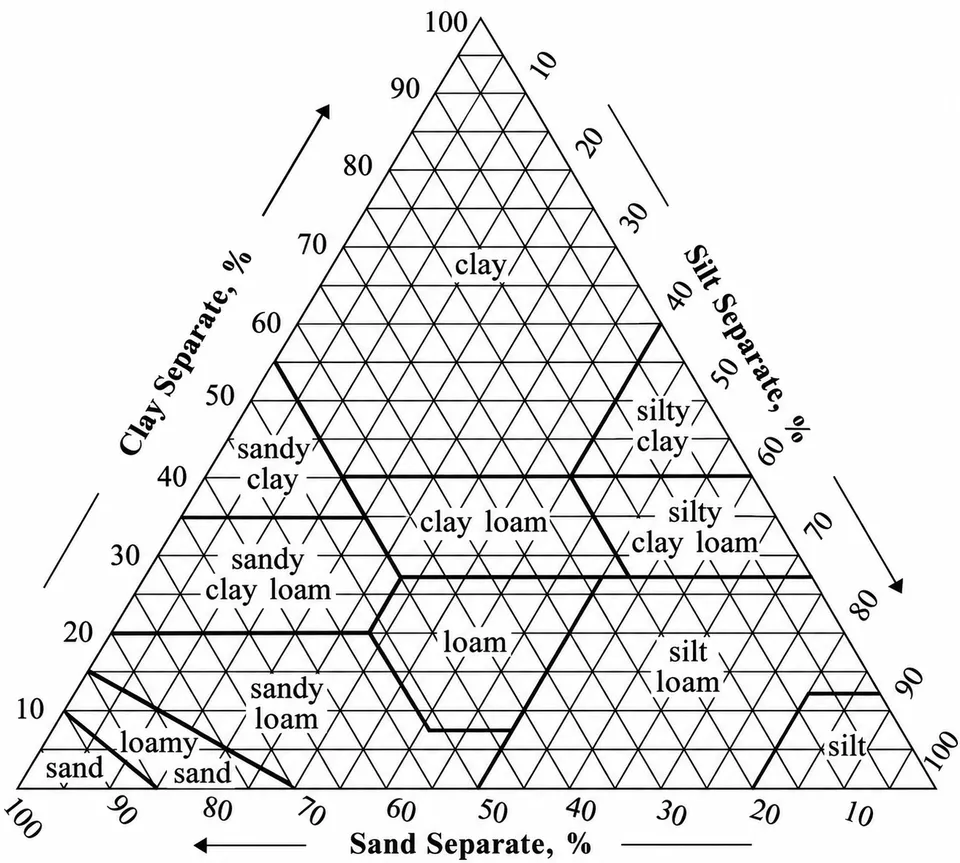
After removing coarse gravel (), 100 g of oven-dry soil was shaken for 5 minutes on a mechanical Roto sieve shaker to separate sand, silt, and clay fractions according to the particle size limits in Table 4 and classify the texture via the USDA textural triangle (see Figure 3).
Table 4: Classification of soil texture fractions based on particle size.
| Type of Particles | Size of Particles |
|---|---|
| Coarse material | |
| Sand | |
| Silt | |
| Clay |
3.4.2.5. Comparison of Soil Texture and Bulk Density Based on USDA-NRCS Guidelines
Measured bulk densities were evaluated against the USDA-NRCS root growth threshold guidelines presented in Table 2.
3.4.2.6. Soil pH
A 25 g soil sample was mixed with 25 mL of distilled water in a 100 mL beaker, stirred intermittently for 30 minutes, and measured with a Hanna Model HI 9032 pH meter calibrated with pH 7.0 and pH 4.0 buffer solutions.
3.4.2.7. Soil Electrical Conductivity (EC)
Forty grams (40 g) of soil were mixed with 80 mL of distilled water in a 200 mL flask, and electrical conductivity was measured using a Hanna Model HI 9032 conductivity meter calibrated against standard solution ( at 25 °C).
3.4.2.8. Determination of Calcium
A 10 mL soil extract aliquot was treated with 10 mL of potassium hydroxide, 1 mL of triethanolamine, potassium cyanide drops, and Cal-Red indicator, then titrated with EDTA from red to a blue endpoint.
3.4.2.9. Determination of Available Potassium
Plant-available potassium was extracted by mixing 5 g of soil with 25 mL of neutral ammonium acetate and quantified using a flame photometer calibrated between 0 and [88].
3.4.2.10. Soil Organic Matter Content (SOM)
Following the loss-on-ignition (LOI) procedure [81, 94, 96], 10 g of fresh soil () was dried at 105 °C for 3 hours to determine oven-dry weight () and gravimetric moisture content. The dried samples in pre-weighed crucibles () were combusted in a programmable muffle furnace (Koyo Lindberg Ltd, Model S1849) at 450 °C for 8 hours ():
3.4.2.11. Determination of Phosphorus
Five grams (5 g) of soil were shaken for 5 minutes in 50 mL of Bray No. 1 extractant and filtered. A 5 mL filtrate aliquot was reacted with 5 mL of molybdate reagent and 1 mL of dilute solution, diluted to 100 mL, and read after 10 minutes on a spectrophotometer at 660 nm against a calibration curve.
3.4.2.12. Total Nitrogen (TN)
Total nitrogen was determined via the Kjeldahl method (mineralization with concentrated sulfuric acid and catalyst at 300 °C for 2 hours, steam distillation with into boric acid, and titration to endpoint).
3.4.2.13. Sodium Adsorption Ratio (SAR)
The Sodium Adsorption Ratio () was computed from saturated paste extract ion concentrations (expressed in ):
3.4.3. Determination of Crop Water Requirement and Irrigation Scheduling of Carrot
3.4.3.1. Crop Water Requirements (CWR)
Crop evapotranspiration (, in ) was calculated by multiplying reference evapotranspiration () by the stage-specific crop coefficient () across the initial, development, mid-season, and late-season stages:
3.4.3.2. Irrigation Water Requirement (IR)
Daily root zone water depletion (, in mm) at the end of day was modeled in CROPWAT 8.0 using the water balance equation:
where is root zone depletion on day , is precipitation, is surface runoff, is net irrigation depth, is capillary rise from groundwater, is crop evapotranspiration, and is deep percolation (all in mm).
3.4.3.3. Irrigation Scheduling
CROPWAT 8.0 generated irrigation schedules specifying application dates, net and gross irrigation depths, and system flow rates assuming a baseline schedule efficiency.
3.4.4. Determination of Coefficient of Uniformity and Application Uniformity of Water
Drip irrigation uniformity was evaluated using Christiansen's Coefficient of Uniformity () and Keller and Karmeli's Emission Uniformity () [14, 17, 44, 47, 67, 68]:
where is the discharge of emitter , is the mean emitter discharge, is the number of emitters, is the average discharge of the lowest quartile (25%) of emitters, and is the coefficient of variation (). Field emission uniformity (, in %) was computed directly from the lowest-quartile average discharge (, in ) and overall average discharge (, in ) [47]:
3.5. Data Analysis and Processing
Descriptive statistics (mean, median, minimum, maximum, standard deviation, and coefficient of variation) were compiled in MS Excel, and one-way Analysis of Variance (ANOVA) with Duncan's post-hoc multiple range tests () was executed in SPSS 22.0 and STATA 13.0.
4. Results and Discussions
4.1. Weather Parameters of the Experimental Site
4.1.1. Rainfall at IPRC Gishari Farm Experimental Site
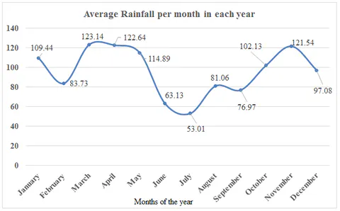
Based on the 30-year (1989–2019) monthly precipitation record shown in Figure 4, the highest average monthly rainfall occurred in March (123.14 mm), followed closely by April (122.64 mm) and November (121.54 mm). The lowest monthly rainfall occurred in July (53.01 mm) and June (63.13 mm), giving an annual range of 70.13 mm and a 12-month mean of 95.73 mm/month (1148.6 mm/year).
4.1.2. Minimum and Maximum Temperature at the Experimental Site
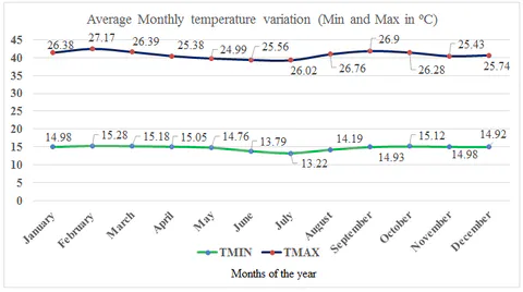
As shown in Figure 5, the 30-year mean monthly minimum temperature fluctuated between 13.22 °C (July) and 15.28 °C (February), with an annual average of 14.7 °C and a range of 2.06 °C. Mean monthly maximum temperature ranged from 24.99 °C (May) to 27.17 °C (February) and 26.9 °C (September), with an annual mean of 26.1 °C.
4.1.3. Relative Humidity at the Experimental Site
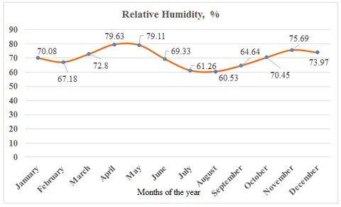
Mean monthly relative humidity ranged from a minimum of 60.53% in August (and 61.26% in July) to a maximum of 79.63% in April (and 79.11% in May), with an annual mean of 70.39% and a seasonal spread of 19.10% (see Figure 6).
4.1.4. Wind Speed at the Experimental Site
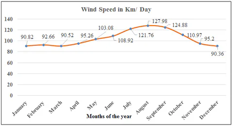
Mean daily wind speed peaked in August (127.98 km/day) and September (124.88 km/day), followed by July (121.76 km/day), and was lowest in December (90.36 km/day), March (90.52 km/day), and January (90.82 km/day), with an annual mean of 104.37 km/day and a range of 37.62 km/day (see Figure 7).
4.1.5. Sunshine Duration at the Experimental Site
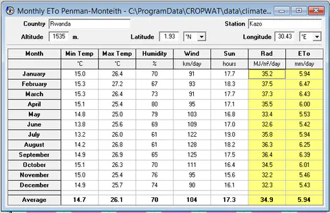
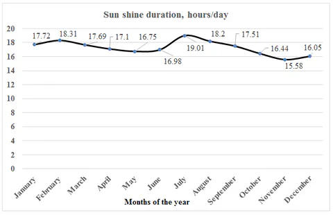
Mean daily sunshine duration peaked in July (19.01 hours/day) and February (18.31 hours/day), followed by August (18.2 hours/day), and was lowest in November (15.58 hours/day) and December (16.05 hours/day), averaging 17.28 hours/day across the year (see Figure 8). Corresponding solar radiation ranged from (November) to (February), with an annual average of .
4.2. Soil Properties at the Experimental Site
4.2.1. Determination of Soil Physical Properties of the Experimental Site
4.2.1.1. Soil Textural Classification Based on USDA Triangle
Across the 0.768 ha experimental area (), all four plots (Plots I–IV) were classified as sandy loam on the USDA textural triangle, with overall site averages of 68.16% sand, 22.43% silt, and 9.42% clay (see Table 5).
Table 5: Soil textural composition and USDA classification across experimental plots.
| Plot No | Statistic | Sand (%) | Silt (%) | Clay (%) | USDA Soil Texture |
|---|---|---|---|---|---|
| Plot I () | Mean ± SD | 70.619 ± 1.460 | 22.653 ± 4.494 | 6.728 ± 5.212 | Sandy Loam |
| Plot I () | Median (Min–Max) | 70.382 (69.291–72.183) | 22.623 (18.174–27.162) | 5.194 (2.456–12.535) | Sandy Loam |
| Plot I () | CV / Sum | 0.021 / 211.856 | 0.198 / 67.959 | 0.775 / 20.185 | Sandy Loam |
| Plot II () | Mean ± SD | 68.731 ± 2.306 | 21.268 ± 2.627 | 10.002 ± 1.142 | Sandy Loam |
| Plot II () | Median (Min–Max) | 68.175 (66.753–71.264) | 22.415 (18.262–23.126) | 10.474 (8.699–10.832) | Sandy Loam |
| Plot II () | CV / Sum | 0.034 / 206.192 | 0.124 / 63.803 | 0.114 / 30.005 | Sandy Loam |
| Plot III () | Mean ± SD | 68.864 ± 1.504 | 19.146 ± 1.954 | 11.990 ± 0.500 | Sandy Loam |
| Plot III () | Median (Min–Max) | 69.184 (67.226–70.182) | 19.015 (17.261–21.163) | 11.801 (11.611–12.557) | Sandy Loam |
| Plot III () | CV / Sum | 0.022 / 206.592 | 0.102 / 57.439 | 0.042 / 35.969 | Sandy Loam |
| Plot IV () | Mean ± SD | 64.414 ± 1.859 | 26.631 ± 3.947 | 8.955 ± 3.955 | Sandy Loam |
| Plot IV () | Median (Min–Max) | 64.163 (62.693–66.386) | 27.417 (22.351–30.126) | 7.181 (6.197–13.486) | Sandy Loam |
| Plot IV () | CV / Sum | 0.029 / 193.242 | 0.148 / 79.894 | 0.442 / 26.864 | Sandy Loam |
| Total Site () | Mean ± SD | 68.157 ± 2.845 | 22.425 ± 4.073 | 9.419 ± 3.463 | Sandy Loam |
| Total Site () | Median (Min–Max) | 68.680 (62.693–72.183) | 22.383 (17.261–30.126) | 10.653 (2.456–13.486) | Sandy Loam |
| Total Site () | CV / Sum | 0.042 / 817.882 | 0.182 / 269.095 | 0.368 / 113.023 | Sandy Loam |
4.2.1.2. Soil Bulk Density (BD) of the Experimental Site
Mean soil bulk density was in Plot I, in Plot II, in Plot III, and in Plot IV, with an overall experimental site mean of (see Table 6).
Table 6: Soil bulk density (BD) across the experimental plots.
| Plot No | Statistic | Initial Wt (g) | Area () | Height (cm) | Oven-Dry Wt (g) | Volume () | BD () |
|---|---|---|---|---|---|---|---|
| Plot I () | Mean ± SD | 200 ± 0.0 | 47.607 | 5.167 ± 0.306 | 137.160 ± 10.483 | 245.971 ± 14.544 | 0.815 ± 0.047 |
| Plot I () | Median (Min–Max) | 200 | 47.607 | 5.100 (4.90–5.50) | 139.700 (125.64–146.14) | 242.797 (233.28–261.84) | 0.824 (0.764–0.857) |
| Plot II () | Mean ± SD | 200 ± 0.0 | 47.607 | 3.500 ± 1.054 | 123.550 ± 5.629 | 166.626 ± 50.157 | 1.276 ± 0.385 |
| Plot II () | Median (Min–Max) | 200 | 47.607 | 3.400 (2.50–4.60) | 122.140 (118.76–129.75) | 161.865 (119.02–218.99) | 1.236 (0.913–1.680) |
| Plot III () | Mean ± SD | 200 ± 0.0 | 47.607 | 6.500 ± 0.656 | 135.357 ± 7.677 | 309.447 ± 31.218 | 0.651 ± 0.067 |
| Plot III () | Median (Min–Max) | 200 | 47.607 | 6.600 (5.80–7.10) | 132.130 (129.82–144.12) | 314.208 (276.12–338.01) | 0.637 (0.592–0.724) |
| Plot IV () | Mean ± SD | 200 ± 0.0 | 47.607 | 8.000 ± 0.964 | 128.660 ± 3.819 | 380.858 ± 45.911 | 0.531 ± 0.068 |
| Plot IV () | Median (Min–Max) | 200 | 47.607 | 8.400 (6.90–8.70) | 128.120 (125.14–132.72) | 399.901 (328.49–414.18) | 0.500 (0.483–0.609) |
| Total Site () | Mean ± SD | 200 ± 0.0 | 47.607 | 5.792 ± 1.863 | 131.182 ± 8.440 | 275.726 ± 88.705 | 0.818 ± 0.341 |
| Total Site () | Min–Max (CV) | 200 | 47.607 | 2.500–8.700 (0.322) | 118.760–146.140 (0.064) | 119.018–414.184 (0.322) | 0.483–1.680 (0.417) |
4.2.1.3. Soil Porosity of the Experimental Site
Mean soil porosity was 9.496% in Plot I, 14.592% in Plot II, 13.734% in Plot III, and 11.460% in Plot IV, resulting in an overall experimental site porosity of (range 6.175% to 17.083%; see Table 7).
Table 7: Determination of soil porosity across the experimental site.
| Plot No | Statistic | (g) | Dry Soil (g) | () (g) | Saturated (g) | Void Water (g) | Porosity (%) |
|---|---|---|---|---|---|---|---|
| Plot I () | Mean ± SD | 200 | 137.160 ± 10.483 | 337.160 ± 10.483 | 372.587 ± 3.470 | 35.427 ± 12.315 | 9.496 ± 3.265 |
| Plot I () | Median (Min–Max) | 200 | 139.700 (125.64–146.14) | 339.700 (325.64–346.14) | 373.020 (368.92–375.82) | 36.120 (22.78–47.38) | 9.611 (6.175–12.702) |
| Plot II () | Mean ± SD | 200 | 125.220 ± 5.744 | 325.220 ± 5.744 | 380.797 ± 1.717 | 55.577 ± 6.636 | 14.592 ± 1.706 |
| Plot II () | Median (Min–Max) | 200 | 127.150 (118.76–129.75) | 327.150 (318.76–329.75) | 381.180 (378.92–382.29) | 55.140 (49.17–62.42) | 14.424 (12.976–16.375) |
| Plot III () | Mean ± SD | 200 | 131.293 ± 19.829 | 331.293 ± 19.829 | 384.180 ± 20.312 | 52.887 ± 15.847 | 13.734 ± 3.792 |
| Plot III () | Median (Min–Max) | 200 | 134.280 (110.14–149.46) | 334.280 (310.14–349.46) | 386.640 (362.75–403.15) | 52.610 (37.18–68.87) | 14.503 (9.616–17.083) |
| Plot IV () | Mean ± SD | 200 | 131.990 ± 4.045 | 331.990 ± 4.045 | 375.097 ± 6.810 | 43.107 ± 10.727 | 11.460 ± 2.645 |
| Plot IV () | Median (Min–Max) | 200 | 131.420 (128.26–136.29) | 331.420 (328.26–336.29) | 373.570 (369.18–382.54) | 42.150 (32.89–54.28) | 11.283 (8.909–14.189) |
| Total Site () | Mean ± SD | 200 | 131.416 ± 10.955 | 331.416 ± 10.955 | 378.165 ± 10.439 | 46.749 ± 13.125 | 12.321 ± 3.269 |
| Total Site () | Median (Min–Max) | 200 | 130.585 (110.14–149.46) | 330.585 (310.14–349.46) | 377.370 (362.75–403.15) | 48.275 (22.78–68.87) | 12.839 (6.175–17.083) |
Note: = weight of beaker; = weight of dry soil; ; = weight of beaker, dry soil, and water at field capacity; ; .
4.2.1.4. Comparison of Studied Soil Bulk Density Based on USDA Triangle
Comparing the experimental plot bulk densities against USDA-NRCS thresholds confirms that all four sandy loam plots have average bulk densities (, overall mean ) well below the threshold, indicating ideal conditions for carrot root growth without compaction restrictions (see Table 8).
Table 8: Evaluation of experimental plot bulk densities against USDA-NRCS root growth thresholds.
| Plot | Soil Texture | Range of Plot BD () | Average Plot BD () | USDA Ideal BD () | USDA BD Affecting Roots () | USDA BD Restricting Roots () | Evaluation Decision |
|---|---|---|---|---|---|---|---|
| Plot I | Sandy loam | 0.764–0.857 | 0.815 | Ideal for plant growth | |||
| Plot II | Sandy loam | 0.913–1.680 | 1.276 | Ideal for plant growth | |||
| Plot III | Sandy loam | 0.592–0.724 | 0.651 | Ideal for plant growth | |||
| Plot IV | Sandy loam | 0.483–0.609 | 0.531 | Ideal for plant growth | |||
| All Plots | Sandy loam | 0.483–1.680 | 0.818 | Ideal for plant growth |
4.2.1.5. Soil Moisture and Soil Organic Matter of the Experimental Site
Gravimetric soil moisture content (MC) across all plots ranged from 16.50% to 58.80%, with an overall mean of (see Table 9). Soil organic matter (SOM) determined via loss on ignition ranged from 10.92% to 50.54%, with an overall mean of [95].
Table 9: Soil moisture content (MC) and soil organic matter (SOM) across experimental plots.
| Plot No | Statistic | Initial Wt (g) | Dry Wt (g) | MC (%) | Crucible (g) | @ 105 °C (g) | @ 450 °C (g) | SOM (%) |
|---|---|---|---|---|---|---|---|---|
| Plot I () | Mean ± SD | 10 | 6.030 ± 2.145 | 39.700 ± 21.446 | 33.243 ± 0.768 | 39.273 ± 1.611 | 25.320 ± 8.436 | 36.028 ± 18.499 |
| Plot I () | Median (Min–Max) | 10 | 5.620 (4.12–8.35) | 43.800 (16.50–58.80) | 32.820 (32.78–34.13) | 38.440 (38.25–41.13) | 22.160 (18.92–34.88) | 42.352 (15.20–50.54) |
| Plot II () | Mean ± SD | 10 | 6.777 ± 0.539 | 32.233 ± 5.395 | 33.853 ± 3.262 | 40.630 ± 2.951 | 33.983 ± 2.586 | 16.098 ± 8.053 |
| Plot II () | Median (Min–Max) | 10 | 6.920 (6.18–7.23) | 30.800 (27.70–38.20) | 35.290 (30.12–36.15) | 41.470 (37.35–43.07) | 32.870 (32.14–36.94) | 11.995 (10.92–25.38) |
| Plot III () | Mean ± SD | 10 | 5.887 ± 0.931 | 41.133 ± 9.309 | 31.733 ± 1.510 | 37.620 ± 2.153 | 28.727 ± 4.307 | 23.870 ± 7.939 |
| Plot III () | Median (Min–Max) | 10 | 5.840 (4.98–6.84) | 41.600 (31.60–50.20) | 31.870 (30.16–33.17) | 38.710 (35.14–39.01) | 29.280 (24.17–32.73) | 24.942 (15.45–31.22) |
| Plot IV () | Mean ± SD | 10 | 6.407 ± 0.911 | 35.933 ± 9.106 | 32.823 ± 2.050 | 39.230 ± 1.875 | 29.910 ± 2.574 | 23.778 ± 4.862 |
| Plot IV () | Median (Min–Max) | 10 | 6.290 (5.56–7.37) | 37.100 (26.30–44.40) | 32.810 (30.78–34.88) | 40.180 (37.07–40.44) | 28.750 (28.12–32.86) | 24.144 (18.74–28.45) |
| Total Site () | Mean ± SD | 10 | 6.275 ± 1.153 | 37.250 ± 11.525 | 32.913 ± 1.968 | 39.188 ± 2.186 | 29.485 ± 5.403 | 24.943 ± 12.054 |
| Total Site () | Median (Min–Max) | 10 | 6.235 (4.12–8.35) | 37.650 (16.50–58.80) | 32.815 (30.12–36.15) | 38.860 (35.14–43.07) | 30.710 (18.92–36.94) | 24.543 (10.92–50.54) |
Note: = initial soil weight; = oven-dry soil weight; = crucible weight; = crucible + dried soil at 105 °C; = crucible + combusted soil at 450 °C.
4.2.2. Determination of Soil Chemical Properties of the Experimental Site
4.2.2.1. Soil Chemical Properties (Ca, Mg, Na, K, and N)
Across all four experimental plots (see Table 10), mean concentrations were as follows:
- Calcium (): (range , ).
- Magnesium (): (range , ).
- Sodium (): (range , ).
- Potassium (): (range , ).
- Nitrogen (): (range , ).
- Soil Temperature: (range , ).
Table 10: Soil chemical properties () and temperature across experimental plots.
| Plot No | Statistic | Ca (ppm) | Mg (ppm) | Na (ppm) | K (ppm) | N (ppm) | Temp (°C) |
|---|---|---|---|---|---|---|---|
| Plot I () | Mean ± SD | 0.919 ± 0.158 | 1.471 ± 1.028 | 1.101 ± 0.116 | 0.652 ± 0.173 | 2.157 ± 0.207 | 28.133 ± 1.763 |
| Plot I () | Median (Min–Max) | 0.883 (0.782–1.092) | 1.937 (0.292–2.183) | 1.128 (0.973–1.201) | 0.669 (0.472–0.816) | 2.163 (1.947–2.361) | 28.580 (26.19–29.63) |
| Plot II () | Mean ± SD | 0.919 ± 0.194 | 1.860 ± 0.212 | 1.087 ± 0.197 | 0.713 ± 0.323 | 1.219 ± 0.631 | 28.353 ± 0.921 |
| Plot II () | Median (Min–Max) | 0.937 (0.716–1.103) | 1.911 (1.628–2.042) | 1.173 (0.862–1.227) | 0.729 (0.382–1.027) | 0.972 (0.749–1.937) | 28.520 (27.36–29.18) |
| Plot III () | Mean ± SD | 0.845 ± 0.041 | 1.758 ± 0.642 | 1.052 ± 0.076 | 1.105 ± 0.215 | 2.027 ± 0.890 | 28.770 ± 0.635 |
| Plot III () | Median (Min–Max) | 0.826 (0.817–0.892) | 1.451 (1.328–2.496) | 1.042 (0.981–1.132) | 1.182 (0.862–1.271) | 2.172 (1.073–2.835) | 28.930 (28.07–29.31) |
| Plot IV () | Mean ± SD | 0.923 ± 0.163 | 1.254 ± 0.509 | 0.950 ± 0.186 | 0.734 ± 0.427 | 1.680 ± 0.618 | 28.547 ± 0.673 |
| Plot IV () | Median (Min–Max) | 1.012 (0.735–1.021) | 1.072 (0.862–1.829) | 0.962 (0.758–1.129) | 0.627 (0.371–1.205) | 1.892 (0.984–2.163) | 28.620 (27.84–29.18) |
| Total Site () | Mean ± SD | 0.901 ± 0.133 | 1.586 ± 0.620 | 1.047 ± 0.144 | 0.801 ± 0.317 | 1.771 ± 0.661 | 28.451 ± 0.967 |
| Total Site () | Median (Min–Max) | 0.888 (0.716–1.103) | 1.729 (0.292–2.496) | 1.085 (0.758–1.227) | 0.773 (0.371–1.271) | 1.942 (0.749–2.835) | 28.600 (26.19–29.63) |
| Total Site () | CV / Sum | 0.147 / 10.816 | 0.391 / 19.031 | 0.137 / 12.568 | 0.396 / 9.613 | 0.373 / 21.248 | 0.034 / 341.410 |
Note: is parts per million, equivalent to .
4.2.2.2. Soil Acidity, Salinity, and Alkalinity of the Experimental Site
Across the experimental plots (see Table 11), mean soil pH was (range , ), indicating slightly acidic to near-neutral conditions [89]. Mean electrical conductivity (EC) was (range , ), classifying the soil as moderately saline. Mean Sodium Adsorption Ratio (SAR) was (range , ) [93].
Table 11: Soil acidity (pH), salinity (EC), and alkalinity (SAR) across experimental plots.
| Plot No | Statistic | pH | EC () | SAR |
|---|---|---|---|---|
| Plot I () | Mean ± SD | 6.497 ± 0.206 | 86.51 ± 7.135 | 0.382 ± 0.121 |
| Plot I () | Median (Min–Max) | 6.52 (6.28–6.69) | 88.32 (78.64–92.56) | 0.332 (0.295–0.520) |
| Plot II () | Mean ± SD | 7.033 ± 0.265 | 69.87 ± 2.737 | 0.330 ± 0.077 |
| Plot II () | Median (Min–Max) | 7.15 (6.73–7.22) | 70.62 (66.84–72.16) | 0.340 (0.248–0.401) |
| Plot III () | Mean ± SD | 6.973 ± 0.159 | 71.70 ± 2.166 | 0.329 ± 0.020 |
| Plot III () | Median (Min–Max) | 6.93 (6.84–7.15) | 71.76 (69.51–73.84) | 0.325 (0.311–0.350) |
| Plot IV () | Mean ± SD | 7.217 ± 0.049 | 68.36 ± 2.236 | 0.322 ± 0.020 |
| Plot IV () | Median (Min–Max) | 7.24 (7.16–7.25) | 68.27 (66.17–70.64) | 0.333 (0.300–0.334) |
| Total Site () | Mean ± SD | 6.930 ± 0.320 | 74.11 ± 8.354 | 0.341 ± 0.067 |
| Total Site () | Median (Min–Max) | 7.04 (6.28–7.25) | 71.20 (66.17–92.56) | 0.333 (0.248–0.520) |
| Total Site () | CV / Sum | 0.046 / 83.16 | 0.113 / 889.3 | 0.197 / 4.089 |
4.2.3. Analysis of Variance of Soil Physical and Chemical Properties
4.2.3.1. Analysis of Variance (ANOVA) of Soil Physical Properties
One-way ANOVA across the four plots revealed statistically significant differences at the 5% level for sand percentage (, ) and bulk density (, ), whereas silt (), clay (), porosity (), moisture content (), and SOM () did not differ significantly between plots (see Table 12).
Table 12: One-way Analysis of Variance (ANOVA) of soil physical properties across plots.
| Parameter | Source of Variation | Sum of Squares | df | Mean Square | Sig. (-value) | |
|---|---|---|---|---|---|---|
| Sand (%) | Between Groups | 62.70 | 3 | 20.90 | 6.347 | 0.016** |
| Sand (%) | Within Groups | 26.34 | 8 | 3.292 | — | — |
| Sand (%) | Total | 89.04 | 11 | — | — | — |
| Silt (%) | Between Groups | 89.50 | 3 | 29.83 | 2.567 | 0.127 ns |
| Silt (%) | Within Groups | 92.99 | 8 | 11.62 | — | — |
| Silt (%) | Total | 182.50 | 11 | — | — | — |
| Clay (%) | Between Groups | 43.21 | 3 | 14.40 | 1.299 | 0.340 ns |
| Clay (%) | Within Groups | 88.72 | 8 | 11.09 | — | — |
| Clay (%) | Total | 131.90 | 11 | — | — | — |
| Bulk Density () | Between Groups | 0.962 | 3 | 0.321 | 8.026 | 0.009** |
| Bulk Density () | Within Groups | 0.320 | 8 | 0.040 | — | — |
| Bulk Density () | Total | 1.282 | 11 | — | — | — |
| Porosity (%) | Between Groups | 47.63 | 3 | 15.88 | 1.817 | 0.222 ns |
| Porosity (%) | Within Groups | 69.89 | 8 | 8.737 | — | — |
| Porosity (%) | Total | 117.50 | 11 | — | — | — |
| MC (%) | Between Groups | 144.00 | 3 | 47.98 | 0.291 | 0.831 ns |
| MC (%) | Within Groups | 1317.00 | 8 | 164.70 | — | — |
| MC (%) | Total | 1461.00 | 11 | — | — | — |
| SOM (%) | Between Groups | 610.80 | 3 | 203.60 | 1.649 | 0.254 ns |
| SOM (%) | Within Groups | 987.50 | 8 | 123.40 | — | — |
| SOM (%) | Total | 1598.00 | 11 | — | — | — |
Note: ** indicates significance at the 5% level (); ns = not significant.
4.2.3.2. Analysis of Variance (ANOVA) of Soil Chemical Properties
One-way ANOVA of soil macronutrients and temperature indicated no statistically significant differences () between plots for (), (), (), (), (), or soil temperature (; see Table 13).
Table 13: One-way Analysis of Variance (ANOVA) of soil chemical properties across plots.
| Parameter | Source of Variation | Sum of Squares | df | Mean Square | Sig. (-value) | |
|---|---|---|---|---|---|---|
| Ca (ppm) | Between Groups | 0.013 | 3 | 0.004 | 0.187 | 0.902 ns |
| Ca (ppm) | Within Groups | 0.182 | 8 | 0.023 | — | — |
| Ca (ppm) | Total | 0.194 | 11 | — | — | — |
| Mg (ppm) | Between Groups | 0.685 | 3 | 0.228 | 0.515 | 0.683 ns |
| Mg (ppm) | Within Groups | 3.545 | 8 | 0.443 | — | — |
| Mg (ppm) | Total | 4.230 | 11 | — | — | — |
| Na (ppm) | Between Groups | 0.042 | 3 | 0.014 | 0.604 | 0.630 ns |
| Na (ppm) | Within Groups | 0.185 | 8 | 0.023 | — | — |
| Na (ppm) | Total | 0.227 | 11 | — | — | — |
| K (ppm) | Between Groups | 0.380 | 3 | 0.127 | 1.398 | 0.313 ns |
| K (ppm) | Within Groups | 0.726 | 8 | 0.091 | — | — |
| K (ppm) | Total | 1.106 | 11 | — | — | — |
| N (ppm) | Between Groups | 1.581 | 3 | 0.527 | 1.305 | 0.338 ns |
| N (ppm) | Within Groups | 3.230 | 8 | 0.404 | — | — |
| N (ppm) | Total | 4.811 | 11 | — | — | — |
| Temp (°C) | Between Groups | 0.664 | 3 | 0.221 | 0.184 | 0.904 ns |
| Temp (°C) | Within Groups | 9.627 | 8 | 1.203 | — | — |
| Temp (°C) | Total | 10.290 | 11 | — | — | — |
Note: ns = not significant at the 5% level.
4.2.3.3. One-Way ANOVA of Soil Acidity, Salinity, and Alkalinity
One-way ANOVA demonstrated statistically significant differences across plots for soil pH (, ) and electrical conductivity (EC) (, ), whereas SAR did not vary significantly between plots (, ; see Table 14).
Table 14: One-way ANOVA of soil acidity (pH), salinity (EC), and alkalinity (SAR) across plots.
| Parameter | Source of Variation | Sum of Squares | df | Mean Square | Sig. (-value) | |
|---|---|---|---|---|---|---|
| pH (unitless) | Between Groups | 0.848 | 3 | 0.283 | 8.041 | 0.008** |
| pH (unitless) | Within Groups | 0.281 | 8 | 0.035 | — | — |
| pH (unitless) | Total | 1.129 | 11 | — | — | — |
| EC () | Between Groups | 631.40 | 3 | 210.50 | 12.360 | 0.002** |
| EC () | Within Groups | 136.20 | 8 | 17.02 | — | — |
| EC () | Total | 767.60 | 11 | — | — | — |
| SAR | Between Groups | 0.007 | 3 | 0.002 | 0.440 | 0.731 ns |
| SAR | Within Groups | 0.043 | 8 | 0.005 | — | — |
| SAR | Total | 0.050 | 11 | — | — | — |
Note: ** indicates significance at the 5% level (); ns = not significant.
4.3. Assessment of Crop Water Requirement, Water Deficit, and Irrigation Scheduling of Carrot
4.3.1. Reference Evapotranspiration (ETo) under Carrot Crop
Using CROPWAT 8.0, mean reference evapotranspiration () at the experimental site was , ranging from a minimum of in June (and in December) to a maximum of in February (see Table 15).
Table 15: Monthly reference evapotranspiration () and climatic parameters computed via CROPWAT 8.0.
| Month | Min Temp (°C) | Max Temp (°C) | Humidity (%) | Wind Speed (km/day) | Sunshine (hours) | Solar Radiation () | (mm/day) |
|---|---|---|---|---|---|---|---|
| January | 15.0 | 26.4 | 70 | 91 | 17.7 | 35.2 | 5.94 |
| February | 15.3 | 27.2 | 67 | 93 | 18.3 | 37.5 | 6.47 |
| March | 15.3 | 26.4 | 73 | 91 | 17.7 | 37.3 | 6.43 |
| April | 15.1 | 25.4 | 80 | 95 | 17.1 | 35.5 | 6.00 |
| May | 14.8 | 25.0 | 79 | 103 | 16.8 | 33.4 | 5.53 |
| June | 13.8 | 25.6 | 69 | 109 | 17.0 | 32.6 | 5.42 |
| July | 13.2 | 26.0 | 61 | 122 | 19.0 | 35.8 | 5.94 |
| August | 14.2 | 26.8 | 61 | 128 | 18.2 | 36.3 | 6.25 |
| September | 14.9 | 26.9 | 65 | 125 | 17.5 | 36.4 | 6.39 |
| October | 15.1 | 26.3 | 70 | 111 | 16.4 | 34.5 | 6.01 |
| November | 15.0 | 25.4 | 76 | 95 | 15.6 | 32.2 | 5.46 |
| December | 14.9 | 25.7 | 74 | 90 | 16.1 | 32.3 | 5.43 |
| Average | 14.7 | 26.1 | 70 | 104 | 17.3 | 34.9 | 5.94 |
4.3.2. Crop Water Requirement (CWR) of Carrot
4.3.2.1. Effective Rainfall (Eff. Rain) of the Experimental Site
Total annual rainfall was 1148.6 mm, of which 962.6 mm was effective rainfall stored in the root zone (see Table 16). Monthly effective rainfall ranged from a minimum of 48.5 mm in July to a maximum of 98.9 mm in March.
Table 16: Monthly total rainfall and effective rainfall at the experimental site.
| Month | (mm/day) | Total Rain (mm) | Effective Rain (mm) |
|---|---|---|---|
| January | 5.94 | 109.4 | 90.3 |
| February | 6.47 | 83.7 | 72.5 |
| March | 6.43 | 123.1 | 98.9 |
| April | 6.00 | 122.6 | 98.6 |
| May | 5.53 | 114.9 | 93.8 |
| June | 5.42 | 63.1 | 56.7 |
| July | 5.94 | 53.0 | 48.5 |
| August | 6.25 | 81.1 | 70.6 |
| September | 6.39 | 77.0 | 67.5 |
| October | 6.01 | 102.1 | 85.4 |
| November | 5.46 | 121.5 | 97.9 |
| December | 5.43 | 97.1 | 82.0 |
| Total / Mean | 5.94 | 1148.6 | 962.6 |
4.3.2.2. Gross Irrigation (GI), Net Irrigation, and Water Deficit
Across the 100-day carrot growing season (16 May to 19 August), cumulative crop evapotranspiration () was 474.7 mm/season, effective rainfall was 207.1 mm/season, and the cumulative irrigation requirement was 273.2 mm (see Table 17). Normalized over the cultivated area (), the Net Irrigation Water Requirement (NIWR) was , the Gross Irrigation Water Requirement (GIWR) was , and total water losses (deficit) were .
Table 17: Decadal crop water requirement, effective rainfall, and net/gross irrigation requirements for carrot (16 May to 19 August).
| Month | Decade | Stage | (mm/day) | (mm/dec) | Eff. Rain (mm/dec) | Irr. Req. (mm/dec) | |
|---|---|---|---|---|---|---|---|
| May | 2 | Init | 0.45 | 2.49 | 22.4 | 29.5 | 0.00 |
| May | 3 | Init | 0.45 | 2.47 | 27.2 | 28.1 | 0.00 |
| June | 1 | Deve | 0.56 | 3.04 | 30.4 | 22.1 | 8.30 |
| June | 2 | Deve | 0.75 | 4.07 | 40.7 | 17.6 | 23.10 |
| June | 3 | Deve | 0.95 | 5.29 | 52.9 | 17.1 | 35.80 |
| July | 1 | Mid | 1.03 | 5.95 | 59.5 | 16.1 | 43.40 |
| July | 2 | Mid | 1.03 | 6.13 | 61.3 | 14.8 | 46.50 |
| July | 3 | Late | 1.03 | 6.23 | 68.6 | 17.7 | 50.90 |
| August | 1 | Late | 0.98 | 6.05 | 60.5 | 21.8 | 38.60 |
| August | 2 | Late | 0.91 | 5.70 | 51.3 | 22.2 | 26.60 |
| Total | — | — | — | — | 474.7 | 207.1 | 273.2 |
Note: ; ; .
4.3.2.3. Irrigation Scheduling of the Experimental Site
The CROPWAT 8.0 irrigation schedule across the 100-day season (16 May to 19 August) is detailed in Table 18. Root zone moisture depletion at irrigation events ranged from 32% to 66% (mean 54.5%), net irrigation depths ranged from 10.00 mm to 23.80 mm (total 351.10 mm), and gross irrigation depths ranged from 14.20 mm to 34.00 mm (total 501.60–501.70 mm), with field flow rates ranging from to [75].
Table 18: CROPWAT 8.0 irrigation schedule for carrot from 16 May to 19 August.
| Date | Day | Stage | Rain (mm) | (fract.) | (%) | Depl. (%) | Net Irr. (mm) | Deficit (mm) | Loss (mm) | Gross Irr. (mm) | Flow (L/s/ha) |
|---|---|---|---|---|---|---|---|---|---|---|---|
| 16-May | 5 | Init | 0.00 | 1.00 | 100.00 | 50.00 | 10.00 | 0.00 | 0.00 | 14.20 | 0.33 |
| 21-May | 10 | Init | 0.00 | 1.00 | 100.00 | 57.00 | 12.40 | 0.00 | 0.00 | 17.80 | 0.41 |
| 1-Jun | 21 | Dev | 0.00 | 1.00 | 100.00 | 60.00 | 15.40 | 0.00 | 0.00 | 22.00 | 0.23 |
| 11-Jun | 31 | Dev | 0.00 | 1.00 | 100.00 | 55.00 | 16.20 | 0.00 | 0.00 | 23.20 | 0.27 |
| 16-Jun | 36 | Dev | 0.00 | 1.00 | 100.00 | 52.00 | 16.30 | 0.00 | 0.00 | 23.30 | 0.54 |
| 21-Jun | 41 | Dev | 0.00 | 1.00 | 100.00 | 65.00 | 21.60 | 0.00 | 0.00 | 30.80 | 0.71 |
| 26-Jun | 46 | Dev | 0.00 | 1.00 | 100.00 | 61.00 | 21.10 | 0.00 | 0.00 | 30.20 | 0.70 |
| 30-Jun | 50 | Dev | 0.00 | 1.00 | 100.00 | 58.00 | 21.10 | 0.00 | 0.00 | 30.20 | 0.87 |
| 5-Jul | 55 | Mid | 0.00 | 1.00 | 100.00 | 58.00 | 21.00 | 0.00 | 0.00 | 30.00 | 0.69 |
| 10-Jul | 60 | Mid | 0.00 | 1.00 | 100.00 | 66.00 | 23.80 | 0.00 | 0.00 | 34.00 | 0.79 |
| 15-Jul | 65 | Mid | 0.00 | 1.00 | 100.00 | 63.00 | 22.70 | 0.00 | 0.00 | 32.50 | 0.75 |
| 19-Jul | 69 | Mid | 0.00 | 1.00 | 100.00 | 51.00 | 18.40 | 0.00 | 0.00 | 26.30 | 0.76 |
| 22-Jul | 72 | Mid | 0.00 | 1.00 | 100.00 | 51.00 | 18.60 | 0.00 | 0.00 | 26.60 | 1.03 |
| 25-Jul | 75 | Mid | 0.00 | 1.00 | 100.00 | 52.00 | 18.70 | 0.00 | 0.00 | 26.70 | 1.03 |
| 29-Jul | 79 | Mid | 0.00 | 1.00 | 100.00 | 52.00 | 18.70 | 0.00 | 0.00 | 26.70 | 0.77 |
| 1-Aug | 82 | End | 0.00 | 1.00 | 100.00 | 51.00 | 18.50 | 0.00 | 0.00 | 26.40 | 1.02 |
| 5-Aug | 86 | End | 0.00 | 1.00 | 100.00 | 50.00 | 18.10 | 0.00 | 0.00 | 25.90 | 0.75 |
| 9-Aug | 90 | End | 0.00 | 1.00 | 100.00 | 50.00 | 18.10 | 0.00 | 0.00 | 25.90 | 0.75 |
| 15-Aug | 96 | End | 0.00 | 1.00 | 100.00 | 56.00 | 20.30 | 0.00 | 0.00 | 29.00 | 0.56 |
| 19-Aug | End | End | 0.00 | 1.00 | 0.00 | 32.00 | — | — | — | — | — |
| Total | — | — | — | — | — | — | 351.00 | 0.00 | 0.00 | 501.70 | 12.96 |
Note: Seasonal summary parameters: Total gross irrigation = 501.60 mm; Total net irrigation = 351.10 mm; Total irrigation losses = 0.00 mm; Actual water use by crop = 469 mm; Potential water use by crop = 469 mm; Efficiency of irrigation schedule = 100%; Deficiency of irrigation schedule = 0.00%; Total rainfall = 243.9 mm; Effective rainfall = 107.9 mm; Total rain loss = 136 mm; Moisture deficit at harvest = 11.4 mm; Actual irrigation requirement = 361 mm; Rain efficiency = 44.3%.
4.4. Assessment of the Uniformity Coefficient of Water under the Drip Irrigation System
4.4.1. Computation of Emitter Discharge at the Experimental Site
Field discharge measurements of the inline drippers across three replications (RI, RII, RIII) in Plots I–IV yielded an overall mean emitter discharge rate of (range , ; see Table 19).
Table 19: Computation of emitter discharge rates () across experimental plots.
| Plot No | Statistic | Replication I (L/h) | Replication II (L/h) | Replication III (L/h) | Average Discharge (L/h) |
|---|---|---|---|---|---|
| Plot I () | Mean ± SD | 2.487 ± 0.335 | 1.833 ± 0.165 | 1.883 ± 0.573 | 2.067 ± 0.239 |
| Plot I () | Min–Max (CV) | 2.160–2.830 (0.135) | 1.650–1.970 (0.090) | 1.280–2.420 (0.304) | 1.800–2.260 (0.115) |
| Plot II () | Mean ± SD | 2.640 ± 0.347 | 2.157 ± 0.630 | 2.460 ± 0.248 | 2.420 ± 0.331 |
| Plot II () | Min–Max (CV) | 2.260–2.940 (0.131) | 1.730–2.880 (0.292) | 2.270–2.740 (0.101) | 2.130–2.780 (0.137) |
| Plot III () | Mean ± SD | 2.690 ± 0.395 | 2.090 ± 0.111 | 2.230 ± 0.272 | 2.340 ± 0.082 |
| Plot III () | Min–Max (CV) | 2.240–2.980 (0.147) | 1.970–2.190 (0.053) | 1.980–2.520 (0.122) | 2.270–2.430 (0.035) |
| Plot IV () | Mean ± SD | 2.323 ± 0.275 | 2.313 ± 0.295 | 2.160 ± 0.195 | 2.263 ± 0.195 |
| Plot IV () | Min–Max (CV) | 2.150–2.640 (0.118) | 1.980–2.540 (0.127) | 1.970–2.360 (0.090) | 2.040–2.400 (0.086) |
| Total Site () | Mean ± SD | 2.535 ± 0.327 | 2.098 ± 0.358 | 2.183 ± 0.371 | 2.273 ± 0.239 |
| Total Site () | Median (Min–Max) | 2.555 (2.150–2.980) | 1.975 (1.650–2.880) | 2.230 (1.280–2.740) | 2.295 (1.800–2.780) |
| Total Site () | CV / Sum | 0.129 / 30.420 | 0.170 / 25.180 | 0.170 / 26.200 | 0.105 / 27.270 |
4.4.2. Parameters of Drip Irrigation Performance Evaluation
As shown in Table 20, the overall mean Christiansen's Uniformity Coefficient () was (range ), exceeding the 80% threshold for excellent performance [7]. Furthermore, overall Emission Uniformity () averaged across the site (ranging from 87.097% in Plot I to 97.009% in Plot III), exceeding the 90% ASAE threshold for excellent emission uniformity [2, 63].
Table 20: Drip irrigation uniformity parameters across experimental plots.
| Plot No | Statistic | Average (L/h) | CUC (%) | CV (%) | EU or DU (%) |
|---|---|---|---|---|---|
| Plot I () | Mean ± SD | 2.067 ± 0.239 | 79.777 ± 23.595 | 311.564 ± 384.863 | 87.097 |
| Plot I () | Min–Max | 1.800–2.260 | 53.330–98.670 | 17.056–747.034 | 87.097 |
| Plot II () | Mean ± SD | 2.420 ± 0.331 | 75.777 ± 23.404 | 271.212 ± 228.788 | 88.017 |
| Plot II () | Min–Max | 2.130–2.780 | 49.000–92.330 | 94.311–529.584 | 88.017 |
| Plot III () | Mean ± SD | 2.340 ± 0.082 | 93.110 ± 7.907 | 82.922 ± 93.555 | 97.009 |
| Plot III () | Min–Max | 2.270–2.430 | 84.330–99.670 | 4.245–186.370 | 97.009 |
| Plot IV () | Mean ± SD | 2.263 ± 0.195 | 85.333 ± 7.426 | 192.884 ± 114.540 | 90.133 |
| Plot IV () | Min–Max | 2.040–2.400 | 77.330–92.000 | 98.272–320.227 | 90.133 |
| Total Site () | Mean ± SD | 2.273 ± 0.239 | 83.499 ± 16.382 | 214.645 ± 220.727 | 93.949 |
| Total Site () | Min–Max (P25–P75) | 1.800–2.780 (2.135–2.375) | 49.000–99.670 (80.83–93.83) | 4.245–747.034 (76.23–254.98) | 93.949 |
4.4.2.1. Application Efficiency for the Drip Irrigation System
Field application efficiency () relating net root-zone storage () to gross water delivered () was computed as:
Consequently, corresponds to system water losses.
4.5. Estimation of Carrot Yield under Drip Irrigation in Experimental Plots
The ( or ) experimental field was divided into four main plots, each containing three subplots measuring ( or ; see Figure 9).
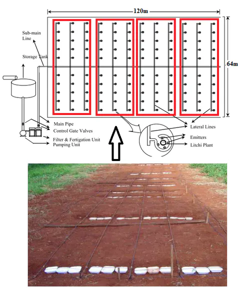
As summarized in Table 21, carrot yield per subplot averaged (range ), yielding a total harvest of () across the experimental area, equivalent to approximately .
Table 21: Carrot yield across the experimental plots under drip irrigation.
| Plot No | Statistic | Total Farm Size (ha) | Subplot Area (ha) | Productivity (kg/subplot) |
|---|---|---|---|---|
| Plot I () | Mean ± SD | 0.768 | 0.048 | 326.910 ± 37.285 |
| Plot I () | Median (Min–Max) | 0.768 | 0.048 | 315.450 (296.700–368.580) |
| Plot I () | Variance / CV | 0.000 | 0.000 | 1390.182 / 0.114 |
| Plot II () | Mean ± SD | 0.768 | 0.048 | 321.430 ± 23.576 |
| Plot II () | Median (Min–Max) | 0.768 | 0.048 | 320.150 (298.520–345.620) |
| Plot II () | Variance / CV | 0.000 | 0.000 | 555.831 / 0.073 |
| Plot III () | Mean ± SD | 0.768 | 0.048 | 306.673 ± 8.258 |
| Plot III () | Median (Min–Max) | 0.768 | 0.048 | 310.120 (297.250–312.650) |
| Plot III () | Variance / CV | 0.000 | 0.000 | 68.200 / 0.027 |
| Plot IV () | Mean ± SD | 0.768 | 0.048 | 317.263 ± 16.336 |
| Plot IV () | Median (Min–Max) | 0.768 | 0.048 | 325.150 (298.480–328.160) |
| Plot IV () | Variance / CV | 0.000 | 0.000 | 266.875 / 0.051 |
| Total Site () | Mean ± SD | 0.768 | 0.048 | 318.069 ± 21.788 |
| Total Site () | Median (Min–Max) | 0.768 | 0.048 | 314.050 (296.700–368.580) |
| Total Site () | Variance / CV / Sum | 0.000 | 0.000 | 474.735 / 0.069 / 3816.83 |
5. Summary, Conclusion and Recommendations
5.1. Summary
This research evaluated the performance of a drip irrigation system on carrot production at the IPRC Gishari farm in Rwanda by analyzing 30-year historical weather parameters, soil physical and chemical properties across 12 subplots (four plots divided into three subplots each), CROPWAT 8.0 crop water requirements and scheduling, emitter discharge uniformity, and carrot harvest yields.
5.2. Conclusions
- Objective 1 (Weather Parameters): Over the 30-year record (1989–2019), average monthly precipitation peaked in March (123.14 mm) and April (122.64 mm) and was lowest in July (53.01 mm). Mean monthly minimum temperatures ranged between 13.22 °C (July) and 15.28 °C (February), while mean maximum temperatures ranged from 24.99 °C (May) to 27.17 °C (February) and 26.9 °C (September). Relative humidity averaged 70.39% (ranging from 60.53% in August to 79.63% in April). Wind speed averaged 104.37 km/day (peaking at 127.98 km/day in August), and sunshine duration averaged 17.28 hours/day (ranging from 15.58 to 19.01 hours/day).
- Objective 2 (Soil Physical and Chemical Properties): The experimental site soil is classified as sandy loam (68.16% sand, 22.43% silt, 9.42% clay), with an overall mean bulk density of ( across plots, ideal for root growth under USDA-NRCS criteria) and a mean porosity of 12.32%. Mean gravimetric moisture content was 37.25% (16.5%–58.8%), and mean soil organic matter (SOM) was 24.94% (10.92%–50.54%). Mean chemical concentrations were , , , , and , with a mean soil temperature of 28.5 °C, a slightly acidic to neutral pH of 6.93 (6.28–7.25), moderate salinity (, range ), and low sodicity (, range ). One-way ANOVA confirmed statistically significant inter-plot differences () for sand percentage (), bulk density (), pH (), and EC ().
- Objective 3 (Crop Water Requirement and Scheduling): Mean solar radiation was (), and mean reference evapotranspiration () was (). Annual rainfall totaled 1148.6 mm, with 962.6 mm effective rainfall. For the 100-day carrot season (16 May to 19 August), the net irrigation requirement was , the gross irrigation requirement was , and water losses were . Under the CROPWAT 8.0 schedule, total net irrigation applied was 351.10 mm and gross irrigation was 501.60–501.70 mm at an average field flow rate of .
- Objective 4 (Drip Uniformity Evaluation): The drip system achieved an overall mean Christiansen's Uniformity Coefficient () of 83.5% (range 49.0%–99.7%) and an Emission Uniformity () of 93.9% (range 87.1%–97.0%), both rated as excellent under ASAE standards, while field application efficiency () was 54.45%.
- Objective 5 (Carrot Yield Assessment): Mean carrot yield was per subplot (), producing a total harvest of () across the experimental area, or approximately .
5.3. Recommendations
- The University of Rwanda (UR) and the College of Agriculture, Animal Sciences and Veterinary Medicine (CAVM) should equip soil and water laboratories with essential analytical instruments, chemical reagents, and streamlined procurement logistics to support graduate research, alongside training laboratory technicians in soil and water quality analysis.
- UR and CAVM should acquire advanced hydrological and hydraulic modeling software—including Arc Hydro Groundwater (AHGW), Groundwater Modeling System (GMS), Surface-water Modeling System (SMS), and Watershed Modeling System (WMS)—to enhance catchment water balance and irrigation system design.
5.3.1. Area for Further Research
Future studies should expand the sample size and spatial scale of soil physical and chemical property measurements across multiple agro-ecological zones to strengthen statistical power and reduce sampling bias.
Appendices