## I. INTRODUCTION The world economy today is in a global crisis. The COVID-19 coronavirus pandemic caused serious problems not only of a humanitarian nature, but also inevitably caused a significant slowdown in economic activity, which, in turn, gave rise to serious financial problems for enterprises and organizations in almost all sectors of modern world business. However, along with a sharp decrease in consumer demand and a corresponding decrease in GDP, each country, along with solving current socioeconomic problems, now sets itself another task: how to revive its economy in the current conditions so as to activate financial and economic activities with the least possible costs. Thus, ensuring the effectiveness of investments, which are inevitable when restoring the world economy destroyed by the pandemic, comes to the fore when solving the problem of resuscitation. From the point of view of system analysis, the restoration of the pre-crisis level of economic development consistently leads to the search for such financial investment instruments that, on the one hand, would be available in conditions of a significant decrease in the solvency of specific organizations, but, on the other hand, would allow us to quantify the effectiveness of invested funds. One of these tools, which, for sure, will be actively used in various sectors of modern business, is financial or operational leasing. This type of entrepreneurial activity is extremely widespread in the West (for example, in the United States, at least half of the loans for the development of the material and technical base of companies are carried out through a system of leasing relations), since, as a mechanism for indirect alternative investment, it is much more accessible to the end user (lessee) in financial terms. In addition, greater flexibility in the formation of conditions for the repayment of lease payments in an agreement with the lessor, as well as the use of tax benefits in this case, are additional advantages when using leasing operations. In countries with developed market economies, leasing accounts for almost a third of investment in fixed assets, and in other countries with high growth rates, this ratio is at least 10-15% (Drury 1990, Upneja 2001, Goodacre 2003, Shaoul 2007). In Russia, to date, leasing has not yet received a fairly wide application, however, the extraordinary modern economic conditions will only contribute to the use and development of various types of lease (Gazman 2011, 2013, 2017, 2019, Gerasimova 2018, Leontieva 2019, Podgornaya 2019, Litvinova 2020). This is confirmed by the proposals of the President of the Russian Federation on the use of leasing in the aviation and automotive industries, expressed by him in April 2020. In addition, the program for the development of the electronic industry of the Russian Federation, which is the basis of the entire modern technological base for the implementation of the most important national projects, emphasizes that the depreciation of fixed assets is estimated at $60 - 75\%$, but their renewal is constrained by the lack of available financial resources. The situation is approximately the same in mechanical engineering, a strategic branch of any economy. All of the above gives serious grounds to believe that the use and development of various types of leasing operations is a very relevant tool for solving the problem of resuscitation not only of the Russian, but also of the world economy. Quite a lot is known and written about the advantages of leasing for the lessee (Vecchi 2013, Chau 2014, Bulbul 2014, Zhang 2018, van Loon 2020), however, in order to realize these advantages, the end user obviously needs to have an obligatory intermediate link - the lessor - i.e., an organization that which actually makes it possible to implement the leasing operation. Thus, before evaluating the effectiveness of leasing for the lessee, it is absolutely necessary to consider the issue of efficiency for the lessor. ## II. FORMULATION OF THE PROBLEM Financial leasing, which is common in practice, assumes that an organization can acquire the necessary equipment not by purchasing, but by renting it from the lessor's company, which, in turn, can rent it or buy it from the manufacturer. The option when the lessor is the owner of the equipment can not be considered - its effectiveness is obvious. In the first case, the lessor, on the one hand, leases equipment from the manufacturer, and on the other hand, leases it to the lessee's enterprise. In the second case, the lessor buys the equipment from the manufacturer and leases it to the lessee's enterprise. Both of these options are schematically shown in Figure1. In both cases, the purchase and lease of equipment from the manufacturer can be realized both through the use of equity capital (EC) and through loan capital (LC), such as a bank loan. As a result, from the point of view of the lessor, we have 4 options for the implementation of leasing operations: 1. Investments (outflows) - lease payments to the manufacturer at the expense of the EC; income (inflows) - lease payments from the lessee's enterprise; 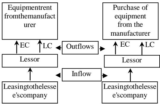 Figure 1: Leasing options for the lessor 2. Investment (outflows) - payments to the manufacturer for the purchase in installments at the expense of the EC; income (inflows) - lease payments from a lessee's enterprise; expense of the EC; income(inflows) - lease payments from a lessee's enterprise; 3. Investments (outflows) - lease payments to the manufacturer at the expense of the LC; income (inflows) - lease payments from a lessee's enterprise; 4. Investment (outflows) - payments to the manufacturer for the purchase in installments at the expense of the LC; income (inflows) - lease payments from a machine-building enterprise. Thus, the dynamics of leasing operations in the schemes of Figure 1 can be represented by investment projects, in which expenses are outflows, and incomes are inflows of the corresponding project. Then the efficiency of leasing for the lessor can be quantified using the known performance indicators: NPV (Net Present Value); DPI (Discounted Profitability Index); DPP (Discounted Payback Period); IRR (Internal Rate of Return). ## III. THE ORETICAL ANALYSIS The financial-time diagram for implementation of the operation of acquiring equipment by the lessor on a leasehold basis from the manufacturer (with its subsequent leasing to the lessee) is shown in figure 2. In figure 2: ST $[R_{\text{rent}}(t)]$ - stream of investment (rent) payments $R_{\text{rent}}(t)$ duration $n_{\text{rent}}$, which is determined by the terms of the contract with the manufacturer; ST $[R_{\text{leas.}}(t)]$ - income stream, the size of which $R_{\text{leas.}}(t)$ and their duration $n_{\text{leas}}$ is determined by the terms of the contract with the lessor. 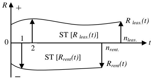 Figure 2: Financial-time diagram of the operation of leasing In figure 2: ST $[R_{\text{rent}}(t)]$ - stream of investment (rent) payments $R_{\text{rent}}(t)$ duration $n_{\text{rent}}$, which is determined by the terms of the contract with the manufacturer; ST $[R_{\text{leas.}}(t)]$ - income stream, the size of which $R_{\text{leas.}}(t)$ and their duration $n_{\text{leas}}$ is determined by the terms of the contract with the lessor. The indicators of economic efficiency of this operation as an investment project – net present value (NPV) and discounted profitability index (DPI) – are determined by obvious ratios based on the discounted approach of financial mathematics: $$ \mathrm{N P V} = \mathrm{P} _ {0} \left[ \mathrm{R} _ {\text{leas .}} (\mathrm{t}) \right] - \mathrm{P} _ {0} \left[ \mathrm{R} _ {\text{rent}} (\mathrm{t}) \right], \tag{1} $$ $$ \mathrm{DPI} = \frac{\mathrm{P} _ {0} \left[ \mathrm{R} _ {\text{leas .}} (\mathrm{t}) \right]}{\mathrm{P} _ {0} \left[ \mathrm{R} _ {\text{rent}} (\mathrm{t}) \right]}, \tag{2} $$ $\mathrm{P_0}\left[\mathrm{R}_{\mathrm{leas.}}(\mathrm{t})\right] = \sum_{\mathrm{t} = 0}^{\mathrm{n}_{\mathrm{leas.}}}\frac{\mathrm{R}_{\mathrm{leas.}}(\mathrm{t})}{(1 + \mathrm{r})^{\mathrm{t}}}$ -present value of the income payments at the beginning of the operation $(t = 0)$; rate of return for the lessor; $\mathrm{P_0}\left[\mathrm{R}_{\mathrm{rent}}(\mathrm{t})\right] = \sum_{\mathrm{t} = 0}^{\mathrm{n}_{\mathrm{rent}}}\frac{\mathrm{R}_{\mathrm{rent}}(\mathrm{t})}{(1 + \mathrm{i})^{\mathrm{t}}}$ - present value of the investment payments reduced to the beginning of the operation $(t = 0)$; i -rate of return for the manufacturer. The discounted payback period of the project is the most "inconvenient", from the point of view of computational complexity, performance indicator, since it is determined not by the analytical formula, in contrast to (1) and (2), but in the general case by solving the optimization problem: $$ DPP = \min n_{D} $$ on condition $\mathbf{P}(\mathbf{D}_{\mathrm{k}})\big|_{\mathrm{t = n_{I}}}\dots \mathbf{S}(\mathbf{I}_{\mathrm{m}})\big|_{\mathrm{t = n_{I}}},\mathbf{D}_{\mathrm{k}} -$ sizes of income payments of the investment project by years $\mathbf{k} = \mathbf{n}_1,\mathbf{n}_1 + 1,\ldots,\mathbf{n}_D;$ $\mathbf{I}_{\mathrm{m}}$ - sizes of investment payments of the investment project by years $\mathbf{m} = 0,1,2,\dots,n_{\mathrm{I}};$ $\left.\mathrm{P}(\mathrm{D_k})\right|_{\mathrm{t = n_I}}$ - present value of income payments of duration $t = n_{D}$ by the time it started $t = n_{I}$ and that $\left.\mathrm{P}(\mathrm{D_k})\right|_{\mathrm{t = n_I}} = \frac{\partial^n}{\partial k = n_I}\frac{\partial D_k}{(1 + i)^k},\left.\mathrm{S}(I_m)\right|_{t = n_I} = \frac{\partial^n}{\partial m = 0}\mathrm{I}_m\times (1 + i)^{m - 1} -$ the accumulated amount of payments of the investment part of the project by the time it ends $t = n_{I}$; i -discount rate chosen to assess the effectiveness of investments. The complexity of the problem(3)-(4)is that if the numerical value of the amount$\left. \mathbf{S}(\mathbf{I}_{\mathfrak{m}}) \right|_{\mathfrak{t} = \mathfrak{n}_{\mathfrak{l}}}$, the sizes of payments$\mathbf{D}_{\mathbf{k}}$and the discount rate$i$are considered known, then the definition of DPP leads to the solution of the equation $$ \stackrel {\mathrm {n} _ {\mathrm {D}}} {\circ} \underset {\mathrm {k} = 1} {\stackrel {\mathrm {n} _ {\mathrm {D}}} {\circ}} \left. \frac {D _ {\mathrm {k}}}{(1 + \mathrm {i}) ^ {\mathrm {k}}} - S \left(\mathrm {I} _ {\mathrm {m}}\right) \right| _ {\mathrm {t} = \mathrm {n} _ {1}} = 0 = \tag {5} $$ with respect to $\mathbf{n}_{\mathrm{D}}$, since equation (5) must be solved using the apparatus of numerical methods for solving exponential equations in the general case of a sufficiently high order. In order to solve problem (5), in practice, you can use a simplified computational algorithm, the essence of which is that for each next value of the number $k$, the value of the difference is calculated $\Delta (\mathbf{k}) = \stackrel {\mathrm{n}_{\mathrm{D}}}{\underset{\mathrm{k} = 1}{\circ}}\frac{\mathrm{D}_{\mathrm{k}}}{(1 + \mathrm{i})^{\mathrm{k}}} -\mathrm{S}(\mathrm{I}_{\mathrm{m}})\big|_{\mathrm{t} = \mathrm{n}_{\mathrm{l}}}in$ order to determine the number k when $\Delta (\mathbf{k}) < 0$ and $k + 1$ when $\Delta (k + 1) > 0$ This point is shown schematically in Figure 3. 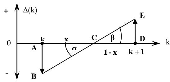 Figure 3: Simplification scheme for calculating DPP Panel label: Segment. $AB = |\Delta(\mathbf{k})|$, segment$ED = \Delta(\mathbf{k})$, the simplification is that the change$\Delta(\mathbf{k})$on the segment$AD$is represented by a straight line$BE$. Then at point$C$there comes a moment when equality(5)is satisfied and, since$D\alpha = D\beta$in triangles$\triangle ABC$and$VCDE$, it obviously follows $$ \frac {\mathrm {A B}}{\mathrm {A C}} = \frac {\mathrm {E D}}{\mathrm {C D}}. \tag {6} $$ A single segment AD can be represented as a sum $\mathrm{AD} = \mathrm{AC} + \mathrm{CD}$ or $\mathrm{AD} = \mathrm{x} + (1 - \mathrm{x})$, where $\mathbf{x}$ is the desired part of the year, which determines the payback moment, taking into account discounting, then from (6) $\frac{\left|\Delta(\mathbf{k})\right|}{\mathbf{x}} = \frac{\Delta(\mathbf{k} + 1)}{1 - \mathbf{x}}$ it is possible to determine the desired part of the year: $\mathbf{x} = \frac{\left|\Delta(\mathbf{k})\right|}{\left|\Delta(\mathbf{k})\right| + \Delta(\mathbf{k} + 1)}$. Thus, the result of the algorithm is the calculation of the discounted payback period according to the rule: $$ DPP\left(\mathbf{D}_t,\mathbf{I}_t,\mathrm{i},\mathrm{t}\right) = \mathbf{n}_1\Delta\mathrm{DPP} $$ where $\mathbf{n}_1$ is the duration of the investment part of the project, $\mathbf{D}_t$ and $\mathbf{I}_t$ are the sizes of investment and income payments, respectively, i - is the investor's rate of return, moreover, $\Delta \mathrm{DPP} = \mathrm{x}$ is calculated using a recursive-logical procedure: $$ \left\{ \begin{array}{l} \Delta D P P = k + \frac {\left| P _ {n _ {1}} ^ {(k)} - S _ {n _ {1}} \right|}{\left(P _ {n _ {1}} ^ {(k + 1)} - S _ {n _ {1}}\right) + \left| P _ {n _ {1}} ^ {(k)} - S _ {n _ {1}} \right|}, \\P _ {n _ {1}} ^ {(k)} < S _ {n _ {1}} < P _ {n _ {1}} ^ {(k + 1)} \end{array} \right. \tag{8} $$ $\mathbf{S}_{\mathrm{n_l}} = \sum_{t = 1}^{\mathrm{n_l}}\mathbf{x}_t\cdot (1 + \mathbf{i})^{\mathrm{n_l}\cdot t} -$ reduced to the point the accumulated amount of investment payments of the project; $\mathbf{P}_{\mathrm{n}_1}^{(\mathrm{k})} = \sum_{\mathrm{t} = \mathrm{n}_1 + 1}^{\mathrm{n}_1 + \mathrm{k}}\frac{\mathbf{y}_\mathrm{t}}{(1 + \mathrm{i})^{\mathrm{t}\cdot \mathrm{n}_1}} -$ the present value of the project revenue reduced to the point $t = n_{1}$ duration $\mathbf{n}_1 + \mathbf{k}$ $(k = 1,2\dots)$. $\mathbf{P}_{\mathrm{n_i}}^{(k + 1)} = \sum_{t = n_i + 1}^{n_i + k + 1}\frac{\mathbf{y}_t}{(1 + \mathrm{i})^{t\cdot n_i}} -$ the present value of the project revenue reduced to the point $t = n_1$ duration $\mathbf{n}_1 + \mathbf{k} + 1$ $(k = 1,2\dots)$ From (7) and (8) it follows that the calculation $\triangle DPP$ is a process of $k + 1$ successive steps, in each of which it is necessary to calculate the value $\mathbf{P}_{\mathrm{n}_1}^{(\mathrm{k})}$ and compare it with the value $\mathbf{S}_{\mathrm{n}_1}$ until the relation $\mathbf{P}_{\mathrm{n}_1}^{(\mathrm{k})} < \mathbf{S}_{\mathrm{n}_1} < \mathbf{P}_{\mathrm{n}_1}^{(\mathrm{k} + 1)}$ is reached. Only after that it is possible to calculate $\triangle DPP$ by the procedure (8), and then DPP by the rule (7). Of course, the computational complexity of such an algorithm may turn out to be quite high due to the uncertainty of the number of iterations required to implement procedure (8). In order to present the ratio for calculating DPP in an analytical form, it is necessary to use a technique, the idea of which is to replace the discrete flow of income payments with a financially equivalent continuous flow of the income part of the investment project, since the analysis of procedure (8) shows that the smaller the difference $\mathbf{P}_{\mathfrak{n}_1}^{(k + 1)} - \mathbf{P}_{\mathfrak{n}_1}^{(k)}$, the more accurately it is possible to determine $\triangle$ DPP and, respectively, DPP. 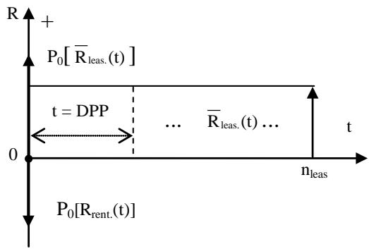In the scheme under consideration for the lessor (see Fig. 2), the financially equivalent flow of continuous lease payments is reflected in the scheme in Figure 4.  Figure 4: Financially equivalent continuous payment flow The present value of the project income stream with continuous payments $\overline{\mathbf{R}}_{\mathrm{leas.}}(t)$ and annual interest at rate $r_{\mathrm{leas.}}$ in accordance with the rules of financial mathematics will be determined as $$ \mathrm{P} _ {0} \left[ \overline{{\mathrm{R}}} _ {\text{leas}, \Pi \Pi_ {3.}} (\mathrm{t}) \right] = \overline{{\mathrm{R}}} \quad (\mathrm{t}) \cdot \frac{1 - \left(1 + \mathrm{r} _ {\text{leas}}\right) ^ {- \mathrm{n} _ {\text{leas}}}}{\ln \left(1 + \mathrm{r} _ {\text{leas}}\right)}. $$ The financial equivalence of such a flow with the flow of discrete payments $\overline{\mathbf{R}}_{\mathrm{leas.}}(t)$ will be ensured if the quality $\mathbf{P}_0\left[\mathbf{R}_{\mathrm{leas}}(t)\right] = \sum_{t = n_1}^{n_{\mathrm{mrs}}} \frac{\mathbf{R}_{\mathrm{leas}}(t)}{(1 + \mathbf{r}_{\mathrm{leas}})^t} = \mathbf{P}_0\left[\overline{\mathbf{R}}_{\mathrm{leas}}(t)\right]$ is fulfilled, whence it follows $$ \overline{\mathrm{R}}_{\mathrm{лиз.}}(t) = \frac{\ln(1 + \mathrm{r}_{\mathrm{leas}})}{1 - (1 + \mathrm{r}_{\mathrm{leas}})^{-\mathrm{n}_{\mathrm{лиз.}}}} \cdot \sum_{t = n_1}^{\mathrm{n}_{\mathrm{лиз.}}} \frac{\mathrm{R}_{\mathrm{leas}}(t)}{(1 + \mathrm{r}_{\mathrm{leas}})^t} $$ According to the economic meaning of the discounted payback period, the present value of a continuous flow of income (leasing) payments with a duration of DPP should be equal to the present value of the entire flow of investment (lease) payments. Then $$ \mathrm{P} _ {0} \left[ \mathrm{R} _ {\text{leas}} (\mathrm{t}) \right] = \mathrm{P} _ {0} \left[ \overline{{\mathrm{R}}} _ {\text{leas}} (\mathrm{t}) \right] \Bigg | _ {\mathrm{t} = \mathrm{D P P}} = \overline{{\mathrm{R}}} _ {\text{leas}} (\mathrm{t}) \cdot \frac{1 - (1 + \mathrm{r} _ {\text{leas}}) ^ {- \mathrm{D P P}}}{\ln (1 + \mathrm{r} _ {\text{leas}})} \tag{10} $$ Taking into account here (9) and simple algebraic transformations, we obtain $$ \begin{array}{l} \mathrm{P}_{0} \left[ \overline{\mathrm{R}}_{\text{ЛИЗ.}} (\mathrm{t}) \right] \right|_{\mathrm{t = D P P}} = \frac{1 - \left(1 + \mathrm{r}_{\text{ЛИЗ.}}\right)^{-\mathrm{D P P}}}{1 - \left(1 + \mathrm{r}_{\text{ЛИЗ.}}\right)^{-\mathrm{n}_{\text{ЛИЗ.}}}} \cdot \sum_{\mathrm{t = 0}}^{\mathrm{n}_{\text{ЛИЗ.}}} \frac{\mathrm{R}_{\text{ЛИЗ.}} (\mathrm{t})}{\left(1 + \mathrm{r}_{\text{ЛИЗ.}}\right)^{\mathrm{t}}} = \\= \frac{1 - \left(1 + \mathrm{r}_{\mathrm{ЛИЗ.}}\right)^{-\mathrm{D P P}}}{1 - \left(1 + \mathrm{r}_{\mathrm{ЛИЗ.}}\right)^{-\mathrm{n}_{\mathrm{ЛИЗ.}}}} \cdot \mathrm{P}_{0\text{ЛИЗ.}} [ \mathrm{R} (\mathrm{t}) ]. \tag{11} \\end{array} $$ Using the results (11) in relation (10), we obtain the equation $$ \mathrm{P} _ {0} \left[ \mathrm{R} _ {\text{leas}} (\mathrm{t}) \right] = \frac{1 - \left(1 + \mathrm{r} _ {\text{leas}} ^ {\mathrm{D P P}}\right)}{1 - \left(1 + \mathrm{r} _ {\text{leas}}\right) ^ {- \mathrm{n} _ {\text{leas}}}} \cdot \mathrm{P} _ {0} \left[ \mathrm{R} _ {\text{rent}} (\mathrm{t}) \right], \tag{11a} $$ solving which with respect to DPP, after the appropriate transformations and logarithm, we obtain the final result $$ \mathrm{DPP} = - \frac{\ln \left\{1 - \frac{\mathrm{P}_{0\mathrm{a}2}[\mathrm{R}(\mathrm{t})]}{\mathrm{P}_{0\mathrm{a}3.}[\mathrm{R}(\mathrm{t})]} \cdot \left[ 1 - \left(1 + \mathrm{r}_{\mathrm{JH3.}}\right)^{-\mathrm{n}_{\mathrm{JH3.}}} \right] \right\}}{\ln \left(1 + \mathrm{r}_{\mathrm{JH3.}}\right)}. \tag{12} $$ The minus sign in (12) means that the DPP value will be positive if the value of the logarithm is negative, i.e. the argument of the logarithm is less than 1. This means that the critical payback condition for this operation is, in principle, determined by the relation: $$ \frac{\mathrm{P} _ {0} \left[ \mathrm{R} _ {\text{rent}} (\mathrm{t}) \right]}{\mathrm{P} _ {0} \left[ \mathrm{R} _ {\text{leas}} (\mathrm{t}) \right]} \cdot \left[ 1 - \left(1 + \mathrm{r} _ {\text{leas}}\right) ^ {- \mathrm{n} _ {\text{leas}}} \right] = 1, \tag{13} $$ in which income payments from equipment leasing can only be repaid by interest on equipment rental from the manufacturer, but the principal debt (equipment cost) will never be repaid (perpetual rent). If $$ \frac{\mathrm{P} _ {0} \left[ \mathrm{R} _ {\text{rent}} (\mathrm{t}) \right]}{\mathrm{P} _ {0} \left[ \mathrm{R} _ {\text{leas}} (\mathrm{t}) \right]} \cdot \left[ 1 - \left(1 + \mathrm{r} _ {\text{leas}}\right) ^ {- \mathrm{n} _ {\text{leas}}} \right] < 1 $$ negative outflows of lease payments to the manufacturer will be "covered" by positive inflows of lease payments from the lessee so that the project pays off and NPV > 0. If $$ \frac{\mathrm{P} _ {0} \left[ \mathrm{R} _ {\text{rent}} (\mathrm{t}) \right]}{\mathrm{P} _ {0} \left[ \mathrm{R} _ {\text{leas}} (\mathrm{t}) \right]} \cdot \left[ 1 - \left(1 + \mathrm{r} _ {\text{leas}}\right) ^ {- \mathrm{n} _ {\text{leas}}} \right] > 1, $$ the main debt to the manufacturer with interest on the lease will not only not be repaid, but will also increase. In addition, expression (12) allows us to draw an important practical conclusion when analyzing the effectiveness of a leasing operation: if DPP = n leas, then $\frac{\mathrm{P_0}[\mathrm{R_{leas}}(t)]}{\mathrm{P_0}[\mathrm{R_{rent}}(t)]} = 1$ therefore, based on (1) and (2) in this case, NPV = 0, and DPI = 1. This follows from the passage to the limit in expression (12); if denoted $\frac{\mathrm{P_0}[\mathrm{R_{leas}}(t)]}{\mathrm{P_0}[\mathrm{R_{rent}}(t)]} = \mathrm{A}$, then $$ \begin{array}{l} \lim _ {\mathrm {A} \rightarrow \mathbf {1}} \mathrm {D P P} (\mathrm {A}) = \lim _ {\mathrm {A} \rightarrow \mathbf {1}} \left\{- \frac {\ln \left\{1 - \mathrm {A} \cdot \left[ 1 - \left(1 + \mathrm {r} _ {\mathrm {I H 3}}\right) ^ {- n _ {\mathrm {I H 3}}} \right]\right\}}{\ln (1 + \mathrm {r} _ {\mathrm {I H 3}})} \right\} = \\= \lim _ {A \rightarrow I} \left\{- \frac {\ln \left(1 + r _ {I H 3}\right) ^ {- n _ {I H 3}}}{\ln \left(1 + r _ {I H 3}\right)} \right\} = \lim _ {A \rightarrow I} \left\{- \cdot \left(- n _ {I H 3}\right) \frac {\ln \left(1 + r _ {I H 3}\right)}{\ln \left(1 + r _ {I H 3}\right)} \right\} = n _ {I H 3}. \\\end{array} $$ The results obtained actually determine the range of payback period values, which will allow us to draw conclusions regarding the economic efficiency of the leasing operation as an investment project for the lessor: $$ 0 < \mathrm{DPP} < \left(\mathrm{DPP}_{\text{crit}} = n_{\mathrm{leas}}\right) $$ Thus, comparing the DPP value obtained using the analytical expression (12) with a given value $\mathbf{n}_{\mathrm{leas}}$, one can determine the economic efficiency of this operation: if DPP $> \mathbf{n}_{\mathrm{leas}}$, then the operation is unprofitable for the lessor (NPV $< 0$ ), if DPP $< \mathbf{n}_{\mathrm{leas}}$ - the operation brings net income (NPV $> 0$ ). All of the above also allows us to conclude that the DPP indicator of the discounted payback period of a leasing operation for a lessor as a type of investment project based on the analytical expression (12) can be an alternative indicator of the operation's efficiency along with NPV and DPI. As an illustration of the results obtained, Fig. Figure 5 shows the dependency graph $\mathbf{DPP} = \mathbf{f}\left(\mathbf{R}_{\mathrm{leas}}\right)$ according to formula (12) based on the following data: types of rental and income payment flows - annual annuities postnumerando, $\mathbf{R}_{\mathrm{rent}} = 10$ thousand rubles, $$ n_{\mathrm{rent}} = 6\text{years}, r_{\mathrm{rent}} = 10\%, n_{\mathrm{leas}} = 7\text{years}, r_{\mathrm{leas}} = 10\%. $$ 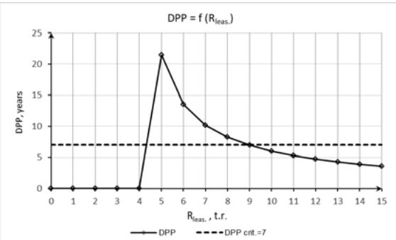 Figure 7: Limit value calculation r $\mathbf{r}_{\mathrm{leas}}^{\mathrm{crit}}$ Figure 5: The dependence of the payback period on the amount of lease payments Quantitatively, the limiting value $\mathbf{R}_{\mathrm{leas}}$, which determines the loss margin, is found by solving the nonlinear equation $$ DPP = - \frac{\ln \left\{1 - \frac{P _ {0} \left[ R _ {\text{rent}} (t) \right]}{P _ {0} \left[ R _ {\text{leas}} (t) \right]} \cdot \left[ 1 - \left(1 + r _ {\text{leas}}\right) ^ {- n _ {\text{leas}}} \right] \right\}}{\ln \left(1 + r _ {\text{leas}}\right)} = n _ {\text{leas}} $$ relatively $\mathbf{R}_{\mathrm{leas}}$ using the MS Excel module "Parameter selection". For example, using the above example data to plot the graph in Figure 5, you can get the limit value $\mathbf{R}_{\mathrm{leas}}^{\mathrm{crit}}$, which determines the loss margin of the leasing operation for the lessor. As shown in Figure 6 value $\mathbf{R}_{\mathrm{leas}}^{\mathrm{crit}} \approx 8.95$. R_{\mathrm{leas}} = 8,945999 <table><tr><td>B</td><td>C</td><td>D</td><td>E</td><td>F</td><td>G</td></tr><tr><td></td><td></td><td></td><td></td><td></td><td></td></tr><tr><td>Rrent =</td><td>r rent</td><td>n rent</td><td>Rleas =</td><td>r leas</td><td>n leas</td></tr><tr><td>10</td><td>0,1</td><td>6</td><td>8,945999</td><td>0,1</td><td>7</td></tr><tr><td></td><td></td><td></td><td></td><td></td><td></td></tr><tr><td>P0[Rrent] =</td><td>43,55261</td><td></td><td>P0[Rleas] =</td><td>43,55287</td><td></td></tr><tr><td></td><td></td><td></td><td></td><td></td><td></td></tr><tr><td>DPP =</td><td>6,999939</td><td></td><td></td><td></td><td></td></tr></table> Figure 6: Limit value calculation $\mathbf{R}_{\mathrm{leas}}^{\mathrm{crit}}$ Similarly, the solution of the non-linear equation (16) will allow us to determine the limit value of the rate $r_{\text{leas}}^{\text{crit}}$, which determines the loss margin, is the leasing operation for the lessor. For example, using the above example data to plot the graph in Figure 5, you can get the limit value of the rate $r_{\text{leas}}^{\text{crit}}$, which determines the loss margin of the leasing operation for the lessor. As shown in Figure 7 value $r_{\text{leas}}^{\text{crit}} \approx 0.135$. R_{\text{rent}} = r_{\text{rent}} \quad n_{\text{rent}} \quad R_{\text{leas}} = r_{\text{leas}} \quad n_{\text{leas}} \quad 10 \quad 0,1 \quad 6 \quad 10 \quad 0,134938 \quad 7 \quad P_{0}[R_{\text{rent}}] = 43,55261 \quad P_{0}[R_{\text{leas}}] = 43,55457 \quad DPP = 6,999494 <table><tr><td>Rrent =</td><td>rrent</td><td>nrent</td><td>Rleas =</td><td>rleas</td><td>nleas</td></tr><tr><td>10</td><td>0,1</td><td>6</td><td>10</td><td>0,134938</td><td>7</td></tr><tr><td>P0[Rrent] =</td><td>43,55261</td><td></td><td>P0[Rleas] =</td><td>43,55457</td><td></td></tr><tr><td>DPP =</td><td>6,999494</td><td></td><td></td><td></td><td></td></tr></table> The results obtained and the conclusions drawn are confirmed by the graph in Figure 8 and the graph in fig. 9, which are built on the basis of the numerical data of the example used above to plot the graph in Figure 5.  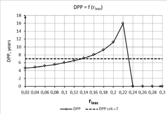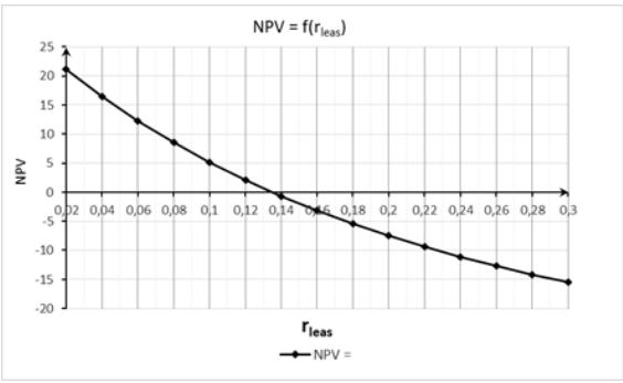 Figure 8: The dependence of DPP on the rate $\mathbf{r}_{\mathrm{leas}}$ Figure 9: The dependence of NPV on the rate $\mathbf{r}_{\mathrm{leas}}$ Data analysis in Figure 8 and 9 shows that the value $r_{\text{leas}}^{\text{crit}} \approx 0.135$ obtained by solving equation (16) corresponds to the IRR of the investment project with the numerical example data selected for plotting in Figure 5. This circumstance once again confirms the conclusion that the DPP indicator of the discounted payback period of a leasing operation for a lessor as a type of investment project based on the analytical expression (12) can be an alternative indicator of the operation efficiency along with NPV and DPI. The assessment of the effectiveness of leasing for the lessor in the case of purchasing equipment from the manufacturer at the expense of the EC will obviously be determined by the same ratios as in the case of leasing, since the financial and time scheme for implementation will be similar to the scheme in Figure 2. The only difference will be that the $\%$ rate $r_{\text{rent}}$ on the lease is replaced by the $\%$ rate $r_{\text{purch}}$ on the purchase in installments, and the amount of the lease payment $R_{\text{rent}}$ is replaced by the amount of the payment upon purchase $-R_{\text{purch}}$. Consequently, all indicators and conditions for the effectiveness of the leasing operation for the lessor (12) - (15) will also be valid in the case of purchasing equipment from the manufacturer with appropriate replacements. This article provides an analysis of the effectiveness of only the first option for implementing a leasing operation for a lessor out of the four that were considered in the general scheme in Figure 1. In addition, the first version of the general scheme can be supplemented with the case when the leased equipment after the lease period has a certain residual value (which in this article is considered equal to zero). Then, of course, the economic and mathematical analysis will be more difficult, but the author hopes to consider it and other options for the general scheme for implementing the leasing operation for the lessor in his subsequent articles. ## IV. CONCLUSIONS The approach used in this article to the analysis of leasing as an investment project makes it possible to use the indicators of the reduced net income and the profitability index for the analytical evaluation of the effectiveness of leasing operations. In addition, the author's method for obtaining the analytical formula for the discounted payback period of the project allows us to significantly expand the analysis of the effectiveness of dynamic operations in the economy, both in terms of mathematical rigor and in terms of graphic clarity. The results obtained make it possible to obtain specific mathematical conditions that link the parameters of leasing operations, the implementation of which will be economically beneficial for the lessor as a necessary financial and economic link in the modern economy. In addition, the obtained analytical expressions for performance indicators are functions of the same variables, which will undoubtedly allow them to be used to solve the problem of finding not only an operational, but also optimal solution under given conditions from the point of view of the selected criterion.

Generating HTML Viewer...

References

17 Cites in Article
C Drury,S Braund (1990). Unknown Title.
Arun Upneja,Raymond Schmidgall (2001). An Investigation of Leasing Practices in the U.S. Hotel Industry.
Alan Goodacre (2003). Operating lease finance in the UK retail sector.
Jean Shaoul (2007). Leasing Passenger Trains: The British Experience.
V Gazman (2011). Paper.
V Gazman (2013). The Impact of Alternative Models of Leasing on Financing Investments.
Veronica Vecchi,Mark Hellowell (2013). Leasing by public authorities in Italy: creating economic value from a balance sheet illusion.
Ngan Chau,Steven Schulz (2014). Selling Versus Leasing of Durable Goods: The Impact on Marketing Channels.
D Bülbül,F Noth,M Tyrell (2014). Unknown Title.
V Gazman (2017). Paper.
Vera Gerasimova (2018). Role of leasing for sustainable development of the Russian economy.
Na Zhang (2018). Leasing, legal environments, and growth: evidence from 76 countries.
Viktor Gazman (2019). Socio-economic Efficiency of the Leasing in Renewable Energy.
Jamila Leontieva,Ludmila Tarasova,Yulia Boiko,Eugenia Zaugarova (2019). Financing of investment activities of Russian energy enterprises.
A Podgornaya,T Abitov (2019). An Experimental Examination of Mobile Cloud Computing and IOT: Application, Techniques and Issues.
Patricia Van Loon,Charles Delagarde,Luk Van Wassenhove,Aleš Mihelič (2020). Leasing or buying white goods: comparing manufacturer profitability versus cost to consumer.
Tatiana Litvinova (2020). Agricultural Lease as a Perspective Mechanism of Development of Infrastructure of Entrepreneurship in the Agricultural Machinery Market.
No ethics committee approval was required for this article type.
Data Availability
Not applicable for this article.
How to Cite This Article
Yuri V Kirillov. 2026. \u201cEconomic and Mathematical Analysis of Leasing Efficiency Evaluation for a Lessor\u201d. Global Journal of Management and Business Research - C: Finance GJMBR-C Volume 24 (GJMBR Volume 24 Issue C2): .
Explore published articles in an immersive Augmented Reality environment. Our platform converts research papers into interactive 3D books, allowing readers to view and interact with content using AR and VR compatible devices.
Your published article is automatically converted into a realistic 3D book. Flip through pages and read research papers in a more engaging and interactive format.
The article examines the analysis of the conditions under which the economic activity of a leasing company, as a necessary link in the current crisis between manufacturers of modern equipment and enterprises operating on the market using it, is cost-effective. Since the lessor can simultaneously act both as a lessee or buyer of equipment from the manufacturer, on the one hand, and as a lessor of this equipment for the user enterprise, on the other hand, the analysis of the effectiveness of its activities was carried out in the form of an assessment of the effectiveness of financial inflows and outflows of the lessee and the lessor. An economic and mathematical analysis of the reduced net income of the lessor was carried out for four options for such a project: two options when the lessor acts as a tenant and a lessor, as well as a buyer and a lessor when using equity capital, and two similar options when using a loan. Analytical indicators of project effectiveness -reduced net income and profitability index -are supplemented by the payback period indicator, for the calculation of which, in practice, a laborious recursive-logical procedure is used. To obtain an analytical expression for the payback period, an original technique was used based on the replacement of a discrete stream of payments with a financially equivalent continuous stream.
Our website is actively being updated, and changes may occur frequently. Please clear your browser cache if needed. For feedback or error reporting, please email [email protected]
Thank you for connecting with us. We will respond to you shortly.