I. INTRODUCTION
In the concept of scalar-vector potential it is possible to isolate, at least, three cases of determining the tension of the electric field, which characterize actually the different versions of this concept [1-7].
a) Nonpotential electric field
If speech goes about the electric field of the single charge then its electric field will be determined by the relationship:
where - the projection on the direction
of the vector of the unit vector , of collinear to the vector ;
– the projection of the unit vector
, of collinear to vector , on the direction of normal to the vector , of that lying at one plane s .
Let us fix certain moment of time. Let us select the system of rectangular Cartesian space coordinates OXYZ so that at this moment the time the origin of coordinates would coincide with the moving point charge e, axis OX would be directed posigrade of charge v, and vector r it would lie in the plane XOY. Then vector r can be assigned by two coordinates x, also, y along the axes OX and OY respectively. In this case longitudinal (along the axis OX) and transverse (along the axis OY) of the component of the vector of the tension of electric field at point r they will be equal respectively
Integration of these components for the appropriate coordinates gives:
where and – integration constant.
With the electric field proves to be potential with the known potential
but with the potentiality of field it is disrupted, i.e., there does not exist this function of potential, through which it would be possible to express the field strength according to the formula
Therefore such electric field of the moving charge must be examined as the superposition
longitudinal electric field with the potential (let us name its longitudinal potential)
and transverse electric field with the potential (let us name its transverse potential)
the fields having nontrivial components only on OX and OY:
Therefore in this case it is more correct to speak not about the concept of the scalar potential of charge, which depends on the speed, but about the concept of invariant longitudinal scalar potential and transverse scalar potential depending on the speed.
b) Potential electric field of Mende
Let us fix certain moment of time. Let us select the system of rectangular Cartesian space coordinates OXYZ so that at this moment the time the origin of coordinates would coincide with the moving point charge e, axis OY would be directed posigrade of charge v, and vector r, directed from one point of the concentration of charge to the next, at which the field is determined, it lay in the plane XOY. Then vector r can be assigned by two coordinates x, also, y along the axes OX and OY respectively.
Let us assume that electric field is the potential field, given by the scalar potential
where – the radius-vector of the point, at which is determined the field; – the distance between the charge and the point, at which is determined the field; – the component of charge rate e, is normal k r. Let there be x > 0, y > 0, then:
The strength of this field has transverse , which they are determined from the component and longitudinal component formulas:
c) Potential electric field with the transversely deformed scalar potential
Let us select the system of rectangular Cartesian space coordinates in the manner that in the case 2. The electrostatic potential of charge takes the form:
where - the radius-vector of the point, at which is determined the field; - the distance between the charge and this point.
Let us assume that the dynamic potential of charge is the transversely deformed electrostatic potential. Then we obtain the potential electric field, described by the scalar potential,
where – the module of charge rate, moreover .
Taking into account expression for the electrostatic potential, we obtain formula for the dynamic potential:
The transverse and longitudinal components of the field strength will be written down in the form
With , y = 0 we have:
With , we have:
d) Conclusions of three cases examined are the following
Thus, three versions of the determination of electrical pour on in the concept of the scalar-vector potential proposed:
- the nonpotential field, whose longitudinal component of tension does not depend on speed, but transverse – depends;
2. potential field in Mende's version;
- potential field with the transversely deformed scalar potential.
Last two versions characterize the potential field, in which in general case both components depend on speed; however, for this field it is possible to isolate two extreme special cases for the points, at which this field is determined: if to point (at the coordinate system proposed these points lie on the axis the transverse component ) of field it is absent into some, then longitudinal does not depend on speed; if to point (at the coordinate system proposed these points lie on the axis the longitudinal component ) of field it is absent into some, then transverse depends on speed by the simple dependence, which is obtained by the multiplication of the corresponding strength of electrostatic field to the coefficient .
The potentiality of electric field means that during the motion in this field of trial charge along the locked trajectory the work is not accomplished. But if scalar potential changes in the time, then in the time changes electric field the, as a result of which this property of the absence of the perfect work, strictly speaking, it is not carried out. However, in this case for each assigned moment of time potential electric field (last two versions) can be defined as the undertaken with the opposite sign gradient of scalar potential.
An important difference in the first and third versions in the first version lies in the fact that occurs the lateral deformation of the strength of the field (it it leads to the nonpotentiality of field), and in the third – the lateral deformation the scalar potential field (it it leads to the dependence on the speed in general case of both components of the field strength).
In the present monograph the basis is undertaken the second version of concept, although the third version from a physical point of view is presented to us not less, but, possibly, by more promising, and the first version is also is sufficiently promising. In connection with this, one of the most important tasks of further studies – the determination of version, most adequate of reality.
II. LAWS OF THE ELECTRO-ELECTRICAL INDUCTION
We will consider that the charge e accomplishes fluctuating motion along the axis y, in the environment of the origin of coordinates 0 (Fig. 13), moreover the amplitude of the fluctuations of charge is considerably lower than the distance from the charge to the observed point. According to the second version of concept, the scalar potential of charge at point with the abscissa x and the ordinate y = 0 (fixed point (1) in Fig. 1) depends on the component of its velocity, normal to the vector , connecting observation point and the moving charge:
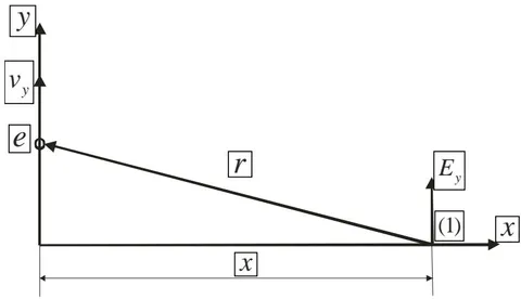
According to relationship , the projection on the axis y of the tension of the induced electric field at the same point is equal
Counting in view of the smallness of the amplitude of fluctuations radius-vector by constant, let us rewrite last equality in the form:
a) Taking into account that
we obtain from (2.2):
Counting the charge rate of much smaller speed of light and taking only first term of expansion , from (2.3) we have:
where - acceleration of charge.
If we as the direction of emission take the vector, which lies at the plane xy, and which constitutes with the axis y the angle , then relationship (2.4) takes the form:
This relationship determines the radiation pattern of shaping of the induced electric field.
Let us introduce delay in the scalar-vector potential, considering as its conditioned propagation of field in this medium with the speed of light:
where - component of the charge rate e, normal to the vector r at the moment of the time , r - distance between the charge and the point, at which t.
Again using a relationship , let us find field at the same point:
Considering again radius-vector constant, we will obtain:
b) Taking into account that
From (2.6) we obtain the complete emission law of the moving charge:
Counting the charge rate of much smaller speed of light and taking only first term of expansion , from (2.7) we will obtain the wave equation, which defines both the amplitude, and phase response of the wave of electric field, radiated by the moving charge:
where - being late acceleration of charge.
After selecting by the direction of emission vector in the plane xy, component with the axis y angle , from (2.8) we will obtain the relationship, which determines known radiation pattern of dipole source (complete diagram it is symmetrical relative to the axis y):
Known in the electrodynamics being late vector potential
it is here introduced not heuristic and phenomenologically, but on the basis of the being late scalar-vector potential. In Maxwell equations the electric fields of wave are vortex, while in this concept – are gradient.
Still one possibility of relationship (2.9) – the description of the dipole emission of electromagnetic waves by the charges, which are varied in the electric field. Time derivative of the dipole moment (vector d it is directed from the negative charge toward the positive)
it is connected with the current:
The substitution of last equality for a in (2.9) gives the known [8] emission law of the being varied dipole
Thus, the field of the being varied electric dipole is determined by the superposition of electrical induction pour on the emissions (2.8), (2.9), (2.11), of those connected with the acceleration of charge, and electrical pour on static dipole, that are changed according to dependence on the time of the distance between the charges. The process of emission is connected with the transformation of energy pour on static dipole into the energy pour on emissions.
Laws (2.8), (2.9), (2.11) do not use magnetic fields and vector potentials, showing thus the fundamentality of electrical and the second-rateness of magnetic pour on.
Relationship (2.9) makes it possible to obtain the laws of reflection and scattering of electrical pour on by the totality of the charges, set to the forced motion by external (strange) electric field. The superposition of electrical pour on, radiated by all charges, it is electrical wave.
The acceleration of charge under the action of strange electric field is equal
Taking into account this relationship (18.9) assumes the form
where the determining ability of charge to re-emit external field the value
Let us name the coefficient of scattering (re-emission) charge in the assigned direction.
The current wave of the displacement accompanies the wave of electric field:
If charge accomplishes its motion under the action of the electric field , then bias current in the distant zone will be written down as
The wave of electric field (18.12) and laggard behind it on the current wave of displacement (2.13) form the wave that named there electric current.
In parallel with the electrical waves it is possible to introduce magnetic waves, if we assume that
Such magnetic field - is vortex. Comparing (2.13) and (2.14) we obtain:
Integrating this relationship on the coordinate, we find the value of the magnetic field
Thus, relationship (2.12), (2.13) and (2.15) can be named the laws of electrical induction, since, they give the direct coupling between the electric fields, applied to the charge, and by fields and by currents induced by this charge in its environment. Charge itself comes out [v] in the role of the transformer, which ensures this reradiation. Magnetic field (2.15) is directed normally both toward the electric field and toward the direction of propagation. In this case it is executed:
where Z - wave drag of free space.
Wave drag determines the active power of losses on the single area, located normal to the direction of propagation of the wave:
This relationship determines the power flux of the electric current wave through this area according to Poynting theorem.
Thus, any wave process in the fields of electromagnetic nature is reduced to the electric current waves in the space, characterized by its wave drag. This examination does not require the attraction of the concepts of magnetic field and its vector potential. Nevertheless, these concepts can be additionally introduced, clearly dividing fields to the gradient (electrical) and the vortex (magnetic) according to Helmholtz's theorem, which says, that any single-valued and continuous vectorial field F, turning into zero at infinity, can be represented, and besides uniquely, in the form the sum of the gradient of a certain scalar function and rotor of a certain vector function C, divergence of which is equal to zero:
thus, the construction of electrodynamics should have been begun from the acknowledgement of the dependence of scalar potential on the speed. But nature very deeply hides its secrets, and in order to come to this simple conclusion, it was necessary to pass way by length almost into two centuries.
The grit, which so harmoniously were erected around the magnet poles, in a straight manner indicated the presence of some power pour on potential nature, but to this they did not turn attention; therefore it turned out that all examined only tip of the iceberg, whose substantial part remained invisible of almost two hundred years.
Is exponential quotation from[9]: «But in what does consist the basic initial reason for the discrepancy of the built by Maxwell electrodynamics? For a single-valued answer to this question... it should be noted that even in its time, Ampère, Gauss, Lenz, Neumann, Weber, Riemann and others stood on the point of view that, without being turned to the concept "of magnetic field", any magnetic interactions can be reduced to usual interactions of current elements or moving charges... In the electrodynamics possessed then the point of view of Faraday and Maxwell, that the electrical and "magnetic" fields are the independent physical essences, although connected together. In the prevailing then historical situation given, erroneous from a physical point of view, assumptions predetermined by themselves entire further motion of the development of electrodynamics with the deliberately placed into it insoluble contradictions and the paradoxes». And further there: «For the noncontradictory reflection of the physical essence of the laws of electromagnetism necessary to completely forego any concepts "magnetic field" as certain independent physical essence... for determining the forces of interaction of moving in the physical vacuum of real space electric charges completely sufficient to consider the deformation of electrical pour on these charges, caused by the trivial effects of the being late potentials... To there remains only be surprised at the sagacity of Ampère, which warned that if we in the electrodynamics do not forego ourselves the concept "magnet", then subsequently this threatens by incredible confusion in the theory.»
One should assume that the basis of the overwhelming majority of the static and dynamic phenomena of electrodynamics – the assuming dependence of the scalar potential of charge on the speed of its motion formula
or the analogous to it formula, which reflects the different version of the concept of the scalar-vector potential. From this formula it follows and static interaction of charges, and laws of power interaction in the case of their mutual motion, and emission laws and scattering. This approach made it possible to explain from the positions of classical electrodynamics such phenomena as phase aberration and the transverse Doppler effect, which within the framework the classical electrodynamics of explanation did not find. After entire aforesaid it is possible to remove construction forests, such as magnetic field and magnetic vector potential, which do not allow here already almost two hundred years to see the building of electrodynamics in entire its sublimity and beauty.
Let us point out that one of the fundamental equations of induction
could be obtained directly from the Ampere law, still long before appeared Maxwell equations. The Ampere law, expressed in the vector form, determines magnetic field at the point
where I - current in the element dl, r - vector, directed from dl to the point.
It is possible to show that
therefore finally we will obtain:
where
The remarkable property of this expression is that the vector potential depends from the distance to the observation point as 1/r. Specifically, this property makes it possible to obtain emission laws.
Since. , where - a charge of the unit of the length of conductor, from (2.16) we have:
For the single charge e this relationship takes the form:
Since
that in the general case we have (here a - the acceleration of charge):
and we will obtain for a special case of single charge:
If we in (2.17), (2.18) consider the propagation time delay of potentials and that the fact that for the vacuum , these equalities will take the form:
Relationships (2.19) (2.20) represent wave equations. Let us note that these equations - this solution of Maxwell' equations, but in this case they are obtained directly from the Ampere law, not at all coming running to Maxwell equations. To there remains only present the question, why electrodynamics in its time is not banal by this method?
Given examples show, as electrodynamics in the time of its existence little moved. The phenomenon of electromagnetic induction Faraday opened into 1831 and already almost 200 years its study underwent practically no changes, and the physical causes for the most elementary electrodynamic phenomena, until now, were misunderstood. Certainly, for his time Faraday was genius, but that they did make physics after it? Even such geniuses, as Maxwell and Hertz, did not establish fundamental role in the entire classical electrodynamics of the dependence of the scalar potential of charge on his relative speed. Subsequently such scientists as Nikolayev and Marinov their theoretical and experimental studies were conducted in this direction, but proper acknowledgement as scientific association these works so did not obtain.
III. CONCLUSION
All dynamic laws of electrodynamics, connected with the motion of charge, follow from the concept of scalar-vector potential. In the article it is shown that alsoz of this concept follow the emission laws. These laws are introduced with the aid of the being late scalar vector potential. This approach gives the possibility to understand physics of the process of emission and to obtain all necessary laws of this process.