## I. INTRODUCTION According to Chopra and Meindil 2011, supply chain is a system that consists of a manufacturer, suppliers, transporters, distributors and retailers; where they all share information and goods and services are delivered among them to meet up with the demand of consumers. Considering the set of entities involved, supply chain is considered as a major aspect in the business circle. It is a whole cycle of procedures and end-to-end flow of materials, information and funds starting from the product design stage to fulfilment. As noted by Casson 2013, economics factors are the key factor in supply chain as it shows greater impact on size and shape. Beyond economic factors, Ketchen and Giunipero 2004 highlighted the effect of strategic choices on supply chain set up, coordination and operation. To deliver best and optimal solution, supply chain activities must be strategically laid out, coordinated and handled. Proper coordination will emanate from balancing the demand and supply ends. Various variables such as weather, market trends, and season, consumer behaviour exist between the two ends and thus coordinate planning must be fashioned out. The volatility in these variables prompt for demand forecasting. As mentioned by Hope and Fraser 2003, demand forecasting is one of the prerequisites for strategical planning in supply chain management. Many techniques and methods have been used to investigate contributing variables and forecasting of orders based on historical data. In this study machine learning regressors will be used to make order predictions using dataset acquired on the field for 60 days in a Brazilian logistics company. Machine learning is a sophisticated methods posit by advancement in computing technology where historical data are trained to build models which are subsequently used to make predictions. It exists as classification or regression means. For regression, predictions are made for continuous variables like demand in supply chain. According to Al-Jarrah et al 2015, machine learning is perfectly efficient in the analysis of voluminous data that exist in demand forecasting study. To effect more accurate demand prediction, robust regressors models will be developed using Python Library PyCaretwhile key contributing features are validated through feature importance plot. The various machine learning models (Ridge, LASSO, XGBoost, Bayesian Ridge, Linear Regression, Gradient Boosting, KNN, Random Forest and others) will run concurrently and their prediction performance measured with Mean Absolute Error (MAE): the mean absolute differences between predicted values and actual demand values. The lesser the MAE, the better the model predictions. ## II. LITERATURE REVIEW One of the important steps in supply chain planning is demand forecasting. By standard forecasting includes element of uncertainty as it is often hard to predict perfectly in a consistent manner. Thus, because of volatility involved in demand and uncertainty in forecasting, many research have been carried out over the years to improve decision making in supply chain. Carbonneau, Laframboise and Vahidor 2008 classified naive method, average method, moving average and trend as traditional methods and viewed them as solution approach based on linear demand idealization. Due to emerging complexity in demand situations in supply chain field, non-linear techniques were proposed in their paper to handle the complexity. They made use of machine learning techniques-neural network, recurrent neural networks and SVM to predict future demand and confirmed better outcomes compared to the traditional methods. MAE was used to compute error analysis for their model predictors in order to evaluate which among them best fits the study dataset. The results revealed that recurrent neural networks and SVM yielded most accurate predictions. A similar investigation by Wang 2012 using large paper enterprise dataset showed that support vector regression produced excellent performance. A more comprehensive study is seen in the work of Rivera-Castro et al 2019 where their experiments was performed using thirteen techniques that cut across times series and machine learning (Adaboost, ARIMAX, ARIMA, Bayesian Structure Time Series (BSTS), Bayesian Structural Time Series with a Bayesian Classifier (BSTS Classifier), Ensemble of Gradient Boosting, Ridge Regression, Kernel Regression, LASSO, Neural Network, Poisson Regression, Random Forest and Support Vector Regression). Symmetric Mean Absolute Percent Error (SMAPE) was used to evaluate the model's performance and Adaboost yielded best model with SMAPE of 0.17 followed by ensemble of Random Forest 0.18. Review of literatures has shown paradigm shift from traditional approach (Historical Analogy, Scenario Planning, Moving Averages, Exponential Smoothing and others) of predicting demand to more sophisticated tools of statistical methods and machine learning. In order to improve existing knowledge on demand forecasting, this study will follow the path of Rivera-Castro et al 2019 by making using of advanced Python Library that yield prediction across many regressions' algorithms simultaneously. Pycaret is an open-source machine learning library and it is low-code. It is distinct in its ability to train and evaluate multiple models with few line of codes. Another improvement is mode of error analysis which is run through MAE, MSE, RMSE, RMSLE and MAPE for each of the models. Thus, there is opportunity for utilization of many metricsto gauge prediction performances. ## III. METHODOLOGY ### a) Data Pre-processing The dataset utilized for this investigation is from UCI repository Daily Demand Forecasting Orders - UCI Machine Learning Repository. It was acquired on the field by a Brazilian Logistic company for a period of sixty days. The attribute of the dataset was shown using Pandas library at pre-processing stage. 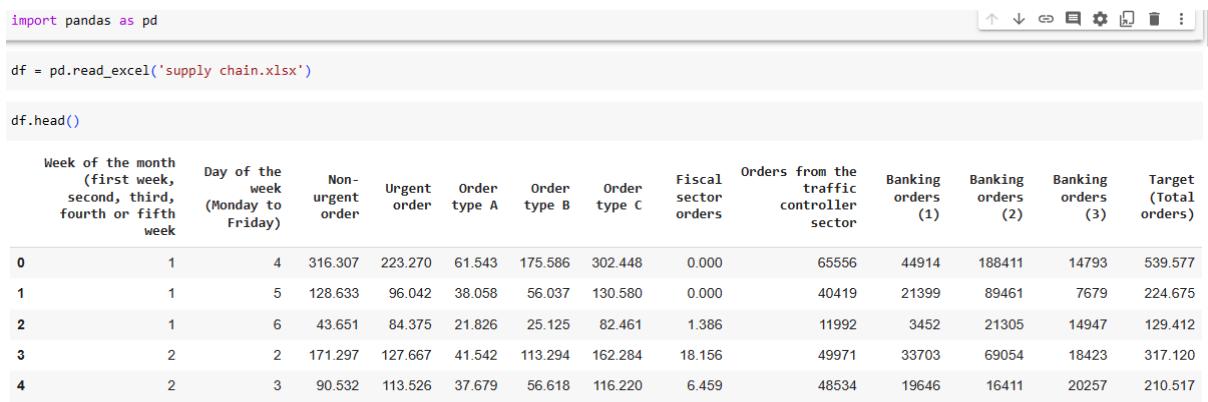 Figure 1: Importing Data using Pandas The dataset was validated for occurrence of missing values in the coding environment. 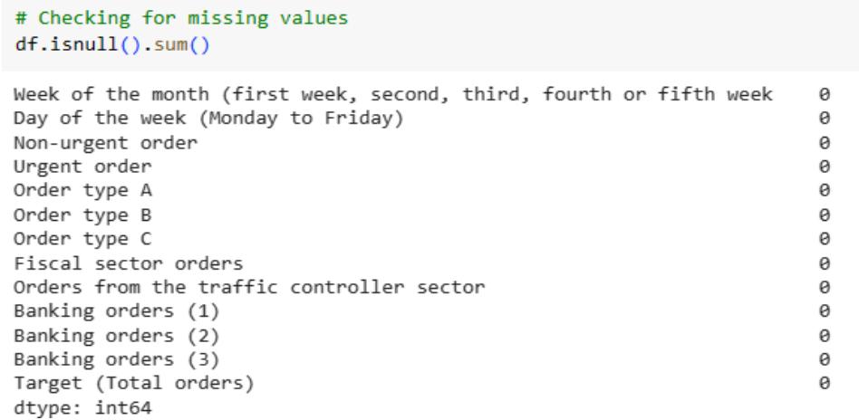 Figure 2: Checking for Missing Values Summary statistics of the dataset was evaluated to understand the distribution of the variables. This provides insights relevant to our analysis. <table><tr><td colspan="13"># Summary statisticsdf.describe()</td></tr><tr><td></td><td>Week of the month (first week, second, third, fourth or fifth week)</td><td>Day of the week (Monday to Friday)</td><td>Non-urgent order</td><td>Urgent order</td><td>Order type A</td><td>Order type B</td><td>Order type C</td><td>Fiscal sector orders</td><td>Orders from the traffic controller sector</td><td>Banking orders (1)</td><td>Banking orders (2)</td><td>Banking orders (3)</td></tr><tr><td>count</td><td>60.000000</td><td>60.000000</td><td>60.000000</td><td>60.000000</td><td>60.000000</td><td>60.000000</td><td>60.000000</td><td>60.000000</td><td>60.000000</td><td>60.000000</td><td>60.00000</td><td>6</td></tr><tr><td>mean</td><td>3.016667</td><td>4.033333</td><td>172.554933</td><td>118.920850</td><td>52.112217</td><td>109.229850</td><td>139.531250</td><td>77.396133</td><td>44504.350000</td><td>46640.833333</td><td>79401.483333</td><td>23114.633333</td></tr><tr><td>std</td><td>1.282102</td><td>1.401775</td><td>69.505788</td><td>27.170929</td><td>18.829911</td><td>50.741388</td><td>41.442932</td><td>186.502470</td><td>12197.905134</td><td>45220.736293</td><td>40504.420041</td><td>13148.039829</td></tr><tr><td>min</td><td>1.000000</td><td>2.000000</td><td>43.651000</td><td>77.371000</td><td>21.826000</td><td>25.125000</td><td>74.372000</td><td>0.000000</td><td>11992.000000</td><td>3452.000000</td><td>16411.000000</td><td>7679.000000</td></tr><tr><td>25%</td><td>2.000000</td><td>3.000000</td><td>125.348000</td><td>100.888000</td><td>39.456250</td><td>74.916250</td><td>113.632250</td><td>1.243250</td><td>34994.250000</td><td>20130.000000</td><td>50680.500000</td><td>23609.750000</td></tr><tr><td>50%</td><td>3.000000</td><td>4.000000</td><td>151.062500</td><td>113.114500</td><td>47.166500</td><td>99.482000</td><td>127.990000</td><td>7.831500</td><td>44312.000000</td><td>32527.500000</td><td>67181.000000</td><td>28181.500000</td></tr><tr><td>75%</td><td>4.000000</td><td>5.000000</td><td>194.606500</td><td>132.108250</td><td>58.463750</td><td>132.171000</td><td>160.107500</td><td>20.360750</td><td>52111.750000</td><td>45118.750000</td><td>94787.750000</td><td>31047.750000</td></tr><tr><td>max</td><td>5.000000</td><td>6.000000</td><td>435.304000</td><td>223.270000</td><td>118.178000</td><td>267.342000</td><td>302.448000</td><td>865.000000</td><td>71772.000000</td><td>210508.000000</td><td>188411.000000</td><td>617839.000000</td></tr></table> Figure 3: Summary Statistics for Dataset Attributes The average number of non-urgent orders is around 172.55, with a standard deviation of 69.50. The minimum number of non-urgent orders is 43.65, and the maximum is 435.30. The average number of urgent orders is around 118.92, with a standard deviation of 27.17. The minimum number of urgent orders is 77.37, and the maximum is 223.27. The average number of orders from the fiscal sector is around 77.39, with a standard deviation of 186.50. The minimum number of orders from the fiscal sector is 0, and the maximum is 865. The average number of orders from the traffic controller sector is around 44504.3, with a standard deviation of 12197.9. The minimum number of orders from the traffic controller sector is 11992, and the maximum is 71772. ### b) Exploratory Analysis To visualize the correlation between the dataset variables correlation matrix was employed. This will aid understanding of the relationships between different features and the target variable. The heatmap shows the correlation between different variables in the dataset. The colour scale represents the correlation coefficient, with dark blue indicating a strong negative correlation, light blue to light red indicating little to no correlation, and dark red indicating a strong positive correlation. 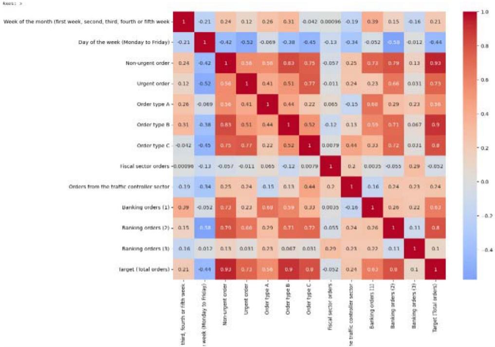 Figure 4: Heatmap to Show Correlation among Features From the heatmap, we can see that non-urgent order, urgent order, order type A, order type B, order type C, and orders from the traffic controller sector have a strong positive correlation with Target (Total orders). This suggests that these variables will be good predictors for the total orders. ### c) Machine Learning Predictions ## i. Linear Regression We started off from modelling weekly order volume with linear regression. Then make use of other regression models (Decision Tree and Random Forest) and compare their performances. The whole dataset is split into a training set and a test set in ratio 80:20. {"code_caption":[],"code_content":[{"type":"text","content":"from sklearn.model_selection import train_test_split\n# Defining the features and target variable\nx = df.drop('Target (Total orders)', axis=1)\ny = df['Target (Total orders)']\n# Splitting the data into training and test sets\nX_train, X_test, y_train, y_test = train_test_split(x, y, test_size=0.2, random_state=42) "}],"code_language":"python"} Figure 5: Splitting Dataset to Training and Test Sets Linear regression remits a linear relationship between the features and the target variable. The linear regressor is trained with training set while its performance is evaluated using the test set. 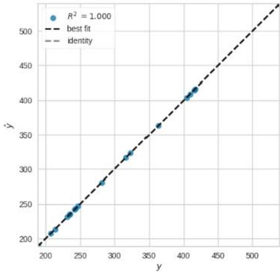{"algorithm_caption":[],"algorithm_content":[{"type":"text","content":"from sklearn.linear_model import LinearRegression \nfrom sklearn.metrics import mean_squared_error, r2_score \n# Creating a Linear Regression model \nlr "},{"type":"equation_inline","content":"="},{"type":"text","content":" LinearRegression() \n# Training the model \nlr.fit(x_train, y_train) \n# Making predictions on the test data \ny_pred_lr "},{"type":"equation_inline","content":"="},{"type":"text","content":" lr.predict(x_test) \n# Evaluating the model \nmse_lr "},{"type":"equation_inline","content":"="},{"type":"text","content":" mean_squared_error(y_test, y_pred_lr) \nr2_lr "},{"type":"equation_inline","content":"="},{"type":"text","content":" r2_score(y_test, y_pred_lr) \nmse_lr, r2_lr \n(4.668373655643919e-24, 1.0) "}]} Figure 6: Coding for Linear Regression 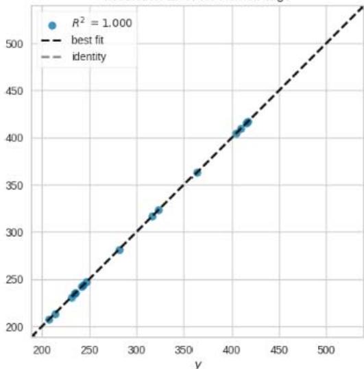The linear regression model has a Mean Squared Error (MSE) of approximately 4.24e-24 and an R-squared $(R^2)$ score of 1.0 on the test data. The $R^2$ score is a statistical measure that represents the proportion of the variance for a dependent variable that's explained by an independent variable(s) in a regression model. An $R^2$ score of 1.0 indicates that the model explains all the variability of the response data around its mean, which is a perfect score. However, a perfect score is suspicious and could be a sign of overfitting, where the model has learned the training data too well and may not perform well on new, novel data. ## ii. 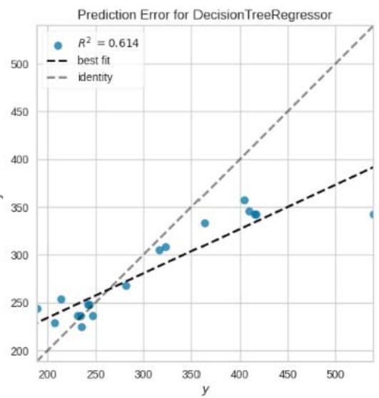Decision Trees Regressor Decision trees are a type of model used for both classification and regression. Trees respond to sequential questions which send us down a specific route of the tree. The model gets to produce decision for each feature, where each decision leads to a new question (decision) until a prediction is executed. {"algorithm_caption":[],"algorithm_content":[{"type":"text","content":"from sklearn.tree import DecisionTreeRegressor \n# Creating a Decision Tree Regressor model dt "},{"type":"equation_inline","content":"="},{"type":"text","content":" DecisionTreeRegressor(random_state "},{"type":"equation_inline","content":"\\coloneqq 42"},{"type":"text","content":" \n# Training the model dt.fit(x_train, y_train) \n# Making predictions on the test data y_pred_dt "},{"type":"equation_inline","content":"="},{"type":"text","content":" dt.predict(X_test) \n# Evaluating the model msec_dt "},{"type":"equation_inline","content":"="},{"type":"text","content":" mean_squared_error(y_test, y_pred_dt) r2_dt "},{"type":"equation_inline","content":"="},{"type":"text","content":" r2_score(y_test, y_pred_dt) msec_dt, r2_dt \n(5332.670754499999, 0.47899695889204263) "}]} Figure 7: Coding for Decision Tree Regression The Decision Tree Regressor model has a Mean Squared Error (MSE) of approximately 5332.67 and an R-squared $(R^2)$ score of 0.48 on the test data. This model's performance is significantly lower than the linear regression model. The $R^2$ score of 0.48 indicates that the model explains about $48\%$ of the variability in the target variable. ## iii. Random Forest Regressor Random Forest is a type of ensemble learning method, where a group of weak models cometogether to form a strong model. In Random Forest, we grow multiple trees as opposed to a single tree. To classify a new object based on attributes, each tree gives a classification. The forest chooses the classification having the most votes (over all the trees in the forest) and incase of regression, it takes the average of outputs by different trees. {"algorithm_caption":[],"algorithm_content":[{"type":"text","content":"from sklearnensemble import RandomForestRegressor \n# Creating a Random Forest Regressor model \nrf "},{"type":"equation_inline","content":"="},{"type":"text","content":" RandomForestRegressor(random_state "},{"type":"equation_inline","content":"\\coloneqq 42"},{"type":"text","content":" \n# Training the model \nrf.fit(X_train, y_train) \n# Making predictions on the test data \ny_pred_rf "},{"type":"equation_inline","content":"="},{"type":"text","content":" rf.predict(x_test) \n# Evaluating the model \nmse_rf "},{"type":"equation_inline","content":"="},{"type":"text","content":" mean_squared_error(y_test, y_pred_rf) \nr2_rf "},{"type":"equation_inline","content":"="},{"type":"text","content":" r2_score(y_test, y_pred_rf) \nmse_rf, r2_rf \n(3301.721138390172, 0.677421158517971) "}]} Figure 8: Coding for Random Forest Regression The Random Forest Regressor model has a Mean Squared Error (MSE) of approximately 3301.72 and an R-squared $(R^2)$ score of 0.68 on the test data. This model's performance is also lower than the linear regression model but greater than that of decision tree. The $R^2$ score of 0.68 indicates that the model explains about $68\%$ of the variability in the target variable. ### d) Combined Regressors by PyCaret PyCaret is a very robust Python library that will be used to compare different regression models and find the best one for our dataset. Firstly, regression module is set up in PyCaret with our dataset. Then, the compare Models function is used to compare different models. This function trains all models in the model library using cross-validation and evaluates performance metrics for regression, such as MAE, MSE, RMSE, R2, RMSLE, and MAPE. Another merit from this approach is that PyCaret library takes care of all the pre-processing steps such as missing value imputation, encoding categorical variables, feature scaling and normalization. This is shown as TRUE in figure 9 below. 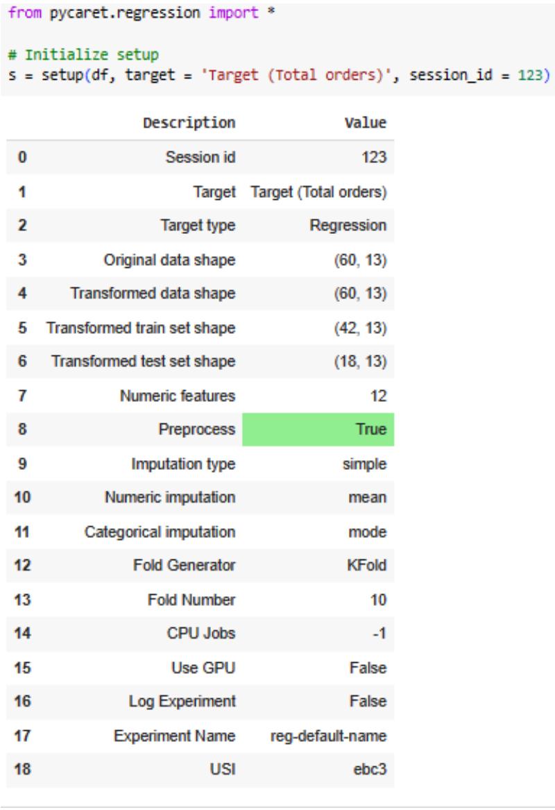 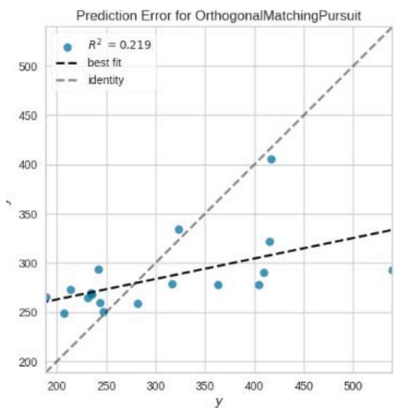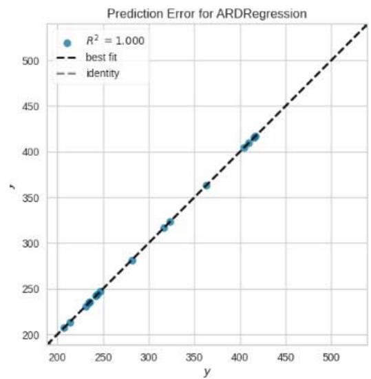Figure 9: Initializing PyCaret Regression Comparing all models best_model $=$ compare_models() <table><tr><td></td><td>Model</td><td>MAE</td><td>MSE</td><td>RMSE</td><td>R2</td><td>RMSLE</td><td>MAPE</td><td>TT (Sec)</td></tr><tr><td>lr</td><td>Linear Regression</td><td>0.0000</td><td>0.0000</td><td>0.0000</td><td>1.0000</td><td>0.0000</td><td>0.0000</td><td>0.2410</td></tr><tr><td>lasso</td><td>Lasso Regression</td><td>0.1612</td><td>0.0599</td><td>0.2003</td><td>1.0000</td><td>0.0006</td><td>0.0005</td><td>0.0320</td></tr><tr><td>ridge</td><td>Ridge Regression</td><td>0.0101</td><td>0.0005</td><td>0.0140</td><td>1.0000</td><td>0.0000</td><td>0.0000</td><td>0.0300</td></tr><tr><td>llar</td><td>Lasso Least Angle Regression</td><td>0.1613</td><td>0.0589</td><td>0.1998</td><td>1.0000</td><td>0.0006</td><td>0.0005</td><td>0.0310</td></tr><tr><td>br</td><td>Bayesian Ridge</td><td>0.0000</td><td>0.0000</td><td>0.0000</td><td>1.0000</td><td>0.0000</td><td>0.0000</td><td>0.0320</td></tr><tr><td>en</td><td>Elastic Net</td><td>0.2196</td><td>0.2108</td><td>0.3036</td><td>0.9998</td><td>0.0009</td><td>0.0007</td><td>0.0320</td></tr><tr><td>huber</td><td>Huber Regressor</td><td>13.1549</td><td>601.3146</td><td>18.2020</td><td>0.5207</td><td>0.0559</td><td>0.0409</td><td>0.0490</td></tr><tr><td>et</td><td>Extra Trees Regressor</td><td>18.9690</td><td>891.9745</td><td>24.7828</td><td>0.3170</td><td>0.0823</td><td>0.0657</td><td>0.1810</td></tr><tr><td>gbr</td><td>Gradient Boosting Regressor</td><td>19.8730</td><td>842.0865</td><td>25.1282</td><td>0.1901</td><td>0.0837</td><td>0.0684</td><td>0.0820</td></tr><tr><td>xgboost</td><td>Extreme Gradient Boosting</td><td>24.2394</td><td>1507.4219</td><td>32.4543</td><td>-0.0233</td><td>0.1033</td><td>0.0783</td><td>0.0520</td></tr><tr><td>rf</td><td>Random Forest Regressor</td><td>26.4847</td><td>1590.3080</td><td>34.5563</td><td>-0.3531</td><td>0.1075</td><td>0.0875</td><td>0.3490</td></tr><tr><td>ada</td><td>AdaBoost Regressor</td><td>27.1256</td><td>1507.4559</td><td>34.1499</td><td>-0.7393</td><td>0.1136</td><td>0.0940</td><td>0.0830</td></tr><tr><td>omp</td><td>Orthogonal Matching Pursuit</td><td>52.3762</td><td>4421.5898</td><td>59.9154</td><td>-1.5530</td><td>0.1948</td><td>0.1762</td><td>0.0300</td></tr><tr><td>dt</td><td>Decision Tree Regressor</td><td>36.5792</td><td>2991.5417</td><td>46.9773</td><td>-1.5823</td><td>0.1623</td><td>0.1238</td><td>0.0340</td></tr><tr><td>lar</td><td>Least Angle Regression</td><td>10.1883</td><td>472.8763</td><td>12.8457</td><td>-2.3624</td><td>0.0447</td><td>0.0380</td><td>0.0330</td></tr><tr><td>knn</td><td>K Neighbors Regressor</td><td>43.2565</td><td>4332.4947</td><td>58.0248</td><td>-2.4464</td><td>0.1783</td><td>0.1385</td><td>0.0310</td></tr><tr><td>lightgbm</td><td>Light Gradient Boosting Machine</td><td>61.1941</td><td>8041.0637</td><td>78.2081</td><td>-6.5747</td><td>0.2508</td><td>0.2113</td><td>0.0910</td></tr><tr><td>dummy</td><td>Dummy Regressor</td><td>61.1941</td><td>8041.0636</td><td>78.2081</td><td>-6.5747</td><td>0.2508</td><td>0.2113</td><td>0.0350</td></tr><tr><td>par</td><td>Passive Aggressive Regressor</td><td>125.4990</td><td>34680.1443</td><td>143.2859</td><td>-94.0216</td><td>0.3445</td><td>0.3983</td><td>0.0310</td></tr></table> The best model according to PyCaret comparison is the linear regression model. This is consistent with our earlier analysis where the linear regression model had an $R^2$ score of 1.0. However, as mentioned earlier, a perfect score is suspicious and could be a sign of overfitting, where the model has learned the training data too well and may not perform well on new, unseen data. It is important to note that PyCaret compare_models function uses cross-validation to evaluate the models, which provides a more robust assessment of the model's performance. Therefore, the linear regression model's perfect score in this case is less likely to be due to overfitting. The linear regression model seems to be the best model for predicting the weekly order volume based on the given features.  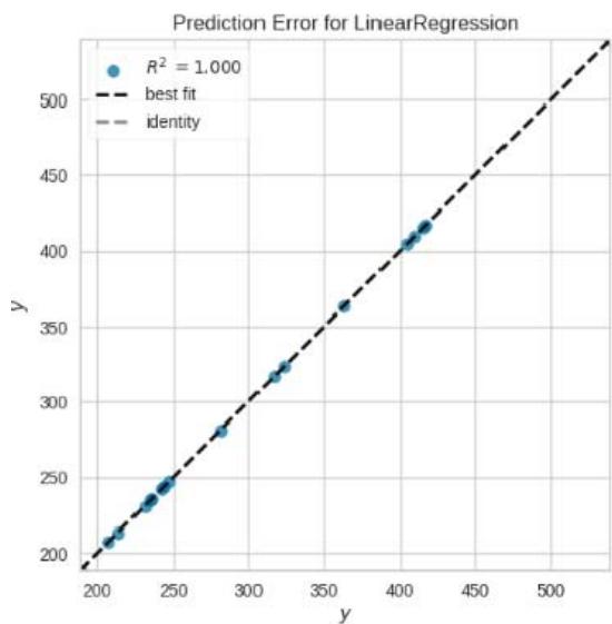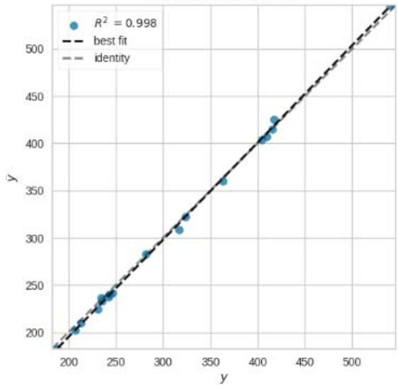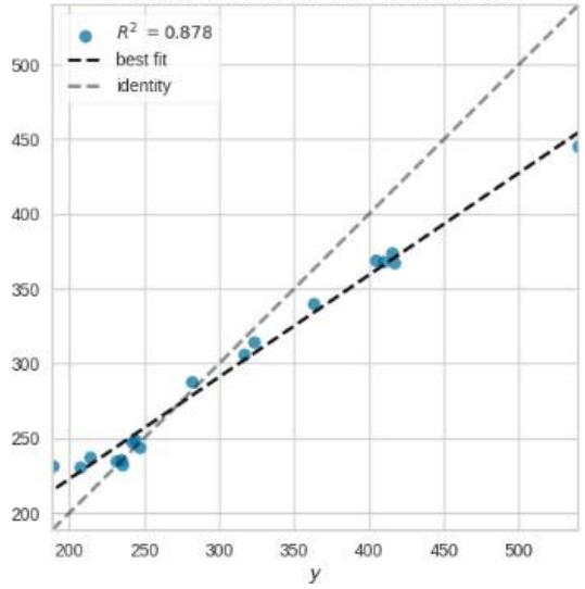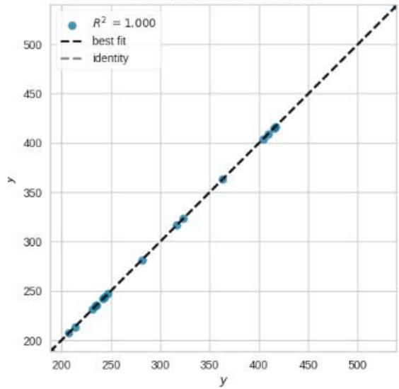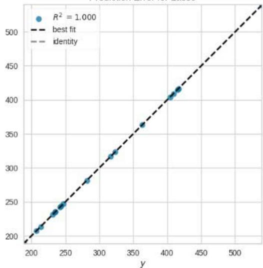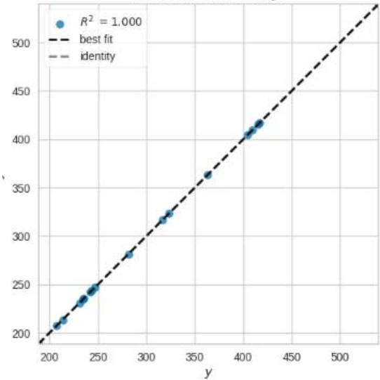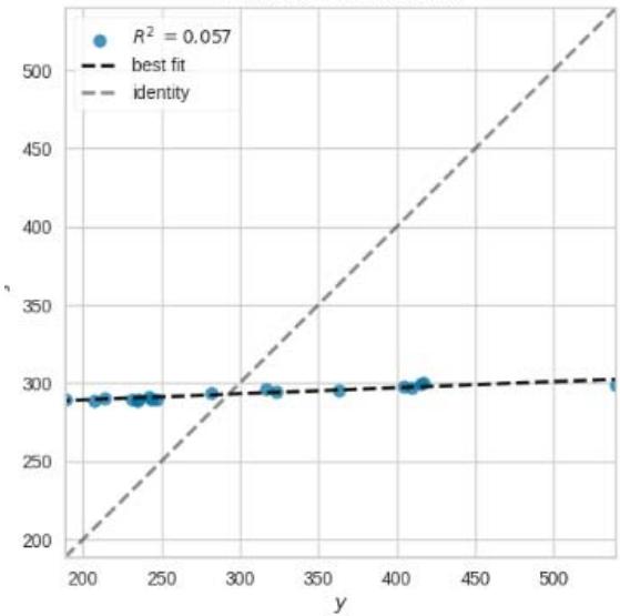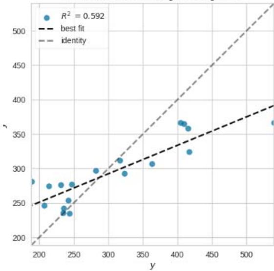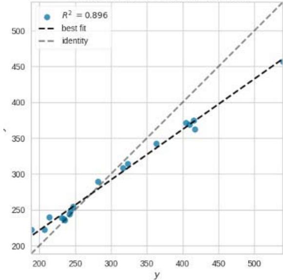Figure 10: Comparing Models from Eighteen Regressors   Prediction Error for RandomForestRegressor  Prediction Error for ElasticNet  Prediction Error for Lasso  Prediction Error for Ridge  Prediction Error for Lars  Prediction Error for LassoLars        Prediction Error for HuberRegressor  Prediction Error for KernelRidge  Prediction Error for SVR  Prediction Error for KNeighborsRegressor  Prediction Error for ExtraTreesRegressor  Prediction Error for AdaBoostRegressor     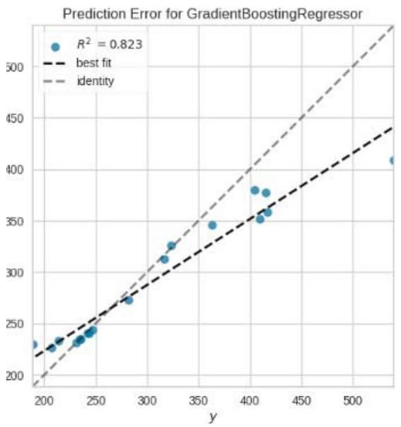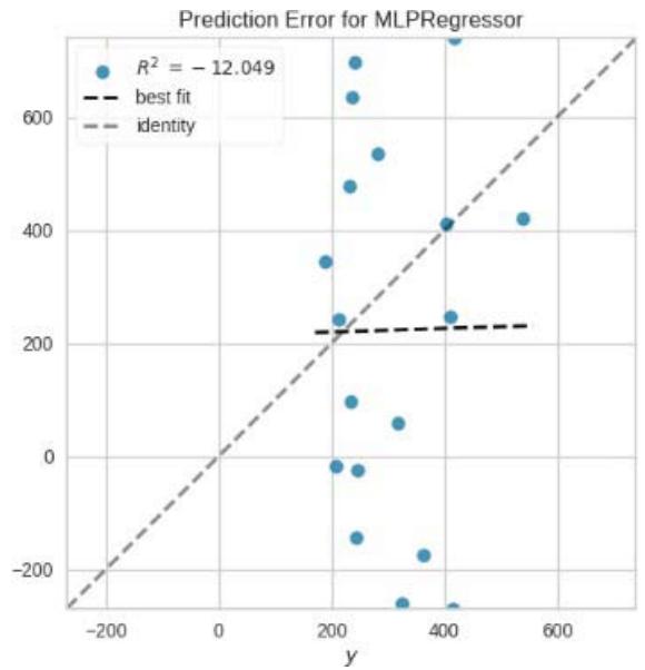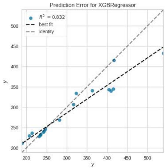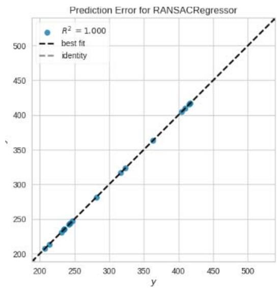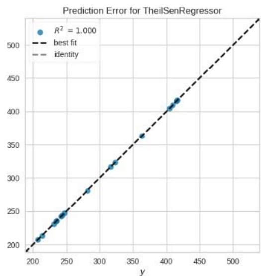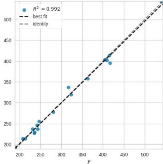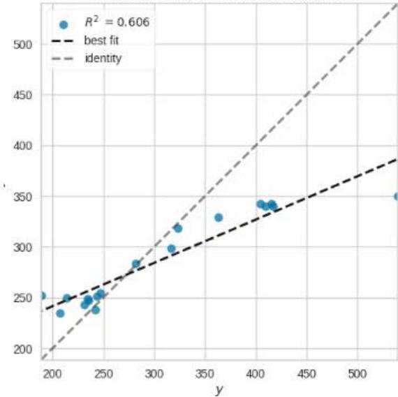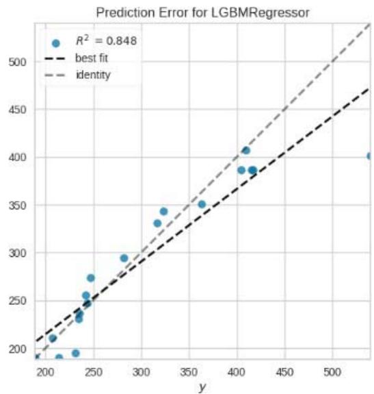Figure 11: Prediction Plots The feature importance plot shows the importance of each feature in predicting the target variable in the linear regression model. 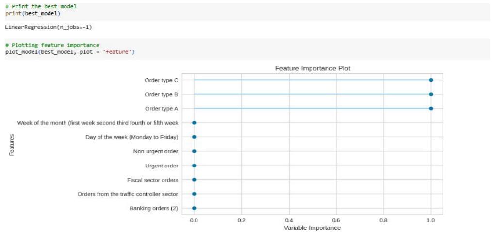 Figure 12: Feature Importance Plot From the plot, we can see that the most important features for predicting the total orders are: 1. Orders from the traffic controller sector (the most important feature, with the highest importance score). 2. Order Type C: This is the second most important feature. 3. Non-Urgent Order: This is the third most important feature. 4. Order Type B: This is the fourth most important feature. 5. Urgent Order: This is the fifth most important feature. a) Linear Regression (LR) The other features have relatively lower importance scores and they can be classified as less relevant in the study analysis. ## IV. RESULTS AND DISCUSSION From figure 10, we picked the first six models with smaller MAE and better predictions for discussion. The rest of the models from Huber Regressor to Passive Aggressive Regressor have high value of MAE and their predictions are less accurate. Table 1: Performance Parameters for Linear Regression Model <table><tr><td>Model Performance Parameters</td><td>Value</td></tr><tr><td>MAE</td><td>0.0000</td></tr><tr><td>MSE</td><td>0.0000</td></tr><tr><td>RMSE</td><td>0.0000</td></tr><tr><td>R2</td><td>1.0000</td></tr><tr><td>RMSLE</td><td>0.0000</td></tr><tr><td>MAPE</td><td>0.0000</td></tr><tr><td>TT (Training Time)</td><td>0.5810 seconds</td></tr></table> The linear regression model achieves perfect performance with MAE, MSE, RMSE, and RMSLE values of 0.0000, indicating that it perfectly predicts the target variable without any error. The $R^2$ value of 1.0000 suggests that the model explains all the variance in the data. ### b) Lasso Regression (LASSO) Additionally, the MAPE value of 0.0000 indicates that the average percentage error is zero. The training time (TT) is 0.5810 seconds, which is the time taken to train the model. Table 2: Performance Parameters for LASSO Model <table><tr><td>Model Performance Parameters</td><td>Value</td></tr><tr><td>MAE</td><td>0.1612</td></tr><tr><td>MSE</td><td>0.0599</td></tr><tr><td>RMSE</td><td>0.2003</td></tr><tr><td>R2</td><td>1.0000</td></tr><tr><td>RMSLE</td><td>0.0006</td></tr><tr><td>MAPE</td><td>0.0005</td></tr><tr><td>TT (Training Time)</td><td>0.0890 seconds</td></tr></table> The Lasso regression model achieves good performance with a relatively low MAE of 0.1612. The MSE and RMSE values indicate the average squared difference and square root of the average squared difference between predictions and actual values, respectively. The $R^2$ value of 1.0000 suggests that the model explains all the variance in the data. The RMSLE value of 0.0006 indicates a small average logarithmic error. The MAPE value of 0.0005 suggests a small average percentage error. The training time is 0.0890 seconds. ### c) Ridge Regression (Ridge) Table 3: Performance Parameters for Ridge Regression Model <table><tr><td>Model Performance Parameters</td><td>Value</td></tr><tr><td>MAE</td><td>0.0101</td></tr><tr><td>MSE</td><td>0.0005</td></tr><tr><td>RMSE</td><td>0.0140</td></tr><tr><td>R2</td><td>1.0000</td></tr><tr><td>RMSLE</td><td>0.0000</td></tr><tr><td>MAPE</td><td>0.0000</td></tr><tr><td>TT (Training Time)</td><td>0.0810 seconds</td></tr></table> The Ridge regression model performs very well with a low MAE of 0.0101, indicating a small average absolute difference between predictions and actual values. The MSE and RMSE values are also low, indicating a small average squared difference and square root of the average squared difference. The R2 value of 1.0000 suggests that the model explains all the variance in the data. The RMSLE and MAPE values are close to zero, indicating low logarithmic and percentage errors. The training time is 0.0810 seconds. ### d) Lasso Least Angle Regression (LLAR) Table 4: Performance Parameters for LASSO Least Angle Regression Model <table><tr><td>Model Performance Parameters</td><td>Value</td></tr><tr><td>MAE</td><td>0.1613</td></tr><tr><td>MSE</td><td>0.0589</td></tr><tr><td>RMSE</td><td>0.1998</td></tr><tr><td>R2</td><td>1.0000</td></tr><tr><td>RMSLE</td><td>0.0006</td></tr><tr><td>MAPE</td><td>0.0005</td></tr><tr><td>TT (Training Time)</td><td>0.0460 seconds</td></tr></table> The LLAR model performs similarly to the Lasso regression model, with a slightly higher MAE of 0.1613. The MSE, RMSE, $R^2$, RMSLE, and MAPE values are also comparable. The training time is 0.0460 seconds, which is relatively low. 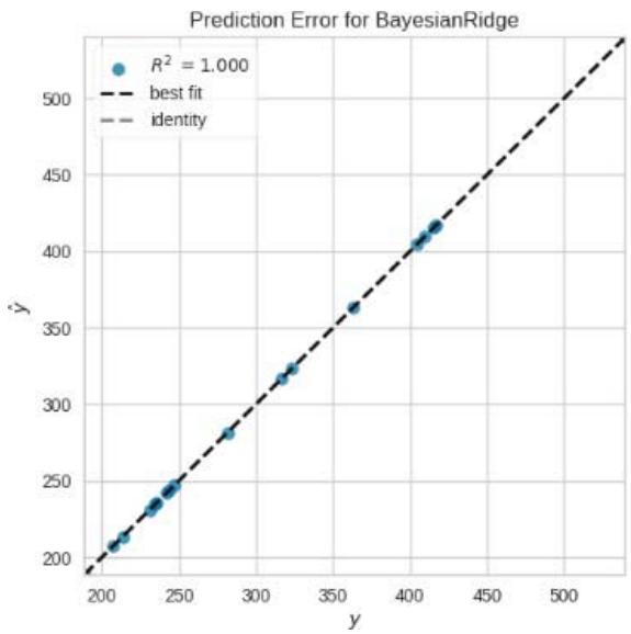### e) Bayesian Ridge (BR) Table 5: Performance Parameters for Bayesian Ridge Regression Model <table><tr><td>Model Performance Parameters</td><td>Value</td></tr><tr><td>MAE</td><td>0.0000</td></tr><tr><td>MSE</td><td>0.0000</td></tr><tr><td>RMSE</td><td>0.0000</td></tr><tr><td>R2</td><td>1.0000</td></tr><tr><td>RMSLE</td><td>0.0000</td></tr><tr><td>MAPE</td><td>0.0000</td></tr><tr><td>TT (Training Time)</td><td>0.0440 seconds</td></tr></table> The Bayesian Ridge model achieves perfect performance, similar to the Linear Regressionmodel. The MAE, MSE, RMSE, R2, RMSLE, and MAPE values are all zero, indicating perfect predictions. The training time is 0.0440 seconds. ### f) Elastic Net (EN) Table 6: Performance Parameters for Elastic Net Regression Model <table><tr><td>Model Performance Parameters</td><td>Value</td></tr><tr><td>MAE</td><td>0.2196</td></tr><tr><td>MSE</td><td>0.2108</td></tr><tr><td>RMSE</td><td>0.3036</td></tr><tr><td>R2</td><td>0.9998</td></tr><tr><td>RMSLE</td><td>0.0009</td></tr><tr><td>MAPE</td><td>0.0007</td></tr><tr><td>TT (Training Time)</td><td>0.0880 seconds</td></tr></table> The Elastic Net model performs relatively worse compared to the previous models, with a higher MAE of 0.2196. The MSE and RMSE values indicate larger squared differences and square roots of the squared differences, respectively. The $R^2$ value of 0.9998 suggests that the model explains most of the variance in the data. The RMSLE and MAPE values indicate small logarithmic and percentage errors. The training time is 0.0880 seconds. Overall, the Linear Regression, Bayesian Ridge, and Ridge Regression models achieve perfect performance with zero errors. The Lasso Regression and Lasso Least Angle Regression models perform well with low MAE values. The Elastic Net model performs relatively worse in terms of MAE but still achieves a high $R^2$ value. The training times vary among the models but are generally quite fast, with the longest being 0.5810 seconds for the Linear Regression model. ## V. CONCLUSION AND RECOMMENDATIONS This study illustrates a paradigm shift from traditional demand forecasting approaches to more sophisticated statistical methods and machine learning techniques. In line with these advancements, this study aims to improve existing knowledge on demand forecasting by utilizing an advanced Python library that simultaneously generates predictions using multiple regression algorithms. Additionally, the evaluation of the models' performance included various error analysis metrics such as MAE, MSE, RMSE, RMSLE, and MAPE. Among the models analysed, the first six models with smaller MAE and better predictions were selected for discussion. The remaining models, starting from Huber Regressor to Passive Aggressive Regressor, exhibited higher MAE values and less accurate predictions. The Linear Regression, Bayesian Ridge, and Ridge Regression models achieved perfect performance with zero errors across all performance metrics. The Lasso Regression and Lasso Least Angle Regression models demonstrated good performance with low MAE values. The Elastic Net model performed relatively worse in terms of MAE but still exhibited a high $R^2$ value, indicating a good level of explained variance. The training times varied among the models but were generally fast, with the longest training time observed for the Linear Regression model. This study builds upon previous research by employing advanced Python libraries and evaluating many regression algorithms simultaneously to improve demand forecasting. The selected models demonstrated varying levels of accuracy and computational efficiency. The findings highlight the effectiveness of non-linear techniques, such as Lasso Regression and Bayesian Ridge, in achieving accurate predictions with low errors. These results contribute to the growing body of knowledge on demand forecasting in supply chain planning and can aid decision-makers in improving their demand forecasting processes. It is very important to know the study dataset was small and there is propensity for few models to produce $R^2$ of 1.0000. The case will be different where we have voluminous dataset. Perhaps, based on the analysis and results obtained in this study, several recommendations can be made to further enhance the demand forecasting process in supply chain planning: 1. Explore ensemble methods: Ensemble methods, such as Adaboost and the ensemble of Random Forest, have shown promising results in previous studies. It would be beneficial to investigate the potential of combining multiple regression algorithms to create an ensemble model that leverages the strengths of different approaches and produces even more accurate predictions. 2. Other machine learning techniques: While this study focused on regression algorithms, there are other advanced machine learning techniques that can be explored for demand forecasting. For example, deep learning models like recurrent neural networks (RNN) and long short-term memory (LSTM) networkshave been successful in capturing complex patterns in time series data. Investigating the application of these techniques may lead to improved forecasting accuracy.

Generating HTML Viewer...

References

8 Cites in Article
Al-Jarrah Oy (2015). Efficient machine learning for big data: a review.
Real Carbonneau,Kevin Laframboise,Rustam Vahidov (2008). Application of machine learning techniques for supply chain demand forecasting.
M Casson (2013). Economic analysis of international supply chains: An internalization perspective.
Rohit Sanjay Pitale,Paras Arora,Charumani Singh,Darpan Malkan (2011). EVOLUTION OF UNITIZATION IN E-COMMERCE SUPPLY CHAIN.
David Ketchen,Larry Giunipero (2004). The intersection of strategic management and supply chain management.
J Hope,R Fraser (2003). Beyond budgeting: how managers can break free from the annual performance trap.
G Wang (2012). Unknown Title.
(null). Video for A Novel Dynamic Demand Forecasting Model for Resilient Supply Chains using Machine Learning.
No ethics committee approval was required for this article type.
Data Availability
Not applicable for this article.
How to Cite This Article
Tewogbade Shakir. 2026. \u201cEnhancing Demand Forecasting in Retail Supply Chains: A Machine Learning Regression Approach\u201d. Global Journal of Management and Business Research - A: Administration & Management GJMBR-A Volume 23 (GJMBR Volume 23 Issue A8).
Explore published articles in an immersive Augmented Reality environment. Our platform converts research papers into interactive 3D books, allowing readers to view and interact with content using AR and VR compatible devices.
Your published article is automatically converted into a realistic 3D book. Flip through pages and read research papers in a more engaging and interactive format.
Our website is actively being updated, and changes may occur frequently. Please clear your browser cache if needed. For feedback or error reporting, please email [email protected]
Thank you for connecting with us. We will respond to you shortly.