## I. INTRODUCTION In the B2B market we have seen for years an in equal relationships between customers and Suppliers. Suppliers deplore a behavior exclusively focused on costs, innovation capture, which in consequence generates an indifference to their recognizable values and push them to become a cohort of simple suppliers' commodities. Let's take the illustration of the European B2B automotive industrial environment which is a "hard industry and unrestrained when it comes to further increasing the pressure." (Roland Berger)[^1]. This industry is accustomed to exclusive pricing practice. The sector is now facing fierce Chinese competition, rising costs, end customer market hesitating adopt electric vehicles (EV). Facing these challenges, companies often take familiar patterns, favoring conservative approaches to cost management to the detriment of a value creation strategy. In this industry, generally speaking, finding solution, consist oneself to work on cost in order to manage change quickly in a controlled manner. Yet, let's take a more general perspective pointed out by Roger L. Martin2. In his famous HBR article in which he deplores the strategy of concentrating on costs, Martin talks generally about classical strategic planning failure concentrating on cost. We can ask, isn't it the same in most field business planning and where the same causes are responsible for the same effects? We are talking namely on tendency which has three major pitfalls: (1) expose an ambitious vision with a list of detailed and long initiatives that the firm must carry out to achieve the objectives and which are conditioned by the costs and the resulting financial performance. (2): concentrate on a cost way of thinking. (3) believe on a "self-referential strategic framework". This logic is particularly visible in B2B, where the fixation on the price-cost-volume triptych, inherited from Hirschmann's learning curve3 is no longer corresponds to current market dynamics according Montebello4. As Liozu[^5] and Montebello point out many manufacturing firms are still favorizing a revenue and volume approach instead capturing the value linked with an optimal price. In this way W. Chan Kim and Renee Mauborgne[^6] are highlighting that "Basic B2B industries..., taking it for granted that the product [...] is trivialized and that there is only one criterion on which to be beat, the price when in fact the factors of competition usually include evaluation and technical assistance services, delivery times, stock availability, etc.". However Hinterhuber and al., comment that B2B selling is undergoing a major shift, because it is not about communicating unique selling points (USPs) but more diagnose and propose solutions. Empirical studies (Ingenbleek and al)[^7]. $(2003)^{8}$ confirms that in the B2B, electronics and engineering sector, customer value-based pricing approaches are positively correlated with the success of new products, but nothing is said about recurring products. Monroe $(2002)^{9}$ observe that: "The profit potential of a value-based pricing strategy that works is far greater than any other pricing approach". Similarly, Hinterhuber which recalls Cannon and Morgan $(1990)^{10}$ recommend value-based pricing if the objective is profit maximization. Docters and al. $(2004, p. 16)^{11}$ consider value-based pricing to be "one of the best pricing methods". The Value-Based Pricing (VBP) approach is not simply an alternative, but a strategic approach to ensure sustainable competitiveness in a changing environment, VBP is based on a thorough understanding of the uncertainties and dependencies between the different variables influencing the perception of value. In this context, a Bayesian network approach is particularly relevant for modeling B2B pricing decision-making. In this article, we will explore how to combine the Bayesian approach with the uncertainties inherent in B2B markets. By setting out the factors of value perceived by the customer, the internal constraints of the company, the competitive dynamics, the evolution of demand, we want to put forward an approach that allows to provide solutions to values disclosure issues during B2B negotiation as per example Request For Quotation process. ## II. PRINCIPLES OF VBP Framing the principle of Value is still not an easy task. Just focusing on their temporalities is enough to understand that they are evolving and changing. This polysemy of values results in a difficulty of definition in management sciences. It is particularly true in context of pricing. Values must be placed around the frameworks which are specific to them. According to Forementini (2016), the B2B pricing process often offers vague description in literature. The literature review made by Formentini and All $(2016)^{12}$ allows to illuminate the Value-Based Pricing (VBP) concept, which is "the set of pricing methods used by the supplier to set the selling price around the value that a product or service can bring to its customers rather than as a margin added to costs" (Hinterhuber, $2004^{13}$; Hinterhuber, $2008^{14}$; Farres, $2012^{15}$ ). Nevertheless, there is not only the VBP in the pricing approach but also other methods like ABC, TC, KC, QBP and GBB which have been mentioned by Formentini and Mohamed $^{16}$ and which we summarize as follow: <table><tr><td>Activity-Based Costing (ABC) methods</td><td rowspan="3">What they have in common is that they concentrate the setting of the price in the hands of the customer and a market environment.</td></tr><tr><td>Methods for calculating target costing (TC)</td></tr><tr><td>Kaizen Cost Calculation Methods (KC)</td></tr><tr><td>Quality Based Pricing (QBP)</td><td>Based on the definition of quality criteria e.g. agricultural. Montobello17 combines value with perceived quality for the premium market.</td></tr><tr><td>Pricing for Good-Better-Best Pricing (GBB)</td><td>Based on an approach of increasing value through quality associated with price, but this is a consequence of a VBP.</td></tr></table> According Dutan (and All) $^{18}$, VBP is the most in-depth analytical approach to pricing but also and not a variable process that can be easily adjusted according to the customer, innovation or discounts. Due to all these reasons we will continue to focus on VBP in the full article. Indeed, the method it is recognized as profit margins driver because it aligns prices with perceived value of customer. However, the difficulty of implementing VBP persist as being sophisticated due to the customer specificities and complexity. Still organizations such as Sanofi-Aventis, SAP, BMW, among others, have adopted the advantages of VBP (Hinterhuber 2008) because VBP focus on customer's expectations and not just costs and competition. Based on our own research we can add the 3M company as well as Thales Group (military industry), Saint Gobain and Freudenberg (French and German Suppliers) in the list of VBP adopters. Nevertheless a 2008 survey (made by Hinterhuber) reveals that $44\%$ of pricing is based on competition linked to the inability of firms to quantify the value of the product and therefore stay simply hidden. In fact, not all VBP are applicable in all sectors neither. A 2021 study on the German sector recognizes that its implementation is facilitated in the technological sector but face resistance in the pharmaceutical industry (Steinbrenner-Turčínková[^19]). VBP poses also an organizational challenge and mainly in terms of remuneration of human resources. Hinterhuber argues salespeople, the first actors in pricing, should be remunerated in organization based on the level of profit generated and not just on volume which is usually the case. This puts VBP implementation in a disadvantage, which would require a governance decision to encourage profit in favor of an associated remuneration system. Understandably such a complex strategy need implementation toolkits. Thull[^20] and Liozu[^21], propose deploying VBP techniques based on step by step deployment like discover (in other words define references), diagnose (in other words list and select competitive advantages), design diagnose (in other words quantify and submit). It should be noted that the performance of VBPs is not widespread because only $5\%$ of firms are able to apply this philosophy (Art and Science). Liozias well as (Heiko Gebauer, Elgar Fleisch, Thomas Friedli) $^{22}$ assures the implementation is still difficult and often questioned because of asymmetrical captures of Values. In a commercial framework of supplier-customer values, values are based on a dialogue around shared elements. Not all values can be shared between seller and buyer because the objectives of the actors are opposed in a context of "exacerbated conflict". Indeed Pekka Töytäri, Risto Rajala, Thomas Brashear, Alejandro $^{23}$ explains, the more attractive is the VBP for customer, not necessarily more profitable it is for the seller. It goes without saying that like in the prisoner's dilemma, it has something to do with conflict illustrated by game theory in negotiation situations. This description of unbalanced deal translated into game theory language means a non-zero-sum game since a vcfair seller will want to sell a value to his customer at equal gains but the buyer. At the opposite the buyer want capture all value without consideration of it opponent. (Brennan et al., 2007)[24] speak of "zero-sum game" pricing. More rarely, the opposite phenomena of values captured by the seller come into play, but let us not exclude such cases. ### a) Non-Zero-Sum Games, Zero-Sum, Cooperation, Conflict-Negotiations In VNM's game theory logic, (VNM stands for Von Neuman-Morgenstern Oskar Morgenstern)[^25], nonzero-sum games are situations where the winnings and losses of the participants do not necessarily cancel each other out. Unlike zero-sum games, where the gain of one is exactly the loss of the other, non-zero-sum games allow outcomes where all participants can win or lose together. <table><tr><td>Zero-sum games</td><td>Non-zero-sum games</td></tr><tr><td>Losses and gains of the seller and customer cancel each other out. There is total conflict</td><td>Seller and customer gains and losses lose or win together</td></tr></table> ### b) Conflicts Related to VBP In a Customer-Supplier Gain-Loss relationship, in which an agonic context is inscribed, such a struggle corresponds to a zero-sum game. A conflict framework of agonic context corresponds to an asymmetrical situation and a competitive struggle where the seller wants to take advantage of the Client or the Client wants to take advantage of the Seller. In other words, the gain of one constitutes a loss of the other and can be include in pricing methods such as Activity-Based Costing (ABC), Target Costing (TC) and Kaizen Costs (KC). The interpretation of the conflict also reveals a cooperation where the value created by the seller satisfies the customer in a mutual gain and corresponds to a VBP Value Base Pricing. In itself, cooperation is everyone's benefit. <table><tr><td>Zero-sum game Asymmetric Agonic Conflict</td><td>Cooperation Symmetry</td></tr><tr><td>Non-Zero-sum game Dissymmetry Total Agonic Conflict</td><td>Zero-sum game Asymmetric Agonic Conflict</td></tr></table> The conflict table above is a synthesis of the negotiations conflict between an integration of profit solutions for the benefit (Distribution = Symmetry) of all and a distribution (Distribution = Asymmetry) for the benefit of some as defined by Dean Pruitt (1937-) Prius Mary parker Follet (1994) and Walton Mc Kersie (1965) $^{26}$ ### c) Negotiations In absolute terms the VBP found its efficiency in symmetrical negotiation. It is obvious that such a step is first and foremost an optimal result of a good negotiation but rarely the starting point. Before go further, we want to remind the theory of negotiations around the axes of chord symmetry, chord asymmetry, and chord asymmetry that are perfectly defined: 1. Symmetry: Corresponds to the Harvard-Model or Harvard concept which is the result of Harvard's University Law Scholl imagined in the 1970s in order to create a win-win situation. The American jurist Roger Fisher and the anthropologist William Ury conceptualized the goal of successful negotiation in the principles of the Harvard Concept contained in the book Getting to Yes in 1981. The BATNA Best Alternative to a Negotiate Agreement is the result, in other words, the question: "what is the best alternative if the negotiation fails?" BATNA also allows to sort out the best options and an alternative for each party. 2. Asymmetry: Corresponds to the theory of ripening in which different techniques, mediation, ripening, eagerness are engaged, when both parties realize that they are in a costly impasse motivated by a  catastrophe for which a possible just and satisfactory solution is needed. 3. Dissymmetry: Corresponds to an open conflict and corresponds to a point of no return. Druckman[^27] introduces the concept of the Turning Point to leave the conflict zone and represents a framework for interpreting the negotiation that allows us to analyze whether the discussion is moving towards a point of resolution or a standstill. In order to obtain a possible agreement, VBP is engaged in those different stages of negotiation which takes into account behaviors that change rapidly, allowing agents to reassess their positions and strategies based on new data that are essential to adapt the dynamic and strategic decision strategy in the various phases identified above. This makes it possible to update beliefs and strategies in real time and to model both symmetric and asymmetric relationships to correct a changing negotiation phase. For example, in a symmetrical negotiation, the parties may have equal mutual influences, while in an asymmetrical negotiation, one party may have greater influence over the other. This means that the agent can model the mutual influences between the different stakeholders and their respective positions. Adjusting conditional probabilities based on new information received allows beliefs and strategies to be updated in real time. Knowing these differences allows strategies to be adjusted accordingly so that negotiators can make more informed decisions by evaluating the assumptions of the different possible outcomes and get closer to an optimum. This makes it possible to better anticipate the reactions of other parties and to plan more effective strategies. ### d) Given Tools of Pricing Negotiations In negotiation, managers can rely on methods to target their prices and values (Hinterhuner & all.)[28] like the WTP (Winning Target Price), Price to Win (PTW) and RBV (Resource-Based View). In the area of price negotiation, there is a glimpse of an open scientific field. In the perceived reality, the framing of the price is done in coherence according to the experience of the firm agents which tracks price, costs, finance indicator history and possible customer feedback or don't disclose it: even luck. WTP, PTW and RBV have a very broad mathematical field that is essential in precise targeting of prices and values. We propose a synthesis of the mathematical tools implemented that unite and govern the models. <table><tr><td></td><td>Mathematical models implemented</td></tr><tr><td>WTP</td><td>1. Costing: Analysis of costs by evaluating direct and indirect costs associated with the production or provision of services.</td></tr><tr><td>PTW</td><td>2. Statistics: Mathematical regressions by comparison of available competitors&#x27; prices. Forecasting Models by using statistical techniques to forecast demand based on different price levels. 3. Logical: Mathematical optimization via programming maximization or minimization of objective functions under certain constraints via e.g. algorithms in order to find the optimal price that maximizes the chances of winning while respecting cost and margin constraints. For example, a Game Theory analysis via &quot;What-If&quot; Scenarios by evaluating the impact of different assumptions on the optimal price.</td></tr><tr><td>RBV</td><td>4. Qualitative: Valorization and temporal dynamics.</td></tr></table> We observe a deployment shift in the given tools and propose an additional perspective of ranking RBV, WTP and PTW in regards of temporality, which will show a split between tariffificationanteriority and active posteriority actions of negotiation. <table><tr><td>Temporality</td><td>Act</td><td>Type</td><td>Details</td></tr><tr><td>Ex-Ant</td><td>Tariffication/Preparation</td><td>RBV</td><td>An internally oriented preparatory process that helps assess internal resources prior to negotiations.</td></tr><tr><td rowspan="2">Ex-Post</td><td rowspan="2">Negotiation/Action</td><td>WTP</td><td>An externally oriented activity based on a target but not necessarily optimal price for the organization like in most Request For Quotation (RFQ)B2B Automotive</td></tr><tr><td>PTW</td><td>An externally oriented more geared towards finding the best optimal price based on values like in Request For Quotation (RFQ) B2G Military per example.</td></tr></table> If the applications of $\mathsf{RBV}^{29}$ are numerous applications in commercial, marketing, and entrepreneurship, however, the criticisms still remain against by questioning the capacity to differentiate in a competitive environment also due to its static and tautological aspect. Therefore, we suggest, among the three methods to keep PTW as the most actively incorporate in active negotiation to sale values. PTW combine efforts of collecting HUmanINTelligence (HUMINT) information _by sales managers_, analyze and work on the best price to win based on Open Source INTelligence (OSINT) on external and internal sources lead by PWT Managers. ### e) PWT Cross VBP As already said, the "Price Winning Target" (PWT) is a strategic approach that focuses on the optimal price to win. This method involves a thorough analysis of competitive prices, internal costs and the value perceived by the customer. In contrast, Value-Based Pricing (VBP) is a strategy that sets prices based on the perceived customer value of the product or service and less on production costs or competitor prices. This approach requires a thorough understanding of customers' preferences and the benefits of offered products or services. If the main difference between PWT and VBP is their focus: PWT centered on competitiveness while VBP is focused on maximizing profitability, in our opinion both approaches can converge on market and price: the PWT to set an optimal price according to costs and competition, the VBP to extract the most value from the price. This approach is not contradictory to the literature and shows the integrative capacity of VBP. We could interpret their convergences on the intersection: $\text{VBP} \cap \text{VBP} = (\text{Market}, \text{Price})$. Precisely the preferential choice methods included in PTW approaches, in a dynamic framework of pricing management in negotiation, which the B2B and B2G industry also use, can be those related to the Multiple-Choice Criteria Models (MCDM). MDCM extend the spectrum of criteria and variables and have a very high range of model (WSM, WPM, TOPSIS, etc.). We have studied them in detail and can therefore differentiate them between three types of approaches called MADM (A for Attribute), MODM (O for Object) and Uncertain. The main characteristic of MADM-MODM is around the forms of classification under distance and topology conditions; the main characteristic of the Uncertain is probabilistic and consists of fuzzy and Bayesian logics among others. (Figure 1).  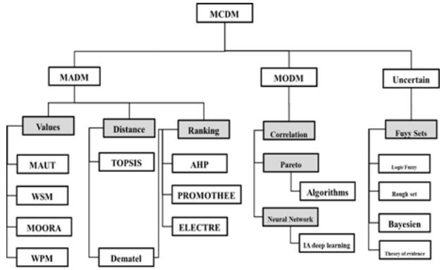Figure 1: MCDM Structure (by Author) ## III. MCDM APPLICATIONS IN NEGOTIATIONS In the field of strategic and complex negotiations, a particular form of method (MADM) called AHP (Analytic Hierarchy Process) is frequently used and recognized in the hierarchy of choices of complex decisions at several levels (Taherdoost) $^{30}$, (Stofkova and All) $^{31}$. AHP helps, for example, to select suppliers in a manufacturing company in India (Kamath & All.) $^{32}$ but also improve service quality in Healthcare $^{33}$. More specifically in the field of larger military, construction equipment Request for Quotation (RFQ) procurement use AHP which represents an effective strategic decision-making tool. Especially for the Business to Government (B2G) market and particularly for the Singapore Defense Industry of the Ministry of Defense (MINDEF) and the Armed Forces of Singapore (SAF) (Knowj Yoong Fui and Liam Hang Sheng) $^{34}$ AHP is an incomparable tool. The Analytical Hierarchy Process stems from the research of Thomas L Saaty $^{35}$ (1926 - 2017). The AHP allows a comparison using the same scale of ratios in intangible criteria in a hierarchy of choices to be evaluated by assigning them on cross-importance levels. The basis of a tool requires initial training but once acquired is simple to use. Thus, if we take the method in a negotiation framework, AHP helps to structure complex problems in a simple and clear way by taking into account the subjective preferences of decision-makers even during negotiation. Kiruthika and All $^{36}$ applied AHP to predict opponents' preferences in automated negotiations and were able to reduce the number of rounds of negotiation required to reach an agreement. In this way, the results of the AHP are transparent and easy to interpret, which can increase confidence in decisions. ### a) General Case Study We take the case of a competing firm on a B2B issued by an OEM (Buyer) for a Request for Quotation (RFQ) for a parts or system production and delivery (Seller). If the firm is in competition with other similar scaled competitors, we assume the customer's answers can be vague enough that perfect information cannot be transmitted to the salesperson. A PWT Team is in charge to evaluate the best VBP strategy in coordination with the Sales Team. Assumptions: we consider a supplier that produces semi-complex products. The firm is expected to produce A, B and C products with different levels of integration and profitability and that competitors do the same. Coalitions are not possible. The market is mature. The sector is not given specifically. The value of each firm is considered individually in the sense of a VBP. ### b) Deployment of the MADM AHP in PWT To conduct an AHP, a pairwise comparison matrix is constructed by following the following steps. The first action is to create a probability of dependence of the criterion ajon the criterion aji such that the subjective probability P (aij/aji) is determined on the basis of Saaty's table of subjective scores (Table 1). The pairwise comparison matrix makes it possible to evaluate the preferences of the criteria being compared on a scale ranging from 1 to 9 (H Taherdoost) $^{37}$. Table 1 Saaty Scoreboard 1. Equally important Preferred 2. Equal to moderate importance Preferred 3. Moderately important Preferred 4. Moderately to Strongly Important Preferred 5. Highly important Preferred 6. Strongly to Very Strongly Important Preferred 7. Very strongly important Preferred 8. Very strongly to Extremely important Preferred 9. 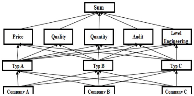Extremely important Preferred Let consider the simple case of a hierarchical negotiation on three levels opposite and adapted to the AHP approach of three firms in competitions (level 3) intra or extra-competitive, it does not matter, so that they can offer products (A, B, C) (level 2) on the values in typology of price, quantity, quality, response to audit and engineering note (level 1). The sum of the links represents the level 0. The First Step: On AHP consists by creating a probability of dependence of the ajj criteria on the aji criterion in the form of a matrix called the pairwise comparison matrix and which includes the subjective data collected between attributes. To fill the lower triangular matrix, the reciprocal values of the upper diagonal aji=1/ajare applied.  Prix\nAudit\nQuantity\nQualit\nLevel engineering <tr><td>Prix</td><td>Audit</td><td>Quantity</td><td>Quality</td><td>Level engineering</td></tr> Second Step: After normalization which consists dividing each element of the matrix by the sum of its column. A normalized relative weight is obtained. The sum of each column is 1. The resulting principal eigenvector of the matrix and noted by "w" is divided by the number n of criteria. In order to check the consistency of the response, the principal eigenvalue (also called maximal eigenvalue) is defined. The Principal Eigen Vector $\lambda$ max is obtained by summing the products of each element of the Eigen Vector and the sum of the columns of the reciprocal matrix. Saat a hghghdcproposes to use this index by comparing it to the appropriate coherence index which is called the random coherence index (RI). <table><tr><td>n</td><td>1</td><td>2</td><td>3</td><td>4</td><td>5</td><td>6</td><td>7</td><td>8</td><td>9</td><td>10</td></tr><tr><td>RI</td><td>0</td><td>0</td><td>0,52</td><td>0,89</td><td>1,11</td><td>1,25</td><td>1,35</td><td>1,4</td><td>1,45</td><td>1,49</td></tr></table> The consistency index (CI) allows to calculate the consistency of the structure on the basis of the number of criteria. $$ C I = \frac {\lambda_ {\operatorname* {m a x} - n}}{n - 1} $$ The ratio (CR) of the consistency index and the average consistency index should give a result of less than $10\%$, and in which case shows a coherence of the structure and the results of the comparison are acceptable. $$ C R = \frac {C I}{R I} $$ Final step: the goal is to hierarchy the importance of each variable so that the negotiator can handle in one direction or in another to structure the negotiation with consistence. The process is repeated as many possible interactions and for as many pairwise comparisons (1125=1*5*3*5*5*3_in case of the sample) as possible. Therefore, under the appearance of simplicity, the methodology is still heavy to exploit (Knowj Yoong Fui and Liam Hang Sheng)[^38] and is facilitate with help of specific software. AHP belong to rational decision models, which is an advantageous for explanation but has also flaws to exploit the full observable and hidden reality. Indeed as AHP belong to pure domain of MADM, it does not respond to the injunctions of uncertainty. The reality of the answers in a field negotiation suggests nevertheless uncertain events. In order to solve the problem of uncertainty, an improvement is often retained in the literature. Choices in uncertainty present propositions of AHP associated with fuzzy logic, that we are not going to study here, but which have the advantage of considering the uncertain, which AHP alone simply cannot regulate alone (Figure 2).  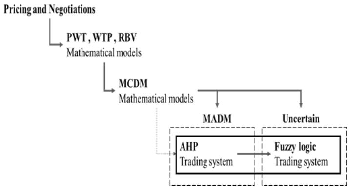Figure 2: Pricing and negotiations with MCDM Models (by Author) (Liu, Eckert, Earl) $^{39}$ (Ting-Ya Hsieh, Shih-Tong Lu, Gwo-Hshiung Tzeng) $^{40}$ (Jaskowski, Biruk, Bucon) $^{41}$ associate the AHP with fuzzy logic in the negotiation process. By using fuzzy numbers for linguistic terms or deflecting weights, we can see an aid in including value during negotiation. However, this approach is still anchored in a static nature, whereas negotiation evolves dynamically. While some examples prove the usage of MCDM-MADM_AHP tolls most currently negotiations under uncertain are frequently workout without any tool. We propose to change this approach with the support of MCDM-Uncertain. The Advantages and Disadvantages of AHP have been Demonstrated by Lui and Yang $^{42}$: On one hand, the method allows structured decision frameworkt which simplifies the understanding of complexity and improve clarify complex decisions. However, on the other hand, evaluation is limited and "leads decision-makers to make conflicting judgments. Finally, the results obtained by AHP are not fixed and, with the same hierarchical structure, decision-makers can create different evaluation matrices in different situations to obtain different evaluation results." (Lui and Yang). ### c) Improvement in Negotiations in the MCDM Field of Uncertain through Bayesian We have described fundamental characteristics in negotiations: (1) Modeling of Dependencies and Independence, (2) Management of Information Asymmetry, (3) Adaptation to Change, (4) Symmetry and Dissymmetry. These items can be handle by Bayesian Equilibrium and its capabilities extended of non-cooperative game theory $^{43}$. Bayesian is powerful tools in MCDM Uncertain for modeling and managing uncertainty in a variety of situations, including negotiations. In asymmetrical negotiation, the Luce-Raiffa matrix $^{44}$ (Figure 3) is a hypothesis according to which the opponents are able to correlate their strategies with communication, by transmit information to each other and agree on common point. This is a Bayesian game in which the information transmitted is understood by the opposing party which adapts its behavior a posteriori.  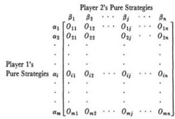Figure 3: Luce-Raiffa Matrix ### d) Bayesian Equality Before talking about Bayesian network, we must talk precisely about Bayesian equality, or Bayes' theorem, which is a fundamental formula in probability that allows to update the probabilities of previous events according to posterior information. It is expressed as follows: P (A|B) = [P(A). P (B|A)]/P(B) where: - (P(A|B)) is the probability of the event A knowing that B is true. - (P(B|A)) is the probability of event B knowing that A is true. - (P(A)) and (P(B)) are the probabilities of A and B independently. The search for a perfect equilibrium between A and B thanks to Bayesian equality makes it possible to correct the ex-Post actions to the ex_Ant actions of both. The Bayesian model of equality is based on principles of determinism and certain and uncertain stochastic graph theories, Markov theories. Discovered 261 years ago by the English Presbyterian pastor Thomas Bayes (1701-1761) and now extended in the broader form of modeling, commonly referred to as the Bayesian network, this tool represents an artificial intelligence whose goal is to offer a flexible and efficient tool for managing uncertainty. (CF. Figure 7) The Bayesian Network is a representation of graphs with nodes that are random variables and links that are influences from the basic mathematical model and as defined by Gonzales and Willein $^{45}$, whose "strength" lies in its influence to associate with probability distributions probabilistic expert system whose first advantage is to make prediction or diagnosis contrary to a classical determinism. - Prediction: The known causes what are the probable values of the consequences. - Diagnosis: Known consequences what causes are likely Classical determinism A B Bayesian determinism  B ### e) Bayesian Networks (BN) Classical analytical approaches tend to be based on a historical understanding of threat and risk datasets, and do not account for subjective assessments of how intelligent customers will change their strategies to be different from the historical model. Bayesian networks, also abbreviated by BN, overcome these limitations. The Bayesian networks are based on the seminal work of Pearl[^46] and Neapolitan[^47], including game theory and systemic applications of models and covers the entire field of linear and nonlinear systems. The theoretical basis of the BN and the Markov chain are conjoined through interference. A Markov chain is defined in a space $\mathbf{x}$ by the Transition Probability $P$ such that: $P(x\_n, x_{-}(n+1))$ once put end to end, this creates a sequence of random variables called Markov chain. The Markov chain has two behaviors of recurrence (state that once visited is visited an infinite number of times) and transient (state visited only a number of times). The basis of Bayesian Network Inference, as described in the literature by Neapolitan (2003), recalls that the sum of the actions of sets of events $X$ in time is equal to 1. The Bayesian structure satisfies the Markov condition if it has a single parent source. If such a structure has two parent s-sources, it is not Markov compatible. When a structure satisfies the Markov condition, then $P$ is equal to the product of its conditional distributions of all nodes given the values of their parents, whenever these conditional distributions exist. In such a way that when a structure is Markov compatible, we have to deal with a chain on which we can go up and down the frame of events and draw conclusions about inferences of ex-Post, ex-Ant events. Bayesian networks can be associated with different types of models depending on the amount of information available or not on the inner workings of the system. Bayesian networks can be affiliated with black-box, gray-box, or white-box models depending on the level of internal information available and used in the optimization process. 1. White Box Models: Are models with full transparency and where the inner workings of the system is fully known and can be used in the optimization process. 2. Grey Box Models: Are models which combines the black box approach with some internal knowledge of the system. For example, Bayesian gray-box optimization methods use partial information about internal calculations to improve performance. 3. Black Box Models: Are models which treat the system as completely opaque, meaning that you only the inputs and outputs without any knowledge of the internal processes are accessible. Classical Bayesian optimization often assumes a black-box approach. Unlike "black box" technologies such as neural networks, the variables and parameters of a Bayesian network are cognitively significant and directly interpretable. Bayesian networks use a logically consistent computation to manage uncertainty and update conclusions to reflect new evidence. There are processable algorithms to calculate and update the evidentiary support for the hypotheses of interest. Bayesian networks can combine data from a variety of sources, including expert knowledge, historical data, new observations, and results from models and simulations. These information's are coming from experts to build the structure while being very flexible. The structure is the first step in building a Bayesian network. We repeat it needs a small group of experts capable of identifying the different processes of complex risk selling in order to truly build the structure capable of predictions. Bayesian networks offer a structured and flexible approach to managing negotiations, taking into account information asymmetries, dynamic changes, and complex dependencies and dependencies by disclose Visible and Hidden events. Oliehoeket (2012) $^{48}$, links Bayesian networks, non-zero-sum games and cooperative games, showing methodologically how probabilistic structures and coordination graphs can be used to model and solve multi-agent decision-making problems in uncertain environments corresponding to business negotiations. ### f) Connecting the Dots of Values According Brechet[^49], values are data such as those of the market, such as price, quantity, physical data... but values are also ambiguous because they are given and first constructed specifies. We would like to add that they are also subjective. This is why we can share (Liozu)'s[^50] vision around the principle of VBP is a combination of art and science. Valuesare also built around the principle of mimicry of a conventional agreement (Gomez 1994, 1996)[51] which is based on a form of learning (René Girard) and motivation (Albert Bandura) of the agents of the internal and external organization. Therefore, values are a combination of data constructed in science and in subjectivity and recalls Liozu and other expression about a conjunction of Scien and Art. In an evaluation of values, the Bayesian approach has the advantage of taking into account both the constructed and subjective data that represent the values. Bayesian equality can be used to evaluate optimal strategies based on the information available in a complex B2B sales negotiation framework. For example, in a game where players must decide whether to cooperate or betray, they can use Bayes' theorem to estimate the probability that the other player will cooperate, based on previous information and observed behaviors. The representation in the form of Bayesian has a frequency aspect. A repetition of observations can be a set of at different times. The network "constitutes a representation of the model during a certain number of periods", as shown in the figure (Figure 4), which is similar to a series of known or anticipated events.  Figure 4: Simple Bayesian Model Illustration (By Author) When several events follow one another, a Bayesian network allows events to be linked together, the Markovian character of Bayesian networks makes it possible to take into account the temporal link between events that can be linked. To be more precise, it is a contortion of possibilities over time in search of spectrum of solutions in a space of interconnected values in the form of superimposition of logical "layers" integrating levels to be reached and not exceeded. In this we will have an overall ex-Post logic but with an additional variability of the complete ex-Ant network without having to go through a financial body but perfectly integrated into the topology of negotiations over time. Concretely, create a temporal hierarchy related to the occurrence of values and create nodes (Figure 5). Potential impacts of each value node are scaled around their impacts. If the impacts are not known, elicit them. The network will be oriented according to the temporal hierarchy (from top to bottom) and will take into account the potential impact (from left to right).  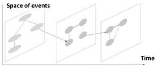Figure 5: Negotiation (Time Axis) in Bayesian form (Space Axis) (By Author) This represents a paradigm shift because the model does not sacrifice the interactivity of events with each other at the cost of an intrinsic simplification that is very often observed, but preserves them by comparing them. ### g) Bayesian Network and Human Logic Pearl and Kim are both pioneers of Bayesian Network and Artificial Intelligences $^{52}$. Back in 1983 both had point out the closeness of prospect theory (Kahneman and Tversky $^{53}$ ) with Bayesian logic. BN provides the theoretical foundations that show how humans decide behavior find it natural way to think in terms of Manifestation $\equiv$ Cause rather than in terms of Cause $\equiv$ Manifestation. To be more specific, let's assume an example of B2B negotiation, between a seller and a buyer based on a quantity (Q) of parts [p] at prices (P). If the selling agent offers the buying agent the price (P) of a [p] composed of different materials and offers him a final price but calibrated to the variability of the material indices (I) of [p]. According to the terms of the prospect theory (Kahneman-Tversky), the majority of buyers would prefer to play the confidence game with a predictable and therefore fixed price rather than an adjusted pricing that is considered risky according to the agents since they lack confidence in the predictions of the variability of the index. In prospective terms, this corresponds to the natural tendency to overestimate potential losses against potential gains. This leads to a preference for safer and more predictable options. Indeed, taking into account the lessons of prospect theory, we know that agents evaluate economic decisions according to their own reference and in the framework of uncertainty in which they make their decisions. Let's playnow the event A which precede event B. In the human understanding of priors, the relationship Manifestation $\coloneqq >$ Cause (acc.Kim-Pearl) corresponds to an intuitive logic $B = >A$, i.e. it is a logic of plausibility facilitated with similar examples and experiences that come to mind and correspond to heuristics (Kahneman & Tversky). The relationship Cause $\coloneqq >$ Manifestation corresponds to an $A = >B$ logic, i.e. it is a so-called a posteriori logic and rather counterintuitive. Thus, by respecting the conditions of Bayesian logic, the logic of intuitive plausibility naturally interpreted P (B/A, C) by humans can be revised to the level of the a priori laws observed on unknowns, and following updates when the system will provide more information, will give the law a posteriori which is counterintuitive and corresponds to a relationship Cause $\coloneqq >$ Manifestation as follow: $$ \text{LawaPosterior} \propto \text{LawaPriori *} \quad \text{Probability} $$ $$ P(A / B,C) \propto P(A / C) \star P(B / A,C) $$ Consequently, back to example, all the ambiguity of the buyer about price value is due to the index which corresponds to a plausibility that does not make evident sense to him. However, he should rather calibrate his interpretation to the law a priori by taking in account the occurrence the material index in such a way that it never loses. In the complex case of the interaction between several causes, Kim and Pearl propose Bayesian model as a formalization to reflect humans' causal perceptive relationships, while maintaining computational efficiency and remaining consistent with the principles of probability theory. The model captures interactions between multiple causes using conditional probabilities and local belief updates like downstream observed data and influences the probability of a cause and reinforces the evidence of the diagnosis. The model described by Judea Pearl and Jin H. Kim has directly influenced the development of Bayesian networks, such as Directed Acyclic Graphs (DAG), Conditional Probability Tables (CPTs), Belief Propagation, Messages used to propagate information through the network, conditional independence (Bayesian networks exploit the properties of conditional independence to simplify calculations) and finally Inference and Learning. That is to say, to calculate the probability of a given variable according to certain observations. This last point is crucial because through learning, Bayesian networks can fit the model parameters (conditional probabilities) based on the observed data. Consequently, Bayesian logic takes into account human logic but readjusts it by the rational logic of observation, to correct a logic that would be eventually counterintuitive and biased. After adjustment on a large number of variables that traditional decision models are not able to handle BN help readjust the truth. Bayesian networks represent a step forward in complex thinking because of their counter-intuitive characteristics. 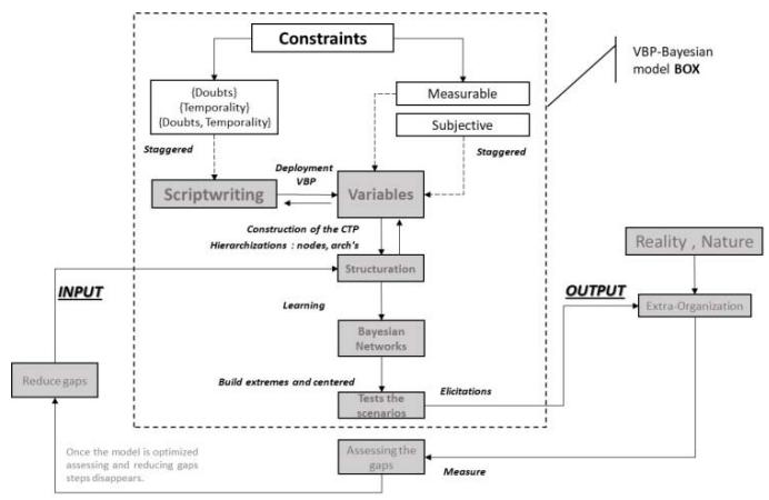### h) Deployment of Bayesian Network in PWT The most important understanding of Bayesian network is that it can help reinforce the possibilities of obtaining best possible VBP during a complex negotiation which extend over a topology of different events like eBay (electronic auction), CBD (Cost Break Down), face-to-face negotiation, which are all different in term of temporality, product, program and customers. In order to not exclude or include core input elements allowing to influence nodes decisions, it is equally important to understand that the dynamic over time improve the network (System) though its own learning processes. That haven been written, the deployment of a Bayesian Network will have to follow a certain number of rules. We will bring up some according recognized by Highest Bank authority (Federal Reserve Bank of Richmond) and exposed in literature of Bank Risk Finance Model (Naim, Condamin $^{54}$ ). The first and foremost priority is to establish a core team of Experts (Figure 6) equivalent to a Delphi group. We consider a Core team to be made up of members of the VBP and PWT members of Sales team and "flying agents" for particular purpose of collecting and distribution hidden information's. The total number of agents should according us not exceed 10 or 15 according (Hackman) $^{55}$ agents for reasons of uncontrolled noise and mimicry within this small structure.  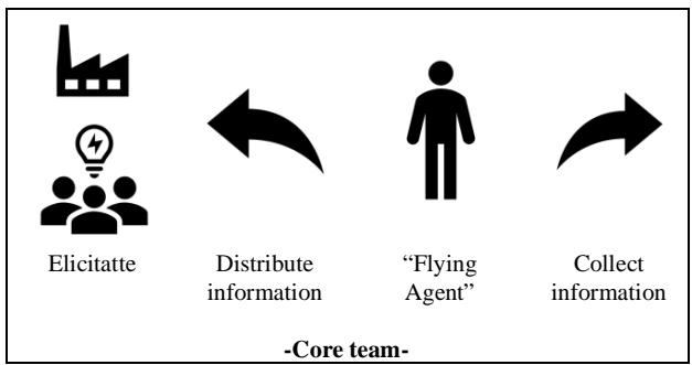Once the expert team has been implemented within the organization or a laboratory, the objective will be simulating the scenarios most likely to succeed. As well it is crucial to include a mediator (Raiffa $^{56}$ ) which rule is an arbitrator and facilitator of the full methodology. Pricing managers as well as sales executives will have then to follow the algorithm of Bayesian Network deployment (Figure 7) which represent the architecture of multiple specific steps we will detail through an example.  Figure 7: Algorithm deployment of a Bayesian Network in VBP (By Author) ### i) Construction of the Bayesian Network in PWT In a VBP pricing framework a Bayesian network can effectively handle both known and unknown variables and is able to improve precision thanks to the incorporation of prior knowledge and updating of new data. The major problem arising will result in the relationship between variables that influence values and price. Therefore, the level of precision will be adapted to the subsequent experiment decision. To be more specific: once the variables of the Bayesian network are defined, by the experts, a CPT (Conditional Probability Table or also described as Conditional Possibilities Distribution in literature) can be define. The CPT could include for example in a complex B2B negotiation, the ability to produce types of parts, the quality of suppliers, the distance to the customer (physical values), the subjective internal and external culture distance. The variables corresponds to the edges and nodes of the structure which, once interconnected according to their occurrence rates, will be linked in a Bayesian structure in the form of a DAG (Directed Acyclic Graph). CPT and DAG are the backbone of every Bayesian Network <p>CPT and DAG are the backbone of every Bayesian Network</p> While building the network the expert group will have to carefully take care not overload the size of attributes and set manageable scenarios so as not to overcomplicate and no longer measure results avoiding ambiguity. The consistency ratio reaches limits when the number of parameters exceeds 10 and the subjective nature of dependencies therefore it is advised to keep them between 5 and 10. It is recommended to optimize the model where impacts and occurrence are better defined with less parents. Reducing the number of parents per variable and connections (the arcs) is a primary objective in order to avoid overtraining (Vapnik) $^{57}$ but must also correspond to enough observations to validate the variables (James) $^{58}$ (Hastie) $^{59}$ (Burnham) $^{60}$ to justify a deterministic and stochastic prove of correlations. Once the references have been established, it is question of taking up the principles of VBP deployment according to Hinterhuber $^{61}$ and Thull $^{62}$ which cross the statistical deployment (Schmueli $^{63}$ ) by following process: defining the goals $\succ$ studying and collecting the data $\succ$ preparing the data $\succ$ exploratory of data analysis $\succ$ choose variables and built the model according to the Trinity of boxes of a Bayesian Modeling process in order to test the adaptation of a Bayesian model to VBP pricing in B2B request for quotation. ### j) Application of Uncertain Bayesian Network in PWT We use the same example also used on the AHP method to illustrate how does work a BN. To simplify, we only take the case of one firm (company A) among the three presented and for one type of product (Type A) among the three, to quantify all the dependencies with respect to the Level Engineering criterion by adding, for more precision on the level of vertical integration (product/process) of this product (see image on the left). The model we get is a naive Bayesian model. A Naive Bayesien model applies the Bayes Theorem, when, letAi be the possible arguments and Ci the corresponding criteria, the ranking of the arguments A and criteria will follow a logic such as: $$ P(Ci/Ai) = P(Ci).P(Ai/Ci) / P(Ai) $$ ### k) Metavariables in Relation with PWT Bernard Roy (1934 - 2017) $^{64}$, French pioneer in "decision making" and inventor of the ELECTRE method, emphasizes that approximation of criteria has to be considered as a reality. In such way even imprecise information is not necessarily rejectable. Therefore, notions of discrimination thresholds and pseudo criteria as parameters are to be considered. In the context of BN it suggests there are no fixed meta-variables as BN represent model and a probability distribution. According Roy "A model is a schema which, for a field of questions, is taken as a representation of a class of phenomena, more or less skillfully removed from their context by an observer to serve as a support for investigation and/or communication." The BN logic is based on observed dependency relationships between variables which create metavariables. Constraints fixed Meta-variables in advance would contract the Bayesian logic flexibility. However, sampling technics highlight the way to disclose metavariables. #### Sampling Meta-Variables There is a number of relevant intangibles to update beliefs about variables. We highlight some of them that could be collected and we propose to classify according their level of deduction, induction, subjectivity: #### Definitions: - Deduction: Which can be directly measured and verified by objective data. - Induction: Based on repeated observations and experiments and less accurate than deductible values but can be estimated from historical data - Subjectivity: Depend on individual perceptions and can vary from person to person. They are more difficult to quantify and standardize. <table><tr><td>Direct Observations</td><td>Latent Variables</td><td>Market Indicators</td><td>Behaviors and Reactions</td></tr><tr><td>Deductive [De]</td><td>Inductive [In]</td><td>Inductive [In]</td><td>Subjective [SU]</td></tr><tr><td>- Prices offered and accepted. - Quantities of goods or services traded. - Specific conditions of the negotiation (dead-lines, payment terms, etc.).</td><td>- Estimates of marginal costs or profit margins. - Agents&#x27; preferences (buyer and seller) regarding the terms of the negotiation.</td><td>- Commodity price indices - Relevant economic or sectoral trends.</td><td>- Agents&#x27; reactions to proposals and counter - proposals. - History of past negotiations - Patterns of behavior.</td></tr><tr><td>Hard Dependence</td><td>Strong Dependence</td><td>Strong Dependence</td><td>Fuzzy Dependence</td></tr></table> The following case study will help to better understand the deployment of meta-variables sampling. 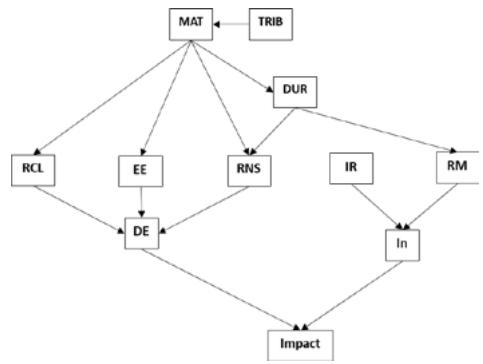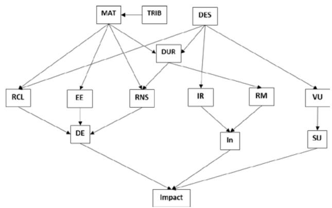#### 1) SKF Case Study We propose to take up of SKF(a Swedish ball bearing company) documented case in literature by Hinterhuber and All in "Value First, The price, Building base Valued-Baes princing strategies". In this illustration, Hinterhuber and All present the values that have been determinate according "a value calculator to document to customers the customer's next best alternative" to demonstrate how SKF has managed to convince their customers of the higher value of their products despite a higher price. By doing the work backwards based of resulting SKF values, we can show how to build a Bayesian network. Indeed, in normal case, Bayesian Network construction framework leads to obtain values. Of course, this represent an ex-Ant approach which could be criticized by being a typical case of intuitive logic $(\mathsf{B} = >\mathsf{A})$ of plausibility. We do not make this mistake because we are only re-establishing a structure on the basis of real answers by reducing all other speculations. The work of counter factuality (against time) that we carry out is based consequently on the search for possible dependencies, i.e. the a priori laws that are the opposite of biases. We give abbreviations to 6 values highlighted in the SKF case study: <table><tr><td>Valeur 1</td><td>Valeur 2</td><td>Valeur 3</td><td>Valeur 4</td><td>Valeur 5</td><td>Valeur 6</td></tr><tr><td>Reduced Lubrication</td><td>Energy Savings</td><td>Inventory Reduction</td><td>Faster installation</td><td>Increased Reliability and Durability</td><td>Process Optimization</td></tr><tr><td>(RCL)</td><td>(EE)</td><td>(RNS)</td><td>(IR)</td><td>(RM)</td><td>(UL)</td></tr><tr><td>SKF has shown that its bearings reduce lubrication costs, which translates into cost savings for the customer.</td><td>SKF bearings are more energy-efficient, saving customers money on their energy bills.</td><td>By using SKF products, customers can reduce their inventory levels, which lowers inventory management costs.</td><td>SKF bearings are designed for faster installation, which reduces downtime and improves operational efficiency.</td><td>SKF products offer superior reliability and durability, which trans-lates into lower maintenance costs and less frequent replacements.</td><td>SKF helps customers optimize their production processes with tailor-made solutions, which improves overall efficiency</td></tr></table> The majority of the values described in the SKF case study correspond to use and management cases that we group in Use value = {Reduction in lubrication operational costs; Energy saving; Quick installation; Maintenance; Versatility of use} and Management value = {Inventory level reduction}. From this on we can classify values into categories according to their level of deductibility (logos), inductility (experience), subjectivity (feeling): <table><tr><td>Deductive [De]</td><td>Inductive [In]</td><td>Subjective [SU]</td></tr><tr><td>(RCL)</td><td rowspan="2">(IR)</td><td rowspan="3">(VU)</td></tr><tr><td>(EE)</td></tr><tr><td>(RNS)</td><td>(RM)</td></tr></table> By adding causality parent elements, we extend the structure of the Bayesian network to a higher level to hypothetically create the conditions that act on Bayesian networks. Since we cannot speculate, we look in the document to see if it provides us with causalities related to the identified values (RCL, EE, RNS, IR, RM, VU). <table><tr><td></td><td>(RCL)</td><td>(EE)</td><td>(RNS)</td><td>(IR)</td><td>(RM)</td><td>(VU)</td></tr><tr><td>Parent Causality</td><td>SKF bearing design</td><td>Energy efficiency of SKF products, which consume less energy during operation</td><td>Reliability and durability of SKF products</td><td>Design of SKF products, which are optimized for fast and efficient installation</td><td>Resulting from the high quality and durability of SKF products</td><td>Flexible design of SKF products</td></tr><tr><td>Child Consequence</td><td>Reduced Lubrication</td><td>Energy Savings</td><td>Inventory Reduction</td><td>Faster installation</td><td>Increased Reliability and Durability</td><td>Process Optimization</td></tr></table> However, the case study only mentions the values of SKF products without specifying reference quantities. We can therefore propose a possible dependence by formulating the hypotheses on the basis of a logical syntax by grouping them into three groups: Materials (MAT), Design (DES), Durability (DUR). Indeed, the materials (MAT) chosen allow for greater energy efficiency (EE) since from the optimization but also the limits of the tribological nature (TRIB) which also has an influence on the durability of the products and therefore the stock (RNS). The design (DES) alone allows for faster installation (IR) as well as process optimization (VU) and combined with materials ensures a reduction in the lubrication level (RCL). Finally, durability depends on materials (MAT) and design (DES) and influence reliability (RM) and level (RNS). From the statistical collection, customer satisfaction, the organization will be able to build the conditions for value creation as follow: 1. The dependencies from which the parent (MAT) derives are of the order of engineering science. 2. The dependencies from which the parent (DES) derives are of the order of customer use and therefore oriented towards Sales, Service, Marketing, Quality For example, dependency (DES/IR), which is an induction, can be obtained by precise questioning of the customer cohort on the basis of targeted questions such as customer complaint feedback on various technical points. At this points we can create two types of DAG: a DAG which include Engineering Sciences and a DAG which include (Sales, Service, Marketing, Quality). Such a DAG makes it possible to obtain the results of a system but it must be built on the synergy of deductions number of sub-assemblies of the organization: and inductions, which implies the work of a large engineering, sales, service, marketing, quality.  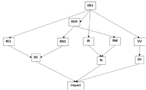DAG Engineering Sciences  DAG Sales, Service, Marketing, Quality By grouping these elements together, the complete DAG is obtained.  Panel label: Full DAG. We can continue to construct a Conditional Probability Table (CPT) by considering the scales and build up the BN. Variables - Values STATES Description Materials (MAT) Conditions: Wear-resistant, Lightweight, Standard Description: Materials can be wear-resistant, lightweight, or standard. Design (DES) Statuses: Optimized for Efficiency, Standard Description: The design can be optimized for efficiency or standard. Durability (DUR) Status: High, Medium, Low Description: Durability can be high, medium, or low. Réduction des Coûts de Lubrification (RCL) States: Yes, No Description: Indicates whether or not lubrication costs are reduced. Energy Saving (EE) States: Yes, No Description: Indicates whether or not energy savings are being achieved. Quick Installation (IR) States: Yes, No Description: Indicates whether or not the installation is quick or not Reduced Maintenance (RM) States: Yes, No Description: Indicates whether or not maintenance is reduced. Versatility of use (VU) States: Yes, No Description: Indicates whether the product is versatile or not. Reduction of Stock Level (RNS) States: Yes, No Description: Indicates whether or not inventory levels are reduced. <table><tr><td>Variables - Values</td><td>STATES</td><td>Description</td></tr><tr><td>Materials (MAT)</td><td>Conditions: Wear-resistant, Lightweight, Standard</td><td>Description: Materials can be wear-resistant, lightweight, or standard.</td></tr><tr><td>Design (DES)</td><td>Statuses: Optimized for Efficiency, Standard</td><td>Description: The design can be optimized for efficiency or standard.</td></tr><tr><td>Durability (DUR)</td><td>Status: High, Medium, Low</td><td>Description: Durability can be high, medium, or low.</td></tr><tr><td>Réduction des Coûts de Lubrification (RCL)</td><td>States: Yes, No</td><td>Description: Indicates whether or not lubrication costs are reduced.</td></tr><tr><td>Energy Saving (EE)</td><td>States: Yes, No</td><td>Description: Indicates whether or not energy savings are being achieved.</td></tr><tr><td>Quick Installation (IR)</td><td>States: Yes, No</td><td>Description: Indicates whether or not the installation is quick or not</td></tr><tr><td>Reduced Maintenance (RM)</td><td>States: Yes, No</td><td>Description: Indicates whether or not maintenance is reduced.</td></tr><tr><td>Versatility of use (VU)</td><td>States: Yes, No</td><td>Description: Indicates whether the product is versatile or not.</td></tr><tr><td>Reduction of Stock Level (RNS)</td><td>States: Yes, No</td><td>Description: Indicates whether or not inventory levels are reduced.</td></tr></table> ### m) Practical Structuration to Generate Values Once meta-variable logic have been set up we propose create a CPT based on the AHP example. It should be noted that the way of building a Bayesian network is dependent on the links of distributive estimates, regression logic, and Boolean law. Then we estimate and specify the conditional probability distribution of the various sources of information. In Bayesian networks, variables can be discrete has a finite number of values or a continuous which has an infinite number of values between two limits. Let's consider the Basic structure (Figure 8) which built in three steps: Step 1: Three type of companies (real or hypothesis to quantify the doubt) propose a type of product (A,B,C). Step 2: The product type is broken down by its integration rate of production and purchase. Step 3: The product type is judged by the customers engineering team to its confidence trusts level.  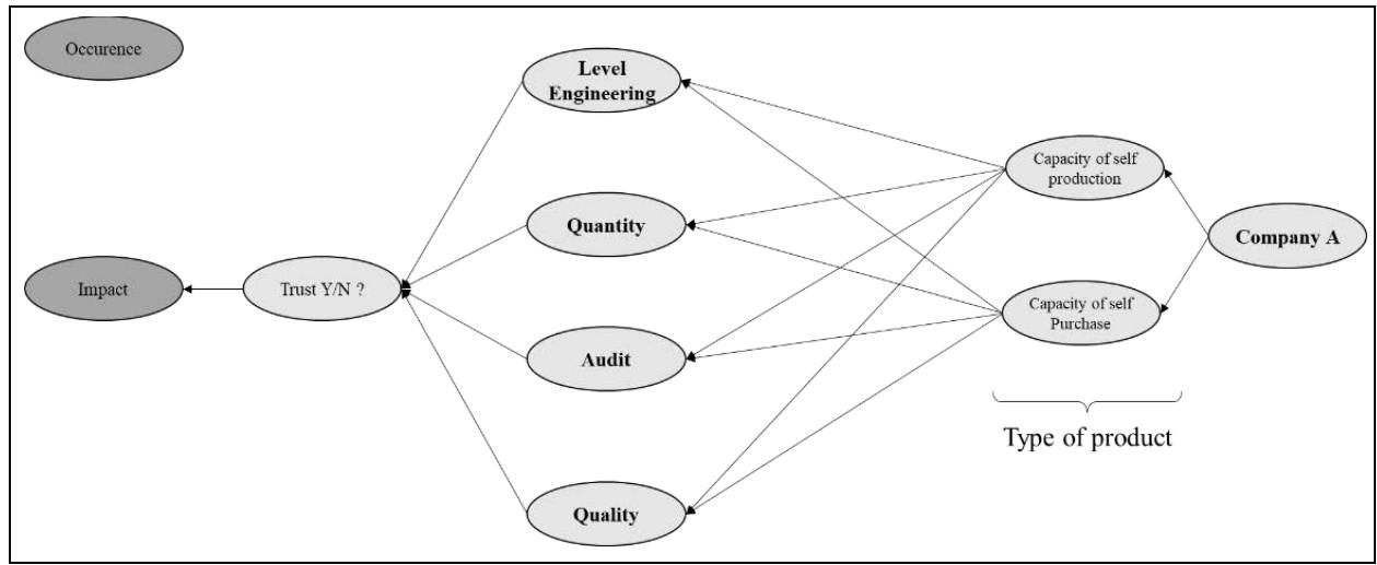Figure 8: Basis Structure of Illustration (By Author) As Naim and Condamin point out (source Operational Risk Modeling in Financial Services by Naim and Condamin), "occurrence modelling is generally the most difficult taks", and it is recommended to follow logic: "The event hits the exposed object during the next period". In other words, the hypothesis of occurrence of the event should only answer the True or False hypothesis. This corresponds to a quantification in yes/no or probable form of the arc. For example, by counting the number of wins or losses over a period of time. By applying a general evaluation that is deductive, inductive and subjective, as we have already specified, we refine the level of occurrences as well as the associated impact dependencies. Impact modeling follows a similar logic since it is quantified to the extent of the impact of Gains or Losses that has already taken place by experience. That is to say that we must quantify in a pragmatic way (we paraphrase Naim and Condamin) at the level of the impact conditions. #### Practically that does Mean Following: - The Impacts are the engineering level, quantity, audit, quality represents the link to impact. - The Quantification is the engineering level, quantity, audit, quality changes with the effort put into the number of iterations to positively change the impact confidence. - The Occurrence: The scenario occurs when engineering level, quantity, audit, quality changes confidence increases. Then we can improve this structure with the structure improved byelicitations and adding values (Figure 9).  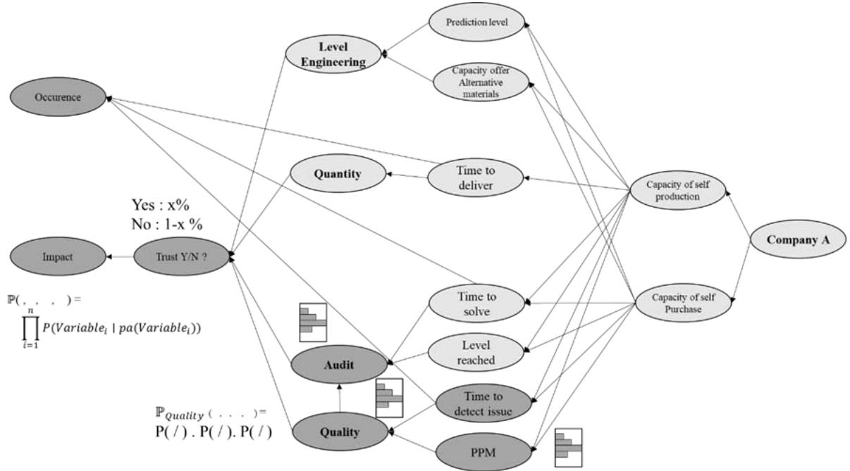Figure 9: Basic Improved Structure (By Author) The organization has legacy of experiences or create expected dependances and can quantify this new link which will require up-front expert judgements. We want to put the scope on the quality-audit branches as an illustration. Adding Values: To improve occurrence scenario, we can add different values like predictions performance to influence the engineering level or time to detect issues for the quality. In the example, the resulting naive Bayesian model will calculate the probability of the target variable corresponding to the Company A, which is the entity under study in the scenario. Trust (Y/N): Indicates the level of confidence of the Quality Criteria during the negotiation given to an entity (Boolean variant) and is a function of the other variables (Production/Purchasing Capacities, Type, etc.): $$ \mathbb {P} _ {\text {Q u a l i t y}} \left(\text {T r u s t} \mid \text {V a r i a b l e s}\right) = P (\text {T r u s t}) \times \prod i P (\text {V a r i a b l e i} \mid \text {T r u s t}) $$ Technically, the CPT construction principle must be used in order to optimize the complete network and build the dependencies. A certain amount of data is necessary and that is based on the firm, and their experts as well as the surrounding data. In the example, the resulting semi-complete Bayesian model will calculate the probability of the network that satisfies the Markov conditions by calculating the network path, i.e., the product of the dependencies of the variables (Variable i) and their parents noted pa(Variable i). $$ \mathbb {P} (T r u s t, V a r i a b l e s, T y p e s, C a p a c i t y, C o m p a n y) = \prod_ {i = 1} ^ {n} P (V a r i a b l e _ {i} \mid p a (V a r i a b l e _ {i})) $$ Thanks to this path, retroactivity, i.e. the ex-Ant pathway, is direct and possible unlike an AHP approach. In addition, an ex-Ant analysis impacts all the elements of dependency and not just one. The reader will probably have noticed that there is a major difference with AHP since we do not apply subjective judgments between dependencies but we rely on logical links, which is much more credible and effective for a dynamic simulation in negotiation. ## IV. SOFTWARE TOOLS RB modelization effort will not be effective without a suitable software support. Many systems commercial exist such as Bayselab, BayesiaLab, Bayes Fusion, Hugin, Netacaor R-based programming tools (Scutari $^{65}$ ) such as: bnlearn, Catnet, deal, pcalg, gRain, Rbmn. After crossing literature analyses (Michiels $^{66}$, Naim $^{67}$ ) and criteria such as general coverage in terms of applications, accessibility, self-autonomy and moderate price, we chose Netica from Norsys Software Corp. Netica is widely used in many case studies (The entry "Netica" & "Case study" gives 2990 results in google Scholar in 2025). The tool is simple thanks to its user-friendly interface and accessible to first-time users as well as experts and covers the majority of the tools needed for analysis. The product facilitates elicitation and inference, which is essential because of the expert origin datas that the agents can use to generate complex cases, which leads to the creation of various scenarios required in complex negotiation. ### a) Validating the Robustness of Bayesian Networks The main objective in Bayesian networks is to continuously update the level of likelihood. This can be achieved by various techniques that we will list here without going into detail. There are two general approaches to making a Bayesian network robust, namely parameter learning and structure learning. - Learning Parameters: where the system is fixed but for which it is necessary to estimate the conditional possibilities of each node of the network, therefore quantitative, which are defined by data as well as that of expert(s). It is divided into three depending on whether the data is Complete, Incomplete and missing data. - Complete Data: When the data are complete, statistical estimation techniques such as likelihood maximization (MV), posterior maximization (MAP), and a priori expectation (EAP) are used. Bayesian IRL, for example, combines MV and MAP with softmax logic to infer reward functions. - Incomplete Data: In the majority of complex cases, the data is incomplete and there are methods such as Estimator-Maximizer (EM), Missing Completely at Random (MCAR), Missing at Random (MAR), and Not Missing at Random (NMAR). These methods, developed by Little & Rubin (1987), are described in the literature by Leray, Naim et al. (2017), and Jouffe and Munteanu. - Noisy Data: When data are scarce but a priori knowledge is available, the principle of elicitation is applied, often associated with a confidence scale and corresponds to expert knowledge. - Learning the Structure: where the system must respond to the best graph to solve the task to be performed hence qualitative and defined by expert(s). Algorithms such as PC (Peter and Clark) and IC (Inductive Causation) are used to identify conditional independence in the data, simplifying the model and making inference more efficient. Criteria like entropy, AIC, and Bayesian scores can be used to evaluate and compare different model structures. Most of these techniques are integrated into Bayesian software: Netica, Bayselab Bayesia Lab, Bayes Fusion, Hugin and Bayserver which is a Bayesian modeling software available online. ### b) Illustration Supported by Software ToolNetica As already mentioned, we propose to focus on one DAG: the quality branches of the network. To build a quantized Bayesian network, each node must be associated with a conditional probability table (CPT) which describes the probability of each possible state of the node based on the dependencies of its parents. To Define Node States, we must identify the possible states of each node. - Occurrence: {Rare, frequently} - Impact: {Low, Medium, High} - Trust: {Yes, No} - PPM (Parts Per Million): {Low, Medium, High} - Detection Time,: {Short, Medium, Long} - Quality: {Good, Medium, Bad} We assume to build the corresponding CPT based on expert information (Figure 10). As we do not have experts around, we have asked Chat_GTP to generate the number in order to avoid to be self-biased by some self-predicting results. Figure 10: CPT of Illustration (By Author) <table><tr><td colspan="5">Occurrence</td><td colspan="4">Time_of_detector</td><td colspan="4">Impact</td><td colspan="3">Quality</td></tr><tr><td>Company A</td><td>Trust Y/N</td><td>Rare</td><td>Frequently</td><td>Quality</td><td>Short</td><td>Long</td><td>Medium</td><td>PPM</td><td>Low</td><td>Medium</td><td>Strong</td><td>Audit</td><td>Good</td><td>Medium</td><td>Bad</td></tr><tr><td>Capable</td><td>Yes</td><td>0.90</td><td>0.10</td><td>Good</td><td>0.70</td><td>0.20</td><td>0.10</td><td>Low</td><td>0.80</td><td>0.15</td><td>0.05</td><td>Yes</td><td>0.85</td><td>0.10</td><td>0.05</td></tr><tr><td>Capable</td><td>Yes</td><td>0.90</td><td>0.10</td><td>Medium</td><td>0.30</td><td>0.50</td><td>0.20</td><td>Medium</td><td>0.60</td><td>0.30</td><td>0.10</td><td></td><td></td><td></td><td></td></tr><tr><td>Capable</td><td>Yes</td><td>0.90</td><td>0.10</td><td>Bad</td><td>0.10</td><td>0.30</td><td>0.60</td><td>High</td><td>0.40</td><td>0.35</td><td>0.25</td><td></td><td></td><td></td><td></td></tr><tr><td>Capable</td><td>No</td><td>0.70</td><td>0.30</td><td>Good</td><td>0.50</td><td>0.30</td><td>0.20</td><td></td><td></td><td></td><td></td><td>Yes</td><td>0.70</td><td>0.20</td><td>0.10</td></tr><tr><td>Incapable</td><td>Yes</td><td>0.40</td><td>0.60</td><td></td><td></td><td></td><td></td><td></td><td></td><td></td><td></td><td></td><td></td><td></td><td></td></tr><tr><td>Incapable</td><td>No</td><td>0.20</td><td>0.80</td><td>Medium</td><td>0.20</td><td>0.40</td><td>0.40</td><td>Low</td><td>0.50</td><td>0.40</td><td>0.10</td><td></td><td></td><td></td><td></td></tr><tr><td>Incapable</td><td>No</td><td>0.20</td><td>0.80</td><td>Bad</td><td>0.05</td><td>0.20</td><td>0.75</td><td>Medium</td><td>0.30</td><td>0.50</td><td>0.20</td><td>No</td><td>0.30</td><td>0.40</td><td>0.30</td></tr><tr><td>Incapable</td><td>No</td><td>0.20</td><td>0.80</td><td>Bad</td><td>0.05</td><td>0.20</td><td>0.75</td><td>High</td><td>0.10</td><td>0.40</td><td>0.50</td><td>No</td><td>0.30</td><td>0.40</td><td>0.30</td></tr></table> As you can see, the CPT only contains a certain amount of information that we have left free so that the system is able to extract new knowledge: we use Netcha from Nordsys © for our simulation. Taking the learning function that is based on a CPT that we have firstly entered in an Excel file, Netica will execute the corresponding Bayesian network and the researcher will create the links to obtain the corresponding DAG below(Figure 11).  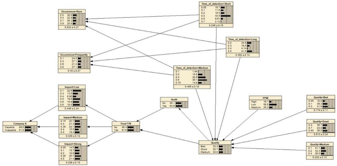Figure 1: DAG of Quality structure underNetica® (By Author) ### c) Simplification of the Nodes As already mentioned, the number of connections clime rapidly and there is a necessity of reduction, otherwise the number of parent links with eventually to much entries and generate to much variables and lead to overlearning and overprocessing. This action is difficult but necessary. On the illustration (Figure 12) we can report a randomization of the new model with better Capability Output [35.1%/ 64.9%] against the previous model [49% / 51%].  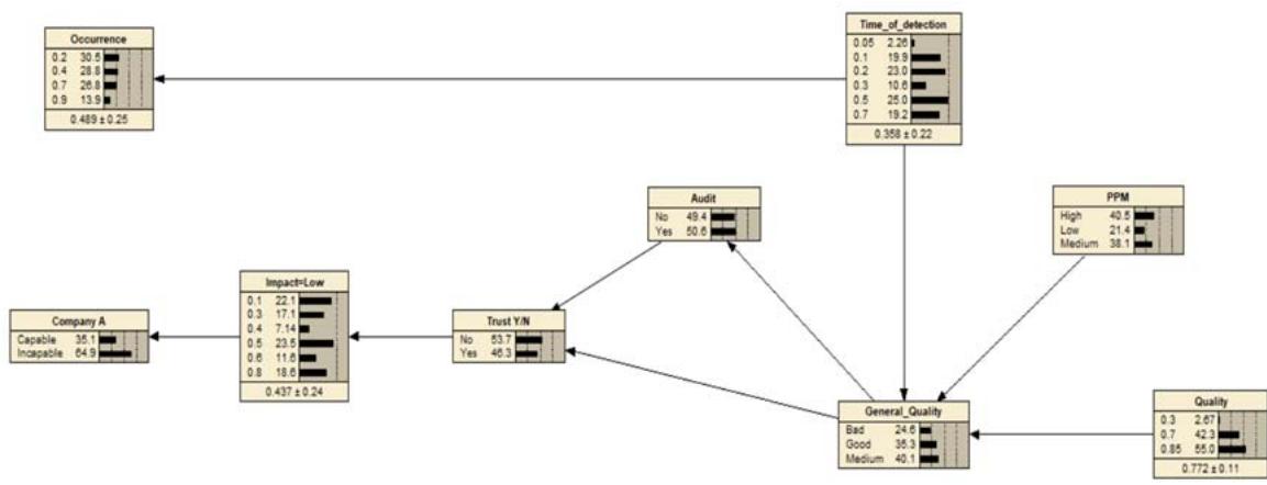Figure 12: DAG of Quality Improved Structure under Netica® (By Author) Since this is a case study, we would like to remind the reader that it is of course necessary to confirm with the expert elicitation and validate the principle in each specific organization on each specific case (product, market i.e) ### d) Extended Perspective and Operational Deployment There is a novelty in this work because we can predict the behavior of the price in a negotiation by applying a hybrid Bayesian network method. First, by establishing a set of variables to construct a Bayesian network in order to obtain a final conditional dependency in order to obtain an impact and an occurrence of the scenario studied and where: 1. Impact (li): Discrete variable with possible values {low, medium, high}. 2. Occurrence (Oi): A discrete variable with possible values {rare, frequent}. 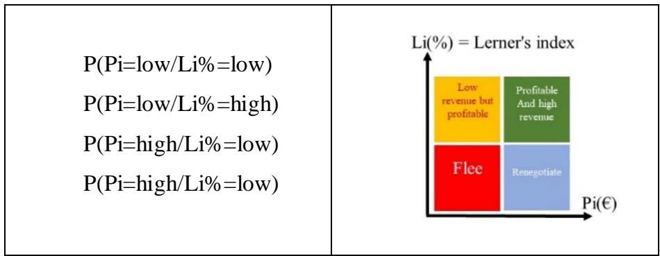Then, considering during the negotiation the prices Pi (€) are proposed with a correlation of the Lerner index Li (%) in order to categorize the following (Figure 13) four cases:  Figure 13: Lerner/Pi Matrix The price Pi (€) itself is given by the negotiation that the seller manages with his customer, but Li (%) is influenced by the total cost CTi (€) and the price Pi (€), i.e. the extra and intra-organization. Consequently, we can establish a correlation between the price, the Lerner index and Pi (\%) and therefore Oi (\%) and li (\%) in the following way (Figure 14): Thanks to these links, the work of the Experts can start in a coordinated way. Thus, to return to the example. Lerner Index is moreover semi-empirical because MC is fixed and the price is variabilized by an observation variable. If we take the Lerner index as an observation variable that the selling agent can use, it represents for him a good indicator of the performance of a deal a priori. In a Bayesian update, it corresponds to the likelihood in the Bayesian theorem. Thus, either: - The price (P) is a direct observation. - The marginal cost (MC) is a latent variable estimated and subject to the variability of indices and can be updated via Bayesian learning. - The set (L) influences the actualization of the strategies. - Index (I) calibrated to costs Marginal (MC) with respect to the number of times that if the marginal cost exceeds a certain level due to material effects, the compensation will be adjusted to the price (P) The index corresponds to an a priori law that is adjusted to the likelihood, for example, that the customer is not in a position to take a risk: Law a Posteriori $\propto$ Law a Priori $\star$ Probability Risk index/Profit Lerner Index Price/Risk index Bayesian logic allows this counterintuitive approach which, as in the example, will allow both the selling agent and the buying agent to adjust the level of the Index (I), the frequency of the number of occurrences of times when the index will exceed a certain level without this impacting either the seller or the buyer. The Lerner index is a reference -or a priori law-associated with the measurement of impact and occurrence since they together represent an indicator of the performance of the structure. In the case of a high impact in terms of profit associated with a high occurrence represents a favorable case. On the other hand, if the Lerner index meets the objectives, corresponding to a high impact but associated with a low occurrence, the structure can be corrected with much more precision in order to correct the occurrence. It should be noted that with the increasing performance of LLMs (GTP-4 $^{68}$, Llama $^{69}$ ) which are more and more capable of complex and subtle reasoning, the evaluation of Occurrence and Impact can be helped by Als that will allow questions to be asked and cross-referenced. Thus, like Virginia Tech's Crowldea $^{70}$, which is a software platform that reveals meaning without supervision in order to reveal reasoning processes, multi-agents will confront evidence of factualities justifying conclusions to avoid human biases of over or under interpretation. As a result, Bayesian networks are generally able to assess both impact and occurrence, which in some specific cases can present challenges that require continuous updating of learning by experts, elicitation, learning tests and reduction in the number of links that can lead to super-computation. Thanks to inference, the PWT,VBP team will be able to retroactively (ex Post) correct li (%) and Oi (%) by adding other variables to the Bayesian network in order to optimize Pi (%) and refine Pi (€) Thus, in the DAG Client example, despite frequent detection of quality cases and despite the client's trust thanks to a positive audit, there is a strong possibility that the organization will be judged incompetent because despite the good qualitative focus, the organization could not be judged to be sufficiently responsive in cases of problem solving. Therefore, in the broader context of vertical production, a high level of quality assurance of its suppliers must be maintained if the integration rate is low. In general, extending the level of quality in correlation with the vertical integration of self-produced or purchased components will have an impact. This is nothing new, one might say, but the algorithm shows the logical links that lead to such an impact. $$ P \left(P i = \left\{ \begin{array}{c} H i g h \\ M e d i u m \\ L o w \end{array} \right.\right) = \sum_{I i, O i} P \left(\left(P i = \left\{ \begin{array}{c} H i g h \\ M e d i u m \\ L o w \end{array} \right.\right) / I i, O i\right) P (I i) P (O i) $$ However, it is necessary to ensure a good correlation between price and gross margin accurate information which means that the data must be mastered by the experts PWT, VBP by integrating high, medium, low margins according to the variability of exchange rates, material costs, labor costs, energy costs. This requires precise work upstream or can be the subject of a framework by elicitation. By The Quality DAG is one of the many scenarios. In order to obtain the impact and occurrence of the complete network, it is therefore necessary to build all the DAG scenarios. ### e) Operational Deployment During the negotiation, the propagation of beliefs, via a more general inference, which is automatically calculated in software such as Netica, makes it possible to obtain up-to-date results useful to the PWT, VBP teams based on the work of the sales team and reinforces the learning phenomenon of the system. This structured and logical approach makes it possible to analyze and anticipate price behavior in a negotiation using a hybrid Bayesian network thanks to a set of discrete variables while remaining unclear in some cases to evaluate the impact (li) and occurrence (Oi). Using the Lerner index to categorize the prices in four cases, we relate the proposed price Pi to the gross margins (Li), also incorporating the impact of the total cost CT. This allows pricing and margin strategies to be defined under specific conditions, which is therefore particularly useful in the complex negotiations that the seller has to conduct. Ex post feedback through inference to correct li (%) and Oi (%) allows to adjust the probabilities and correlations in the Bayesian network with new information that will be provided by the whole group as well as the flying agents, making the model more robust and responsive to changes in the context of the negotiation. The use of Netica integrates Inference which makes it possible to automate the propagation of beliefs because it simplifies the complex calculations associated with Bayesian networks. This allows a dynamic update of conditional probabilities as new information emerges during the negotiation. The result is a marginal probability. To obtain the marginal probability $P(\mathsf{Pi} = \{\mathsf{High}; \mathsf{Medium}; \mathsf{Low}\})$ of each single PI case it is necessary to calculate the distribution. That mean calculate the sum products of the conditional probabilities and marginal probabilities of the parent variables: incorporating margins adjusted for exchange rate fluctuations, raw material, labour and energy costs, greater accuracy is added to the model. This type of upstream work allows price estimates to be better framed according to cost variability. Indeed, the elicitation framework of the expert group is a good option for managing vagueness, especially when it is difficult to quantify certain elements or to accurately predict cost variations. This approach makes it possible to capture expert knowledge, thus facilitating a more realistic and nuanced Bayesian modeling in the context of the negotiation. Our approach reinforces the robustness of the PWT-VBP_negociation model and limits uncertainties in the evaluation of scenarios while being realistic about the reality of unknown data, and requires a group of the pricing teams (PWT, VBP) and Sales Force assisted by experts corresponding to certain DAGs (Engineering, Quality, Production,...). In the realm of the unknown, BN represents a breakthrough in a priori, unknown relationships between data and promising approach. For use in the complex, the advantage of Bayesian networks is the causal representation in the form of directed causal graphs. In the factual and counter-factual logic, consequently (according to... Naim...) BN are better suited to predict, diagnose, control, simulate behavior and analyze system data and ultimately make decisions about the system. The search for values is a complex field and responds to the same problems in which Bayesian networks can make a difference. In this sense, there are no fixed parameters to be placed in a Bayesian network, but a priori unknown links to detect common values in a pricing system, since the elicitation will be built as the system is built, which is based on a dialogue between buyer and seller. ### f) Training Mastering BN requires a set of prior understanding and training such as being accustomed to basic probability concepts and Bayesian logic but also Behaviorist logic and Prospect Theory in order to help agents understand the underlying principles of the decision and not make biased interpretation errors. The training consists of theoretical training followed by a set of illustrations around case studies where Bayesian networks have been used to model complex decision-making processes through the use of visualization tools in order to understand belief updates. Finally, it will also consist of creating concrete interactive simulations where users can observe the impact of the data collected on the posteriori probabilities and developing analysis tools that facilitate the collection and integration of relevant by providing intuitive user interfaces. The complete course will consist in three days in accordance with what is recommended by the Bayseialab firm[^71](See more in some cases). By offering these training courses to the PWT and Values functions, agents can work on common cases in order to strengthen their cohesion around the dialogue and opposing difficulties that agents encounter on a daily basis. ## V. RECOMMENDATIONS We presented an extended deployment tool in PWT and VBP by strengthening the PWT-Sales Force expertise. In opposite to most MDCM, Bayesian is data and subjective driven in order to reflect rational and rational limited human organization behaviors and improve decisions. At this stage, our research is theoretical and requires experimental verification to be fully validated. However, experiments are ongoing to be tested in Vitro and in Vivo and the results will be reported in following publications. ## VI. CONCLUSION The purpose of this article was to highlight that in PTW, Bayesian can be call to help solve the scope of Values in complex B2B, B2G selling negotiation process. The AHP Fuzzy is a tool which helps negotiations in B2B but has the disadvantage to be relatively static and not enough fitted for negotiations. According our research a combination of AHP and Bayesien is rare and was only applied according us in marketing research framework but not negotiation. Papic-Blagojevic and All[^72] propose to use Bayesian networks to establish the links of dependencies between tourists, and use the strongest dependencies obtained in order to classify tourists satisfaction with AHP. From a methodological point of view, the Bayesian network is used in a way prior to AHP. By applying the best dependencies, the Bayesian Network is therefore able to establish a preferential structure which in opposition a Postulate methodology would have difficulty producing in fact the treatment of uncertainty. Bayesian Network overcomes complexity and uncertainty in complex selling. BNs are part of the cohort of artificial intelligences but they must be trained. BNs are tools that connect field experts and analysts to solve problems (Naim)[^73] in order to train a system that will improve. Taking into account the uncertainty, the Bayesian network is able to generate scenarios that are very useful in a negotiation, as they are for detecting terrorist risks (Naim-Chapter 14) per example which both are two unlikely unpredictable fields. Zeng and Sycara[^74] show also the benefit of learning in the framework of a sequential negotiation model through the process of updating Bayesian beliefs. We cannot hide the main challenge around the fact that the real cause of a consequence is often complex to determine and will influence effectiveness of BN. In fact, the deployment of BNs is similar to that of VBP which request similar attentions. They complement each other but require time and champions (CEOs) to bring them within the organization in order to form "Superforecaster" Experts Team (2016)[^75]; 2024[^76]) which are individuals with characteristics capable of making exceptionally accurate predictions and very useful for complex predictions combined with the B2B negotiation framework. Through this article, we want to convince company champions to systematize their organization by taking into account uncertainty with help of Bayesian deployment in PWT in order to generate elicitation, think toughly about the deterministic/indeterministic which will improve the methodology of knowledge their markets, their customers and obtain better Valued results by increased leadership. The contribution of Bayesian networks to the organization can be used as a Knowledge Tool focuses on a structural logic of the offer so that it can be adapted synchronously and asynchronously with flexibility to the customer. The power of our proposal is therefore mainly to be a complementary tool to the commercial and program function in order to prepare the negotiations and the possible alternatives by taking into account human behaviors to adjust the best price and the best values during the consultation phase and which can be adjusted after elicitation to the negotiations. The time phases are: Pre Inference< Pre Decision <Inference <Elicitation <Arguments Consequently, once the conditions for understanding the variables have been well mastered, the frequency of updating is that linked to the frequency of updating the consultation program and which should be built up over a few weeks if we stick to a personal empiricism of the automotive sector, for example. The method is perhaps more suitable for consultation phases and we propose the deployment as follows in a B2B deployment: <table><tr><td>Phase</td><td>Deployment</td><td>Source data</td><td>Building the model</td><td>Tempo</td></tr><tr><td>RFQ or RFI</td><td>Preparing the model</td><td>Customer Package CoC Data</td><td>Pre-Inference by Basic Model Construction</td><td>1 week</td></tr><tr><td>Phase 0</td><td>Basis for the decision</td><td>Décision de consultation</td><td>Utilisation du modèle de base pour participer à la décision GO/NO-GO</td><td>1 day</td></tr><tr><td>Phase 1</td><td>Deploying the model hardened with internal data: Costs</td><td>Response to consultation</td><td>Complete inference based on customer contacts, CoC, and internal elicitation</td><td>2-4 weeks</td></tr><tr><td>Phase 2</td><td>Structuring arguments to strengthen the negotiation</td><td>Submission of the offer</td><td>Elicitation</td><td rowspan="2">4-12 weeks</td></tr><tr><td>Phase 3</td><td>Leason Learn Contract Structuring/Learning Support</td><td>Acceptance/R ejection of Offer</td><td>Technical and commercial arguments</td></tr></table> Funding Declaration and Conflict of Interest Declaration This research did not receive any specific grant from funding public agencies, software company, commercial, or none-profit sectors. The authors declare also no financial interests or personal relationships that could have appeared to influence the work reported in this paper. ### Overview and Purpose In Pricing, Value Base Pricing (VBP) in B2B industry is a proven profit generator according Hinterhuber, Liozu. The literature also highlights that VBP does not benefit a cooperative equilibration between buyer and seller. In this article, we propose a new methodology for resolving Value Base Pricing deployment, which is captured by the customer in the majority of cases during the commercial negotiation. There are pricing methodologies which do not all operate in the same timeframe in accordance with a negotiation and are therefore not suitable for commercial purposes. Among all the methodologies, the Price Wining Target (PWT) is an active method that does not advocate a target price but an optimal price in ex-Ant correction of ex-Post decisions needed in negotiation cases. PWT relies on decision-making models in limited rationality (H. Simon). As well among all the decision models, Bayesian Model is a robust mathematical framework which manage uncertainty in complex decisions frames. We propose to link the PWT to Bayesian logic. The integration of PWT in Bayesian Network based model create a bridge between the game theory and practical applications of zero-sum games, non-zero-sum games as well as cooperative games. Bayesian Network has already proven itself adding value in multiple domains of Financial and Banking Risk Management, Credit Rating risk, Medical Diagnosis, Complex Genetic modelling, Artificial Intelligence in beliefs updating under uncertainty, Enhancement Cognition, among others and this contribution propose to deploy it in the Pricing organization. We deploy theoretically and practically a methodology based on the mathematical-Bayesian Modeling software Netica. Then we show how theoretically expert of pricing and commercial resources available in organizations can be linked through the model. In order to improve values predictability the connection of Bayesian and PWT model to group of experts, organization will be able to build a large number of scenarios reflecting the complexity and dynamics of real situations of symmetrical, dissymmetrical frameworks useful to optimize dynamic negotiation in B2B business relationships.

Generating HTML Viewer...