I. INTRODUCTION

The Dual Thrust Solid Rocket Motors (DTSRMs) are solid propellant rocket motors that have the capability of yielding a dual (step) thrust; a high thrust followed by a lower one. This boost-sustain feature finds applications in a variety of guided missiles. Boosting the missile allows it to swiftly accelerate to the nominal flight speed in a minimum uncontrolled flight time. The subsequent low thrust ensures near-zero acceleration to maintain the nominal flight speed (proper for control) for a maximum controlled flight time.

A dual thrust is achieved by different motor designs including single-chamber and single fixed nozzle, single-chamber and single variable nozzle, double-tandem chamber and single external nozzle, double-chamber and double nozzle configurations. Nonetheless, the simplest design is the one in which one chamber incorporating two grains of different configurations is used. This simplicity comes with motor operation complexity as it involves five different phases including two steady-state phases and three transient phases (ignition, transition, and tail-off).

Understanding the SPRM operation is a crucial step in missile mission design. Experimental measurements of chamber pressures and motor thrust are perhaps the most reliable in defining the overall motor operation. Nevertheless, practice shows that variable thrust measurement of DTSRM may be troublesome due to variation in thrust level. While measuring pressure can be simply achieved, the use of two different load cells for the same motor may not be as simple. Analytical techniques based on solving internal ballistic relations may also be used to estimate the motor pressure and thrust. However, if it is sought to understand the flow behavior and explore its features along the motor, neither experimentation nor analytical technique is the right approach. Numerical simulation of the flow along the DTSRM gives a better understanding of the multiple flow features associated with the two levels of pressure including streamlines, pressure, temperature, density, and velocity variation along the motor which cannot be attained from experimental measurements or analytical calculations. In addition, both numerical simulations and analytical calculations have the advantages of higher flexibility and lower cost and risk compared with experimental measurements. Yet, numerical simulations have higher fidelity compared with analytic calculations. One key aspect of the successful simulation is the proper definition of operating and boundary conditions. Using accurate experiment-based inputs would indeed yield more reliable simulation results.

The use of numerical simulation via the computational fluid dynamics (CFD) approach to understand and analyze the flow field through solid-propellant rocket motors has been widely adopted [1-8]. Some researchers focused on the ignition transient phase [9-15] to investigate phenomena accompanied by starting transient such as internal flow chocking, preignition chamber dynamics, and boundary layer displacement. While some focused on quasi-steadystate and tail-off phases [16] to analyze the validity of performance prediction for parameters such as pressure, thrust, and nozzle throat variation. Pressure oscillation and acoustic instability taking place in the solid rocket were also addressed using numerical simulation [17-21]. Recently, more attention has been paid to using CFD in simulating solid rocket motors regression [22]. Li et al.

[23]presented an integrated framework for coupled simulation of internal fluid flow in a solid rocket motor and burning surface regression of propellant. Lin[24]developed an immersed boundary method to avoid the cumbersome re-meshing for simulating the coupling of gas flow and burning surface regression in solid rocket motors. Zou et al.[25]developed a numerical model to investigate the regression rate and the combustion process of a combined solid rocket motor for different grain inner diameters. Some advanced topics related to numerical simulation for solid rocket motors have been discussed. Han and Kim[26]examined the interaction between burning module, structure, and fluid inside solid rocket motors. Hemanth and Jyothi[27]simulated the flow inside a retro solid-propellant rocket motor.

The objective of the present work is to simulate the flow inside a DTSRM using computational fluid dynamics based on the pressure from experimental measurements to reflect the internal flow characteristics for the combustion chamber and nozzle together. The grain recession calculation was carried out to obtain the grain shapes along the whole motor burning time which represents the computational domain used in simulations. The simulations will cover the whole burning time starting from ignition to tail-off obtaining all possible internal flow parameters. From these parameters, the internal ballistics of the case study DTSRM and the resulting thrust is calculated. In such cases, simulation results may be used to predict motor thrust with accuracy closer to experimental measurements compared with the analytical calculations.

II. EXPERIMENTAL MOTOR

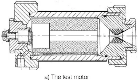
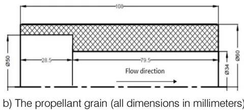
For the present case study, a test solid rocket motor is adopted, Figure 1a with the pressure transducer adjusted at the head end of the motor. A tubular grain of two different inner diameters along the axis is used. The tubular grain is inhibited from the outer surface adjacent to the motor casing while it is allowed to burn from all other surfaces, Figure 1b. The solid propellant composition includes ammonium perchlorate, Aluminum powder, and HTPB with the percentages shown in Table 1. The burning law for the propellant is defined as:

	AP	AI	HTPB
Chemical formula	NH4ClO4	Al	C7.09H10.86O0.227
Weight percentage[%]	69	17	14
Enthalpy [kcal/mol]	-70.69	0	-14.64

III. METHODOLOGY

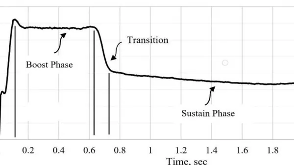
For sake of numerical simulation, the pressure $\sim$ time curve from experimental measurements was divided into five regimes namely, ignition transient phase, boost steady phase, transition transient phase, sustain steady phase, and tail-off transient phase as shown in Figure 2. For each of the two steady-state phases, four-time instances are investigated; one at the start, one at the end, and two in the middle of each phase. In contrast, the full duration of each of the three transient phases is examined. The grain recission is calculated at each burning step for the whole burning time to be used in simulations representing the three transient phases and the eight points of steady-state phases computational domains.

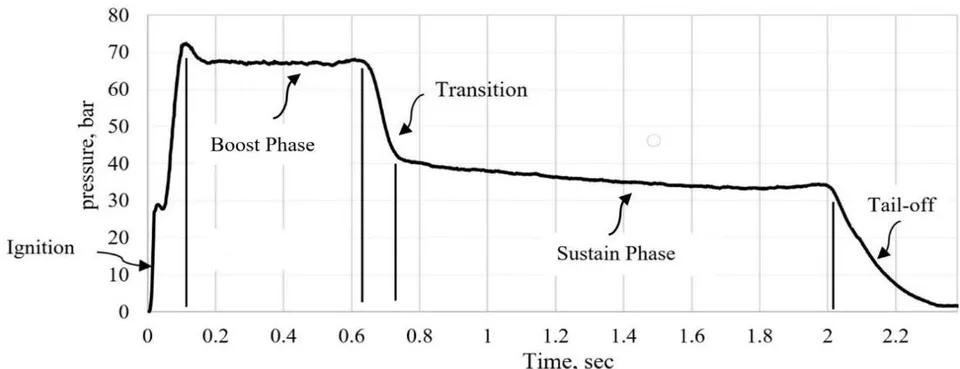
The ignition phase represents the rise of the pressure from 0 to 71 bar in about 0.1 seconds, the boost phase of the test motor operation endures for about 0.5 seconds where pressure varies from about 71 to 68 bar. The transition represents the change from boost to sustain phase with a variation of pressure from 68 to 42 bar in 0.1 seconds. During the 1.12 seconds sustain phase, the motor pressure drops from 41 to 36 bar. Finally, the tail-off phase represents the collapse of pressure from 36 to 1 bar in about 0.33 seconds. The burning of propellant grain surfaces results in gases with direction normal to these surfaces, to simplify the problem, and as the pressure transducer is adjusted at the head end of the experimental motor, the simulation input (experimental pressure measurements) is adopted as pressure inlet.

a) Computational Domain

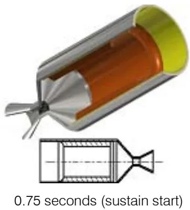
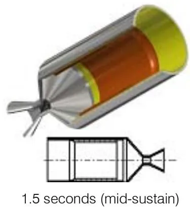
Due to grain regression during both boost and sustain phases, the computational domain geometry varies with time. Figure 3 shows the instantaneous grain locationscalculated using the burning law (Equation 1) based on instantaneous chamber pressure values at five different times of burning. For more realistic simulations, the natural change of sharp corners into rounded ones upon regression is taken into consideration. The grain configuration at 0 seconds represents the computational domain for ignition phase transient simulation and boost start steady-state simulation. Grain location at 0.6 seconds represents the domain for boost-end steady-state simulation. Grain location at 0.75 seconds represents the domain for both sustain-start steady-state simulation and boost-sustain transition simulation. Grain location at 1.5 seconds is taken to define sustain-end steady-state simulation. For tail-off transient simulation, an empty chamber is considered.

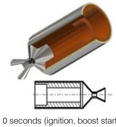
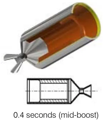
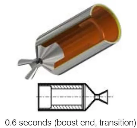
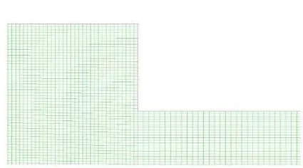
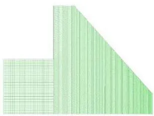
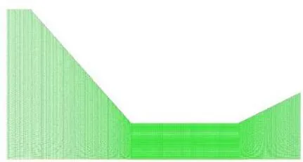
Due to the symmetry of flow and domain, two-dimensional axisymmetric computational domains are developed for all simulations. Multi-block structured grids are constructed such that grid quality is increased at areas of interest namely, solid walls, the nozzle critical section, and its upstream and downstream vicinity.

The mesh in the present work used structured grid element shape with appropriate number of divisions that suit each part of the motor. Spatial resolution is assessed through a grid independence check, the pressure at the throat was observed, and the grid-independent solution was obtained at 252000 cells. All wall boundaries in the domain are defined with the noslip condition while the lower (bottom) boundary is defined as the axis. Consistent with experiments, the downstream (right) end of the domain is defined as a pressure outlet with atmospheric pressure definition. To simplify simulations, and since the pressure input to simulations is based on readings of a pressure transducer that is adjusted at the head end of the experimental motor, the upstream (left) end of the domain is defined as a pressure inlet as shown in Figure 5, which illustrate the mesh used in boost start steady case.

(a)

(b)

(c) Figure 5: Mesh used in the boost start phase

b) Boundary Conditions

For the steady-state simulation, four main cases were selected to be discussed (boost-start, boost-end, sustain-start, and sustain-end), the instantaneous combustion pressures at the time instances in concern are set based on Figure 2. Hence, four steady cases correspond to inlet pressures of 71, 68, 41, and 36, respectively will be explained in detail in the current study. Another four cases are simulated, two in each steady phase to cover more points in the thrust curve and increase the prediction accuracy.

For transient phases simulations of Transition and Tail off, pressure inlet values are user-defined functions of time extracted from Fitted trendlines equations of the experimental curves illustrated in Figure 6, whereas in the ignition phase, the pressure-time relation is input as a table of discrete points (extracted from ignition experimental curve) within which instantaneous pressure value is interpolated.

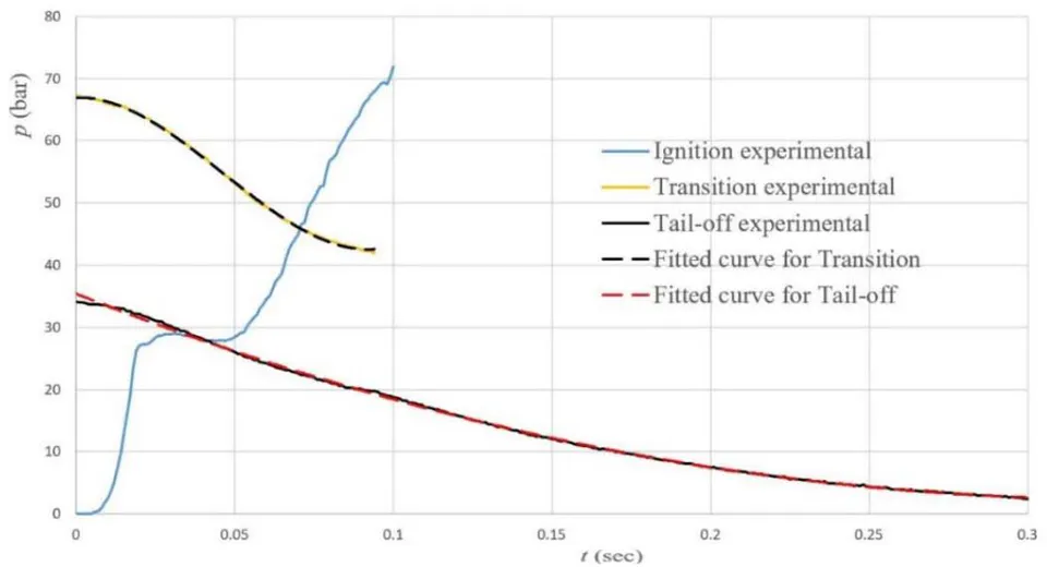
For boost-sustain and tail-off transient phases' simulations, the experimental pressure-time curve data is analyzed and equations of the fitted curves (polynomial equations of trendlines) are used in the user-defined function input files. These functions are:

Transition phase: $p=64830t^3-9029.6t^2+16.745t+66.935$ (2)

Tail-off phase: $p=303.9t^2-200.28t+35.408$ (3) where $p$ is the inlet pressure value in bar while $t$ represents the time in seconds.

c) Operating Fluid Properties

Properties of working gas adopted in CFD solver setup are sought to be as close to real combustion as possible. This is done by conducting thermochemical calculations using NASA CEA [28] code. It is one of the thermochemical programs that are capable of calculating the chemical equilibrium compositions of a chemical system via minimization of free energy formulation, which allows one to calculate theoretical thermochemical properties. Combustion pressure is input as well as ingredients of solid propellant (listed in Table 1) as reactants in the form of weight percentage along with enthalpy, temperature, and chemical formula of each. Grain burning is considered a finite area combustion problem with a contraction ratio (ratio of finite chamber area to throat area) of 7.475 and an initial chamber temperature guess of 3800k. Table 2 lists the operating gas properties for all steady cases in boost and sustain phases.

Simulation Case Parameter	Boost start	Boost end	Sustain start	Sustain end
Camber pressure (bar)	71	68	41	36
Temperature (K)	3388	3385	3344	3332
Density (kg/m3)	6.9038	6.6119	3.9767	3.4868
Specific heat (J/kg.K)	3547.3	3568.7	3836.2	3910.1
Thermal conductivity (w/m.K)	1.0381	1.0467	1.1554	1.1856
Viscosity (kg/m.s)	9.88 e-05	9.87e-05	9.7925e-05	9.769e-05
Specific heat ratio	1.1411	1.1409	1.1378	1.1370
Specific gas constant (J/K.mol)	323.27	323.397	324.78	325.15

d) CFD Solver Setup

The pressure-based solver for Navier-Stokes equations is adopted. For the pressure-velocity-coupling scheme, the pressure-based coupled algorithm is chosen as it gives a more efficient, accurate, and robust single-phase implementation in cases of steady-state flows. Turbulence is modeled in Reynolds-Averaged Navier-Stokes (RANS) through the standard $k-\epsilon$ model. It is preferred because of its reasonable accuracy and reliability for a wide range of turbulent flows and heat transfer. It is thus the most commonly used turbulence model, especially with solid rocket motors cases [29-33]. Gradients are computed in the current work using the Least-square cell-based method while the PRESTO discretization scheme is chosen as it is more suitable for multiphase simulations. For unsteady simulation cases, the time step size in each case is chosen to be compatible with the input file data based on a temporal resolution sensitivity check. The working fluid is chosen as an ideal gas with the specifications tabulated in Table 2.

IV. DISCUSSION OF INTERNAL BALLISTICS SIMULATION RESULTS

Results of numerical simulation for the flow inside the test motor in concern are discussed below in two sections, transient phases, and steady-state phases.

a) Transient Phases

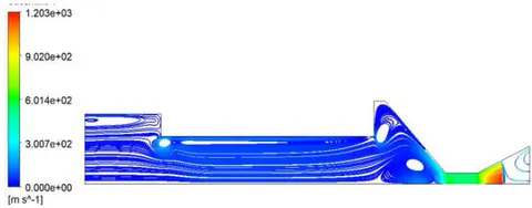
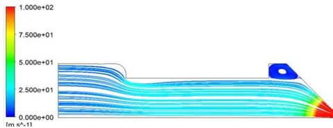
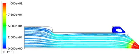
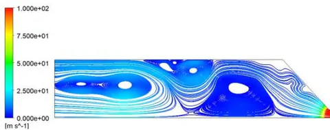
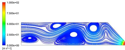
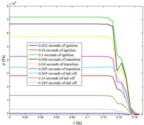
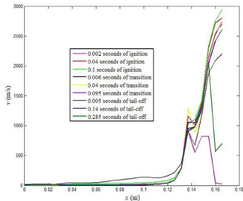
Figure 7 (a, b, c, and d) shows the flow velocity streamlines along the motor at different times of the ignition phase colored according to velocity values, Figure 6.a shows the whole motor with nozzle, whereas the other figures focus on the velocity streamlines variation inside the combustion chamber. Vortices can be noticed inside the combustion chamber at the beginning of ignition, especially in the gap between grain and nozzle. These vortices seem to diminish or vanish with time as the pressure becomes high enough to make the flow smoother. The flow parameters change along the motor at different times of ignition are shown in Figure 8 where flow pressure and velocity along the axis are displayed. Flow pressure has a high, nearly constant, value inside the combustion chamber and these values decrease along the nozzle at all times of ignition. In contrast, velocity is nearly zero inside the chamber and then increases along with the nozzle. It can be noticed that the flow doesn't fully expand along the nozzle at the beginning of ignition where the pressure value inside the combustion chamber is still not high enough.

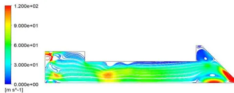
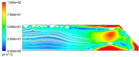
During the transition phase, the pressure drops sharply while the grain almost maintains its configuration. The velocity streamlines variation at different times of transition phase time is shown in Figure 7 (e, f, g, and h). It can be noticed that the flow streamlines as it transfers from the boost phase with high pressure to the sustain phase with lower pressure become smoother. The recirculation bubbles along the motor diminish in number and size. The flow parameters along the motor at different times of this phase are shown in Figure 8. Pressure has a higher value inside the combustion chamber and decreases along the nozzle at all times of burning. The flow velocity inside the

combustion chamber has a low value that increases along the nozzle.

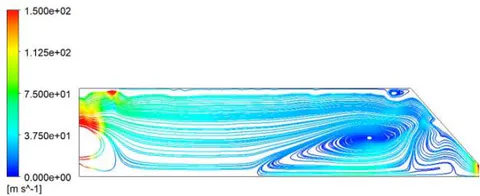
The tail-off phase represents about 0.3 seconds of motor operation. Figure 7 (i, j, k, and l) shows the variation of flow streamlines colored according to velocity values. Over time, the velocity decrease as the pressure inside the combustion chamber is relieved and the streamlines vortices still exist inside the empty motor. The flow parameters along with the motor at different times of this phase are shown in Figure 8.

(a) 0.002 seconds of ignition

(b) 0.006 seconds of ignition

(c) 0.04 seconds of ignition

(d) 0.1 seconds of ignition

(e) 0.006 seconds of transition

(f) 0.017 seconds of transition

(g) 0.04 seconds of transition

(h) 0.095 seconds of transition

(i) 0.005 seconds of tail-off

(j) 0.02 seconds of tail-off

(k) 0.14 seconds of tail-off

(I) 0.285 seconds of tail-off

(c) Velocity Figure 8: Variation of Pressure (left side) and Velocity (right side) along the motor axis at different times of the transient phases

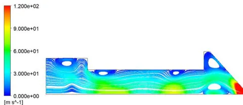
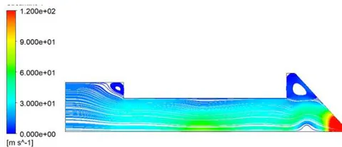
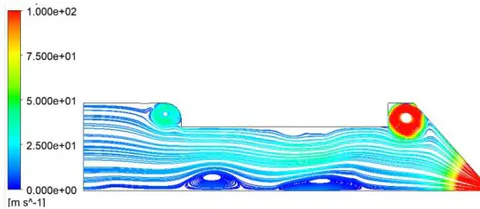
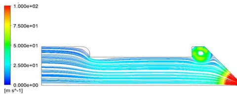
b) Steady State Cases

Four steady-state simulation cases are considered for each phase, the simulation results are presented in detail for two cases at each phase namely; at its start and end. Figure 9 illustrates pressure contours along with the motor for two cases in the boost phase and two cases in the sustain phase. The first case includes the whole motor, while the other three cases focus on the combustion chamber as the pressure values are higher inside it. The pressure clouds concentrate in the middle of the motor and close to the convergent part, the pressure values are higher in the center of these clouds. In addition, the variation of gases pressure and Mach Number along the motor axis at the start and end of each steady phase is illustrated in Figure 10.

(a) Boost start

(b) Boost end

(c) Sustain start

(d) Sustain end

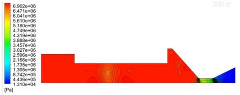
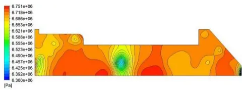
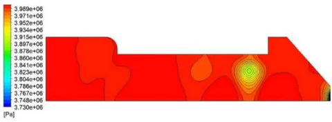
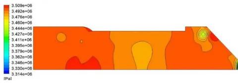
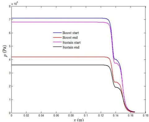
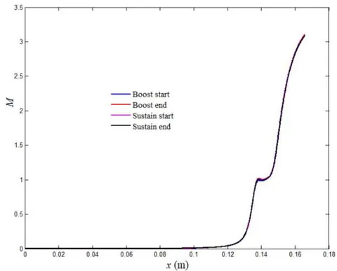
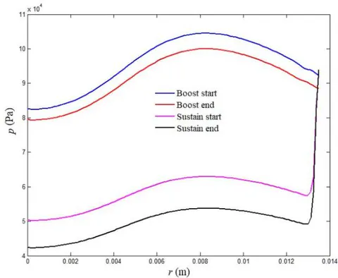
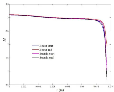
The pressure at the combustion chamber is high and starts to decrease once it enters the nozzle and continues decreasing as the flow passes through the nozzle divergent section until it reaches the atmospheric value at exit. In contrast, the Mach number starts to rise above zero at the nozzle inlet, reaches the value of one at the nozzle throat, and above 3 at the nozzle exit. Flow properties vary in the radial direction as well. Figure 11 shows the variation of flow pressure and Mach number with radius along the nozzle exit. While pressure reaches a maximum value midway along the nozzle radius in boost phase cases, it reaches a maximum value near the walls in sustain phase cases. Mach value drops sharply inside the boundary layer over the wall, for the boost phase cases it decreases to 2 while for the sustain phases it reaches 0.5.

V. VALIDATION OF THRUST CALCULATION

An analytical model was developed based on dividing the web thickness into segments, a solution of the governing equation for each segment is performed, and a comparison is made to check whether the total mass generated from grain burning equals the total mass discharged from the nozzle [34]. The model was adopted to calculate the thrust for the used motor. The root mean square error between analytical calculations and experimental measurements is about $15\mathrm{\%}$ as shown in Figure 12. The error was estimated based on the difference between the thrust values calculated analytically and experimentally measured. The root mean square of the difference is the error represented in the current method.

The thrust based on the numerical simulation is calculated using the flow properties calculated at the exit section of the nozzle via the following equation [35]:

where $\dot{m}$ is the mass flow rate discharged from the motor nozzle exit, $V_e$ is the average velocity in this area, $A_e$ is the surface area of the exit section, $P_e$ is the average exit pressure, and $P_a$ is the atmospheric pressure (101325 Pascal). The calculated values of these parameters for the four steady-state cases examined here are listed in Table 3, beside the main four points, two in each phase to cover the curve. The thrust values calculated using the numerical simulation are compared with thrust experimental measurements, Figure 12.

	Boost-start	Boost-end	Sustain-start	Sustain-end
Mass flow rate (kg/sec)	0.1896	0.18095	0.1114	0.09799
Exit pressure (Pascal)	95734.06	90775.95	57962.66	50508.6
Exit velocity (m/sec)	2806	2804	2806	2804

Figure 12: Experimental vs Numerical and Analytical thrust $\sim$ time curves

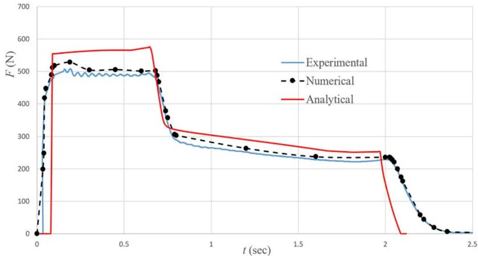
The numerical simulation values are in a marginal similarity to measured values with a relative error of less than $5\mathrm{\%}$ whereas the analytical calculation can predict the thrust with an accuracy of about $15\mathrm{\%}$ relative to the experimental measurements. The deviation between the numerical simulation and the experimental measurements in the transient phases is less than the deviation in the boost and sustain phase, this is due to the relative error occurring during burnback calculation analysis in the boost and sustain phase, but in the transient phases, the grain burn back process doesn't exist. It can be concluded from this comparison that numerical simulations are capable of calculating thrust using measured pressure as an alternative to thrust measurements.

VI. CONCLUSION

An experiment-based numerical simulation and analysis for a dual thrust solid-propellant motor was carried out to investigate the flow features and parameters along the motor and nozzle for the whole working time. This gives more understanding and better insight that cannot be accomplished with experimental measurements. The pressure-time curve from experimental measurements was analyzed to obtain the inputs required for the simulations whereas gas parameters were calculated from thermochemical calculations. The pressure-time curve was divided into two types of simulation, steady-state and transient, the steady-state phase was represented in two phases, boost phase and sustain phase steady-state simulations. The transient phases were represented in three phases, ignition phase, transition (from boost to sustain) phase, and tail off phase. The results from numerical simulation were used to calculate the motor thrust via using the parameters marched out from the motor exit. The thrust values calculated from numerical simulations were compared with the experimental measurements and the error was less than $5\mathrm{\%}$ in all cases. Numerical simulations were confirmed capable of explaining the flow parameters variations with time as well as calculating the motor thrust with a remarkable level of accuracy compared with analytical calculations that are more suited for preliminary calculations.