## I. INTRODUCTION However, like fatig The Gaussian distribution is also commonly known as the Gaussian distribution, and it is generally known that the height, weight, and even IQ of a group of people are relatively consistent with the Gaussian distribution. However, like fatigue life of structures is often far from the Gaussian distribution and more in line with the Weibull distribution. In [1] it was pointed out that the Weibull distribution is a full state distribution, i.e., it can depict not only left-skewed and right-skewed data, but to some extent also symmetric as well as data satisfying a power law. In this sense it is more versatile than the Gaussian distribution [2], [3] and plays a very important role especially in fitting the fatigue life of structures. However, because of the difficulties encountered in determining the three parameters of the Weibull distribution, the problem was solved by taking the logarithm to make the data appear to be more in line with the Gaussian distribution. In fact, this approach is problematic. This paper points out that logging the original data is only a spatial transformation from a mathematical point of view, but from a physical point of view, it changes the structure of the data, and the physical meaning is changed, so it is not appropriate to use logarithmic Gaussian distribution to fit the original data after logarithm. To determine the three parameters of the Weibull distribution, the graphical and analytical methods[4] were previously adopted, the former being inconvenient to use and with relatively large errors; the latter involves solving a system of three joint transcendental equations, which, despite the availability of computers to do so, still has the problem of being inconsistent. This problem can now be solved relatively well by using T.Z. Gao method proposed by [1]. ## II. THE CHARACTERISTICS OF THE GAUSSIAN DISTRIBUTION It is well known[4] that the so-called Gaussian distribution is a distribution in which the random variable is a PDF of $X$ with the form, $$ f(x)=\left[1/(2\pi)^{1/2}\sigma\right]\exp\left[-(x-\mu)^{2}/2\sigma^{2}\right] $$ where $\mu$ and $\sigma^2$ are the mean and variance of the Gaussian distribution, respectively. And when the mean $\mu = 0$ and the standard deviation $\sigma = 1$ is called the standard Gaussian distribution as follows, $$ [1/(2\pi)^{1/2}]\exp(-x^{2}/2) $$ From the definition of Gaussian distribution it is easy to see that Gaussian distribution has the following characteristics[5]: 1. Single-peaked, a distribution that is unimodal. And symmetry, with its Mode and median and mean are the same. 2. Universality, a significant proportion of random variables encountered in real life are or approximately conform to the Gaussian distribution. Even in an arbitrary distribution, in the case of a large sample, the distribution of the mean will approximate the Gaussian distribution. 3. Simplicity, i.e., only two parameters $(\mu, \sigma^2)$ are needed to determine the shape of the entire distribution. Because the normal distribution has so many good characteristics, it has become the most studied and applied distribution. However, it is obvious that not all data conform to Gaussian distribution, and in most cases the data conform to Gaussian distribution is only a good approximation. In fact[4], the data of various fatigue lives are often not fit Gaussian distribution but better fit Weibull distribution, and sometimes the fatigue life is logarithmically distributed, but it is only an approximation. Because of this, Weibull distribution needs to be introduced and studied in more depth. ## III. BRIEF INTRODUCTION OF WEIBULL DISTRIBUTION There are various expressions for the Weibull distribution, and a more general form is taken here[1], with a probability density function: $$ f (x) = (b / \lambda) \left[ \left(x - x _ {0}\right) / \lambda \right] ^ {b - 1} \exp \{- \left[ \left(x - x _ {0}\right) / \lambda \right] ^ {b} \} \tag {3} $$ where $b$ is the shape parameter, $\lambda$ is the scale or proportional parameter, and $x_0$ is called the position parameter. In the field of fatigue it is customary to use the fatigue life $N$ instead of $x$, $N_0$ instead of $x_0$, and call it the safe life. In a non-strict sense[1], "when $0 < b < 1$ resembles a power-law function, while $1 < b < 3$ is a left-skewed distribution, $3 < b < 4$ approximates a Gaussian distribution, and $b > 4$ is a right-skewed distribution". This is the reason why the Weibull distribution is called the "full state distribution". As shown in the following fig.1[5]: 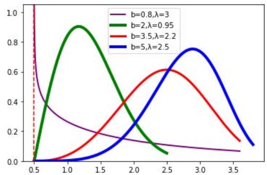 Fig. 1: PDF of various Three-Parameter Weibull distributions when $x_0 = 0.5$ It is easy to prove that the life is $x_{i}$ and the corresponding reliability[1] is, $$ p_{i}=\exp\left\{-\left[\left(x_{i}-x_{0}\right)/\lambda\right]^{b}\right\} $$ It can be seen that when $x = x_0$, $p_0 = 100\%$. This is the origin of $100\%$ reliability safety life. If $p_{50} = 50\%$, it means that the corresponding $X$ is called the median value $x_m$ of $X$, that is, there are, $$ 50\% = \exp \left\{ - \left[ (x_m - x_0) / \lambda \right]^b \right\} $$ It is not difficult to get the expectation and variance of Weibull distribution with three parameters according to the definition[4], $$ \mathrm {E} (X) = x _ {0} + \lambda \Gamma (1 + 1 / b) \tag {6} $$ $$ \operatorname{Var}(X) = \lambda^{2} \left[ \Gamma(1 + 2 / b) - \Gamma^{2}(1 + 1 / b) \right] \tag{7} $$ In this way, the fatigue life data are given and the three parameters of Weibull distribution can be derived by (5), (6) and (7), which is the analytical method. In addition to the analytical method, the maximum likelihood method and some methods derived from it have been used more recently, but they have problems such as cumbersome derivation and inconvenient calculation, so we will not discuss them in depth here. ## IV. ORIGIN OF Z.T. GAO METHOD AND FITTING STANDARD Theoretically if a set of fatigue life data $N$ is given, then using the median $(N_{m})$, mean $(N_{av})$ and mean squared deviation (s) of this array, then using the three equations (5), (6) and (7) is possible to solve for the estimated values of the three parameters of the Weibull distribution. However, for convenience (5), (6) and (7) can be reduced to a transcendental equation[1] with respect to $b$: $$ \left(N _ {a v} - N _ {m}\right) \left[ \Gamma (1 + 2 / b) - \Gamma^ {2} (1 + 1 / b) \right] + s \left[ D ^ {1 / b} - \Gamma (1 + 1 / b) \right] ^ {1 / 2} = 0 \tag {8} $$ where $D = \ln 2$. This equation is solvable by Newton's method, and after obtaining $b$, then $\lambda$ and $N_0$ can be found by (7),(6). Example 1: The data in Table 8-2 in [4] are used to find the three parameters of the Weibull distribution by analytical method. Table 1: A set of fatigue life data (103c) <table><tr><td>124</td><td>134</td><td>135</td><td>138</td><td>140</td></tr><tr><td>147</td><td>154</td><td>160</td><td>166</td><td>181</td></tr><tr><td colspan="5">\(N_{av}=148, N_m=144, s=17.3 \)</td></tr></table> You can get it through Python code, Parameter estimation: $b = 1.221$, $N_0 = 127$, $\lambda = 22.46$ It is not difficult to find that $\mathsf{N}_0(= 127)$ derived from the analytical method is greater than the minimum value of 124 for this group of fatigue lives. And this is in contradiction with the definition of safe life $\mathsf{N}_0$. That is, the problem of inconsistent occurs. Another question is what happens if we fit this set of data with a Gaussian distribution? That is, which is the more appropriate distribution to fit? The second problem can be judged by the magnitude of the determination coefficient[8] $R^2$ fitting the ideal reliability based on the so-called "average rank"[4]. The so-called ideal reliability means that the following formula is independent of the specific distribution, $$ p_{i}=1-i/(n+1) $$ where $i$ is the order of the data from smallest to largest, and $n$ is the number of data. And the first problem is solved by the Z. T. Gao method[1]. The basic idea of the method is briefly described below. Taking the logarithm of both sides of (4) twice yields that $$ \ln \left(\ln \left(1 / p _ {\mathrm{i}}\right)\right) = b \ln \left(\mathrm{N} _ {\mathrm{i}} - \mathrm{N} _ {0}\right) - b \ln (\lambda) \tag{10} $$ $$ if set,\[Y_{i}=\ln(\ln(1/p_{i})),X_{i}=\ln(N_{i}-N_{0})\] $$ $$ d=-b\ln(\lambda),\\lambda=\exp(-d/b) $$ So (10) could be born, $$ Y_{i}=bX_{i}+d\tag{13} $$ This is a system of linear regression equations that can be derived by the least squares method with coefficients $b$ and $d$. However, it is important to note that here $X_{i}$ is related not only to the data $N$ already given, but also to the required safety lifetime $N_{0}$ of Weibull distribution. This problem can be solved by determining the extreme value of the absolute value of the relative coefficient $r$ of the regression line to determine the corresponding $N_{0}$, but the mathematical derivation of this method is complex and error-prone [9]. It is better to use a different idea to use Python to find the series of $r$ about $N_{0}$ directly in the interval $0 \leq N_{0} < N_{\min}$ (here $N_{\min}$ is taken as the minimum value of the given data). Then Python intelligently finds the $N_{0}$ of $r$ with the largest correlation coefficient, and at the same time determines $b$ and $\lambda$. This is known as the Z.T. Gao algorithm. It is abbreviated as the Z.T. Gao method [1], [5] or GZT method. Example 2: Now, using the data of Example 1, three parameters of Weibull distribution are determined by using GZT method, and the results are compared with Gaussian distribution. The results are as follows: 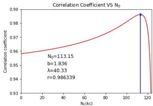 Fig. 2: Schematic graph of Z.T. Gao method This figure graphically demonstrates how GZT method finds the corresponding safe lifetime that maximizes the correlation coefficient. Since it is clear at the beginning of the process that $N_{0}$ cannot be greater than the minimum lifetime of the data, it is not possible to have a situation where it is inconsistent. Again, if the data are fitted with a Gaussian distribution and the coefficient of determination of the Weibull distribution estimated by GZT method, respectively, fitted with the ideal reliability (9): Coefficient of determination obtained by fitting the Weibull distribution $= 0.97999$ Coefficient of determination obtained by fitting the Gaussian distribution $= 0.95044$ It can be seen that the fitted coefficient of determination of the Weibull distribution obtained by GZT method is greater than that of the Gaussian distribution. That is, in this sense the data are more realistically depicted by the Weibull distribution. The advantage of GZT method is that the physical meaning is very intuitive, and there is no problem of "inconsistent". This method is not only convenient for solving the problem of estimating the three parameters of the Weibull distribution, but also easy to determine whether the original data fits better with the Weibull distribution or with the Gaussian distribution. It is also easy to extend to solve similar problems, such as fitting fatigue performance curves with three parameters[1], and the confidence intervals of these three parameters will be discussed in separate papers[10], [11]. ## V. PROBLEMS OF LOGARITHMIZATION OF ORIGINAL DATA Due to the complexity of the Weibull distribution, when the original data is not so consistent with the Gaussian distribution, often take its logarithmic, from a mathematical point of view is equivalent to do a spatial transformation, at this time because the data "compressed", it may be closer to the Gaussian distribution[4]. This has the advantage of making the PDF of the original data taken logarithmically will be fitted quite well by the Gaussian distribution, which will be more convenient for people to study and apply. However, this will lose the physical meaning of the safety lifetime, while making the original data density distribution is "distorted". This is illustrated in the following two examples. Example 3: Using the (large sample) 100 fatigue life data of a structure from Table 12-3 of [1] P253, the Python code gives: Table 2: Gaussian distribution parameters (large sample) <table> <tr> <td></td> <td>Mean</td> <td>s</td> <td>Median</td> <td>r</td> <td>R2</td> </tr> <tr> <td>Original</td> <td>5.315</td> <td>1.289</td> <td>5.07</td> <td>0.99051</td> <td>0.97911</td> </tr> <tr> <td>Take Log10</td> <td>5.713</td> <td>0.101</td> <td>5.705</td> <td>0.99702</td> <td>0.99385</td> </tr> <tr> <td>Recover 10^{\text{log}10}</td> <td>5.164</td> <td>1.262</td> <td>5.07</td> <td>0.99515</td> <td>0.98805</td> </tr> </table> <table> <tr> <td></td> <td>Mean</td> <td>s</td> <td>Median</td> <td>r</td> <td>R2</td> </tr> <tr> <td>Original</td> <td>5.315</td> <td>1.289</td> <td>5.07</td> <td>0.99051</td> <td>0.97911</td> </tr> <tr> <td>Take Log10</td> <td>5.713</td> <td>0.101</td> <td>5.705</td> <td>0.99702</td> <td>0.99385</td> </tr> <tr> <td>Recover 10^\text{log}10</td> <td>5.164</td> <td>1.262</td> <td>5.07</td> <td>0.99515</td> <td>0.98805</td> </tr> </table> Table 3: Weibull distribution parameters (large sample) <table> <tr> <td></td> <td>b</td> <td>N0</td> <td>λ</td> <td>r</td> <td>R2</td> </tr> <tr> <td>Original</td> <td>2.147</td> <td>2.78</td> <td>2.8</td> <td>0.99515</td> <td>0.98903</td> </tr> <tr> <td>Take Loq10</td> <td>3.346</td> <td>5.408</td> <td>0.34</td> <td>0.9961</td> <td>0.99121</td> </tr> </table> <table> <tr> <td></td> <td>b</td> <td>N0</td> <td>\lambda</td> <td>r</td> <td>R^2</td> </tr> <tr> <td>Original</td> <td>2.147</td> <td>2.78</td> <td>2.8</td> <td>0.99515</td> <td>0.98903</td> </tr> <tr> <td>Take Loq10</td> <td>3.346</td> <td>5.408</td> <td>0.34</td> <td>0.9961</td> <td>0.99121</td> </tr> </table>  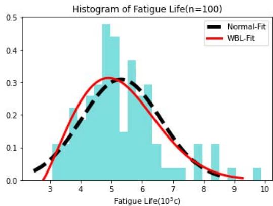Fig. 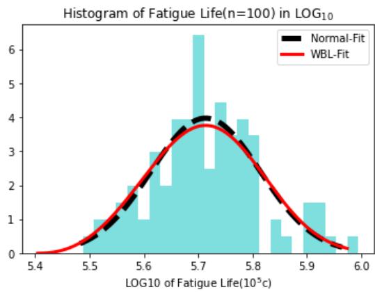3: Histogram of original data (large sample) and fitting diagram of Gaussian and Weibull distribution  Fig. 4: Histogram after logarithm of the original data (large sample) and fitting diagram of Gaussian and Weibull distribution As seen in Fig. 3, the histogram of the original data is asymmetric and left-skewed, and fitting it with a Gaussian distribution would be less appropriate, as in fact demonstrated with the chi-square test[4]. At this point it would be more appropriate to use the Weibull distribution. Looking at the logarithm of the data, we can see from Fig. 4 that the data do appear to be symmetric, and the Gaussian distribution is indeed a good fit. The problem is that the fatigue life PDF left-skewed features are lost, and the physical meaning of safe life is lost. Even if the results obtained in the logarithmic case "back" to the original state, only the median can "recover" (see Table 2, line 3), and the mean is left-skewed, the relative coefficient and the coefficient of determination is improved. Nevertheless, it is still not possible to obtain a $100\%$ safe lifetime. In contrast, the fit with the Weibull distribution, as seen in Table 3, is a fairly good fit. Even after taking the logarithm, the fit is almost the same as that of the Gaussian distribution. From the data in row 2 of the Weibull distribution parameters in Table 3 and (6) and (7), we can calculate that $\mu^{\wedge} = 5.7137$; $\sigma^{\wedge} = 0.1005$ And this result is almost the same as the data in row 2 of Table 2. In this sense the Weibull distribution is indeed more general than the Gaussian distribution, which can be seen as a first-order approximation to the Weibull distribution. It can be seen that using the Weibull distribution to fit this set of fatigue life data does not require any logarithm of the data at all and the physical meaning of each parameter is very clear. Example 4: Looking again at the case of a small sample, 20 data for the life of a structure using Table 8-4 of P136 in [2]. Again, this can be obtained by Python code as follows Fatigue life (raw data) $N =$ [3.5, 3.8, 4.0, 4.3, 4.5, 4.7, 4.8, 5.0, 5.2, 5.4, 5.5, 5.7, 6.0, 6.1, 6.3, 6.5, 6.7, 7.3, 7.7, 8.4](10^5cycle) Also the following parameter table and histogram can be obtained. Table 4: Gaussian distribution parameters (small sample) <table><tr><td></td><td>Mean</td><td>s</td><td>Median</td><td>r</td><td>R2</td></tr><tr><td>Original</td><td>5.57</td><td>1.322</td><td>5.45</td><td>0.99675</td><td>0.98948</td></tr><tr><td>Take Log10</td><td>5.734</td><td>0.103</td><td>5.736</td><td>0.99892</td><td>0.99257</td></tr><tr><td>Recover 10log10</td><td>5.42</td><td>1.268</td><td>5.45</td><td>0.99648</td><td>0.99094</td></tr></table> Table 5: Weibull distribution parameters (small sample) <table><tr><td></td><td>b</td><td>N0</td><td>λ</td><td>r</td><td>R2</td></tr><tr><td>Original</td><td>2.04</td><td>2.766</td><td>3.21</td><td>0.99914</td><td>0.99824</td></tr><tr><td>Take Loq10</td><td>3.588</td><td>5.36</td><td>0.41</td><td>0.99921</td><td>0.9984</td></tr></table>  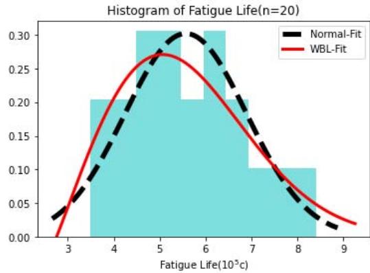Fig. 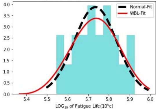5: Histogram of original data (small sample) and fitting diagram of Gaussian and Weibull distribution  Histogram of Fatigue Life(n=20) in $\mathsf{LOG}_{10}$ Fig. 6: Histogram after logarithm of the original data (small sample) and fitting diagram of Gaussian and Weibull distribution As seen in Fig. 5 and 6, similar to the case of the large sample, the original data are also left-skewed and appear symmetric after taking the logarithm. However, if the Weibull distribution is fitted, there is no need to take the logarithm of the original data. Even if the logarithm is taken, the data looks more symmetric, but the Weibull distribution does not fit worse than the Gaussian distribution. So in this sense, even for symmetric data, fitting with the Weibull distribution is possible. However, the difficulty in fitting the Weibull distribution is that it is more difficult to estimate the three parameters, but now there is no problem with GZT method. ## VI. CONCLUSION 1. The three-parameter Weibull distribution is a more general full state distribution than the Gaussian distribution. In the field of reliability, the physical meaning of its position parameter is particularly important, that is, the safe life under $100\%$ reliability. 2. Based on the complexity of the three-parameter Weibull distribution, the previous methods to determine its three parameters by test data are complicated. The graphical method is more error-prone and inconvenient to use; while the analytical method may be inconsistent; and the GZT method makes full use of the advantages of Python, which solves this problem better. 3. In the past, the fatigue life data that were not so well fitted with Gaussian distribution were taken logarithmically so that they might be more consistent with Gaussian distribution, but the result of doing so made the $100\%$ reliability of the safe life no longer exist. The fact is that the data itself is more consistent with Weibull distribution. Since Weibull distribution is a full state distribution, it is generally not necessary to take the fatigue life as logarithm in the future and directly fit the fatigue life data with the three-parameter Weibull distribution to get a better fit. 4. The two parameters of Gaussian distribution (mean and variance) are not very significant for asymmetric data, while for asymmetric data like structural fatigue life the three parameters of Weibull distribution (safety life, shape and scale parameters) will be much more significant, and in a sense these three parameters "contain" the two parameters of Gaussian distribution. This is probably the reason why the Weibull distribution can "contain" the Gaussian distribution. 5. Finally, it can be concluded that for asymmetric fatigue life, it is not necessary to take logarithms to fit with Gaussian distribution, but can be directly fitted with three-parameter Weibull distribution. Further even for the more symmetric data, it is better to fit directly with the three-parameter Weibull distribution. ### ACKNOWLEDGMENTS We thank Mr. Wan Weihao for his support to this paper and related research work.

Generating HTML Viewer...

References

9 Cites in Article
J Xu (2021). Gao Zhentong Method in the Fatigue Statistics Intelligence.
Waloddi Weibull (1951). A Statistical Distribution Function of Wide Applicability.
Arthur Hallinan (1993). A Review of the Weibull Distribution.
No ethics committee approval was required for this article type.
Data Availability
Not applicable for this article.
How to Cite This Article
Xu Jiajin. 2026. \u201cFrom Gaussian Distribution to Weibull Distribution\u201d. Global Journal of Research in Engineering - I: Numerical Methods GJRE-I Volume 23 (GJRE Volume 23 Issue I1): .
Explore published articles in an immersive Augmented Reality environment. Our platform converts research papers into interactive 3D books, allowing readers to view and interact with content using AR and VR compatible devices.
Your published article is automatically converted into a realistic 3D book. Flip through pages and read research papers in a more engaging and interactive format.
The Gaussian distribution is one of the most widely used statistical distributions, but there are a lot of data that do not conform to Gaussian distribution. For example, structural fatigue life is mostly in accordance with the Weibull distribution rather than the Gaussian distribution, and the Weibull distribution is in a sense a more general full state distribution than the Gaussian distribution. However, the biggest obstacle affecting the application of the Weibull distribution is the complexity of the Weibull distribution, especially the estimation of its three parameters is relatively difficult. In order to avoid this difficulty, people used to solve this problem by taking the logarithm to make the data appear to be more consistent with the Gaussian distribution. But in fact, this approach is problematic, because from the physical point of view, the structure of the data has changed and the physical meaning has changed, so it is not appropriate to use logarithmic Gaussian distribution to fit the original data after logarithm. The author thinks that Z.T. Gao method can give the estimation of three parameters of Weibull distribution conveniently, which lays a solid mathematical foundation for Weibull distribution to directly fit the original data.
Our website is actively being updated, and changes may occur frequently. Please clear your browser cache if needed. For feedback or error reporting, please email [email protected]
Thank you for connecting with us. We will respond to you shortly.