I. INTRODUCTION

For the last half century, the early years of each decade saw a major turning point in the world economy and markets. Each country began with a global mania for some big idea, some new change agent that reshaped the world economy and generated huge profits. It was the boom of the major economies around the world. The 2010s brought in the era of emerging markets: Brazil, Russia, India, China and South Africa. These poor economies were growing rapidly as well as erratically from 4 percent to 12 percent a year. However, this was so far the fastest growth spurt to be ever experienced across the world (Sharma, 2012). Thus, the question of political regimes came forward, as each of these five newly emerging economies has a different political system. The newly emerging economies portrayed a different political system – from authoritarian China to socialist Russia to democratic South Africa, Brazil to a multi-party parliamentary system in India. Thus, it becomes imperative to assess the impact of political system and its stability on economic growth. The political system of a nation is described in its Constitution. Constitutions establish the governance structures of nation states, provinces, and supranational organizations such as the

European Union. In designing constitutions, arguably the most important issue is to determine the extent to which collective decision-making should be centralized (Bodenstein and Ursprung, 2001).

Political stability plays a very important role in achieving economic growth. Many studies have been undertaken to determine the impact of political stability on economic growth. Most of the studies have attempted to establish this relationship by taking countries from a particular region or countries having similar pattern of governance (Alesina et al, 1992; Feng, 1997; Barro, 1994; Bildirici, 2004; Salvi, 2005; Jhee, 2006; Hazama, 2009; Aisen and Veiga, 2011; Acemoglu and Robinson, 2012; Nomor and Iorember, 2017).

In a country like India, the federal structure of political system ensures that the Constitution is well guarded and abided by the rule-makers. With the multitude of parties that exists in India, coalition government becomes necessary.

In the economic literature the interest in the relationship between political instability and economic performance is very well established. This leads to inefficient public expenditure, deficit and debt accumulation, distorted investment and ultimately lower economic growth. However, the large amount of contributions in the political science literature on coalition politics suggest that a few other mechanisms could be active and that the definition of political instability should also account for the interaction between the executive and the legislature (Carmignani, 2001).

The question that we try to answer here is – whether the economic growth that takes place in India is affected by stability at the central and states level political situation.

II. THEORETICAL UNDERPINNING

This section provides the theoretical justification for the analysis of political stability and economic growth in India with its federal structure in background.

In India, Salvi (2005) attempted to establish a relationship between political stability and economic growth with Lok Sabha election results (Lower House of the Parliament). However, Rajya Sabha (Upper House of the Parliament) results have been left out of the scope. India has a federal structure and both the Houses play an important role in passing of a Bill, which ultimately becomes a Law. Hence, in order to estimate the political stability, the strength of the ruling party/ruling alliance needs to be gauged in both the Houses.

Furthermore, no study has been attempted to establish the relationship of political stability and economic growth for the states in India. Many theoretical studies have attempted to define political stability at the state level; but none of them have attempted to measure the impact of political stability and economic growth/development. (Salvi, 2005; Nooruddin and Chhibber, 2008).

Let us understand first, the structure of Indian Federalism, the formation of Indian states and the existing multi-party system of Indian polity.

a) Indian Polity: Federal Structure

After independence, India adopted the parliamentary form of democracy with a federal character. The Constituent Assembly or the Parliament in India is bi-camera in nature. The Lower House is the House of the People, called as Lok Sabha; and the Upper House is the Council of States, called as Rajya Sabha (Nag, 2013).

Lok Sabha is representative of people in India. The members are elected representatives by simple majority in general elections. The maximum number of elected membership for Lok Sabha is 552 elected members and 2 Anglo-Indian members nominated by the President, if not already returned through election. Seats are allotted to each state in proportion to its population. Presently, there are 543 members of the Lok Sabha. The tenure of Lok Sabha is of five years (Nag, 2013).

The List of Lok Sabha seats from each of the states is given in Table 1.

No.	Name of States/Union Territories	No. of Constituencies
1	Andhra Pradesh	25
2	Arunachal Pradesh	2
3	Assam	14
4	Bihar	40
5	Chhattisgarh	11
6	Goa	2
7	NCT of Delhi	7
8	Gujarat	26
9	Haryana	10
10	Himachal Pradesh	4
11	Jammu and Kashmir	6
12	Jharkhand	14
13	Karnataka	28
14	Kerala	20
15	Madhya Pradesh	29
16	Maharashtra	48
17	Manipur	2
18	Meghalaya	2
19	Mizoram	1
20	Nagaland	1
21	Odisha	21
22	Punjab	13
23	Puducherry	1
24	Rajasthan	25
25	Sikkim	1
26	Tamil Nadu	38
27	Telangana	17
28	Tripura	2
29	Uttar Pradesh	80
30	Uttarakhand	5
31	West Bengal	42
32	Andaman and Nicobar Islands	1
33	Chandigarh	1
34	Dadra and Nagar Haveli	1
35	Daman and Diu	1
36	Lakshadweep	1
	Total	542

Rajya Sabha members are elected by the elected members of the State Legislative Assemblies. It is not subject to dissolution as Rajya Sabha is the permanent body. However, one third of its members retire every two years and are replaced by newly elected members. Yet, each member is elected for a term of six years. The maximum strength of Rajya Sabha is 250 members. Currently, the strength is 245 members; out of which 233 are elected from States and Union territories and 12 are nominated by the President from distinguished fields. The number of members is in proportion to the population of the States (Nag, 2013).

The state wise List of Rajya Sabha seats is given in Table 2.

No.	State/Union Territories	No of Seats	No of Members	Vacancies
1	Andhra Pradesh	11	11
2	Arunachal Pradesh	1	1
3	Assam	7	7
4	Bihar	16	15	1
5	Chhattisgarh	5	5
6	Goa	1	1
7	Gujarat	11	11
8	Haryana	5	5
9	Himachal Pradesh	3	3
10	Jammu & Kashmir	4	4
11	Jharkhand	6	6
12	Karnataka	12	12
13	Kerala	9	9
14	Madhya Pradesh	11	11
15	Maharashtra	19	19
16	Manipur	1	1
17	Meghalaya	1	1
18	Mizoram	1	1
19	Nagaland	1	1
20	National Capital Territory of Delhi	3	3
21	Nominated	12	12
22	Odisha	10	9	1
23	Puducherry	1	1
24	Punjab	7	7
25	Rajasthan	10	9	1
26	Sikkim	1	1
27	Tamil Nadu	18	17	1
28	Telangana	7	7
29	Tripura	1	1
30	Uttar Pradesh	31	30	1
31	Uttarakhand	3	3
32	West Bengal	16	16
	Total:	245	240	5

b) Working of the Parliament

Legislative proposals can be introduced in either Houses of the Parliament in the form of a Bill. When passed by both the Houses and assented by the President, the Bill becomes a Law, an Act of the Parliament. Money Bills can be introduced only in the Lok Sabha; the Rajya Sabha can only make recommendations over the Bills, within a period of fourteen days (Nag, 2013).

Thus, in measuring political stability, both the Houses of the Parliament are taken into consideration. The ruling party's strength in both the houses needs to be measured as it affects the policy-decisions through legislative procedures.

At the state level, the corresponding bodies are Vidhan Sabha (Legislative Assembly or the Lower House) and Vidhan Parishad (Legislative Council or the Upper House). All the states in India have a Vidhan Sabha. However, only a few major states with a high population have bi-camera state legislature. These states are Andhra Pradesh, Bihar, Jammu and Kashmir, Karnataka, Maharashtra, Telangana and Uttar Pradesh (Nag, 2013).

The list of Vidhan Sabha seats according to states is given in Table 3

No.	States	Vidhan Sabha		Vidhan Parishad
		1952	2019	1952	2019
1	Andhra Pradesh	-	175	-	58
2	Arunachal Pradesh	30 ('78)	60	-	-
3	Assam	105	126	-	-
4	Bihar	330	243	72	75
5	Chhattisgarh	-	90	-	11
6	Goa	30 ('67)	40	-	-
7	Gujarat	154 ('62)	182	-	-
8	Haryana	81 ('67)	90	-	-
9	Himachal Pradesh	36	68	-	-
10	Jammu & Kashmir	75 ('62)	87	-	36
11	Jharkhand	-	81	-	14
12	Karnataka	99	224	63	75
13	Kerala	126 ('67)	140	-	-
14	Madhya Pradesh	232	230	-	-
15	Maharashtra	315	288	40	78
16	Manipur	30 ('67)	-	-	2
17	Meghalaya	60 ('72)	60	-	-
18	Mizoram	30 ('72)	40	-	-
19	Nagaland	40 ('64)	60	-	-
20	Orissa	140	147	-	-
21	Punjab	126	117	-	-
22	Rajasthan	160	200	-	-
23	Sikkim	32 ('79)	32	-	-
24	Tamil Nadu	375	234	-	-
25	Telangana	-	119	-	40
26	Tripura	30 ('67)	60	-	-
27	Uttar Pradesh	430	403	72	100
28	Uttarakhand	-	70	-	-
29	West Bengal	238	294	-	-
	Union Territories
30	Andaman & Nicobar	-	NA	-	-
31	Chandigarh	-	NA	-	-
32	Dandra& Nagar Haveli	-	NA	-	-
33	Daman & Diu	-	NA	-	-
34	Delhi	48	70	-	-
35	Lakshadweep	-	NA	-	-
36	Pondicherry	30 ('64)	30	-	-

c) Reorganisation of the states

India is a country of a wide variety of ethnic groups and minorities. By the time India attained freedom in 1947, it was partitioned. This was not anticipated by the then Congress leaders who had a prominent role in nation-building. They had to join a territorially disjoint country characterised by huge diversity, into a single union of a nation state. It is under this backdrop that India chose to adopt a federal structure and the Constitution was drafted accordingly (Sarangi, 2013). Ultimately, the Constitution was framed in such a way that most of the powers for law-making decisions were kept with the central state. Thus, the leaders gave a federal, parliamentary, and democratic constitution on 26th January.

1950. The Constitution divided governmental powers and responsibilities into three distinct lists:

1. The first - exclusively under the jurisdiction of the central state called as Union List;

2. The second- largely under the jurisdiction of the state units called as State List; and

3. The third - to be shared by the central and the states governments called as Concurrent List.

This distribution was meant to accommodate differences in strong central government (Chadda, 2002).

After the consolidation of the Indian Union in 1950, there had been three major waves of reorganisation of the states. First major reorganisation occurred in 1956, following a nationwide movement for the creation of linguistically compact provinces by Tamils, Sikhs and the Muslim Community (Kashmir). The second major initiative came in the 1970s, when the Northeast was split up and several new states were created. The third phase was inaugurated with the creation of Jharkhand, Uttaranchal and Chhattisgarh in the northern Hindi-Hindu belt provinces (Chadda, 2002). At present, there are 28 States and seven Union Territories. The dates of the formation of States and the Union Territories is shown in the table.

The list of dates of formation of the States and Union Territories is given in Table 4.

No.	States/Union Territories	Date of Formation
1.	Andhra Pradesh	1 November 1956
2.	Arunachal Pradesh	20 February 1987
3.	Assam	15 August 1947
4.	Bihar	1 April 1936
5.	Chhattisgarh	1 November 2000
6.	Goa	30 May 1987
7.	Gujarat	1 May 1960
8.	Haryana	1 November 1966
9.	Himachal Pradesh	25 January 1971
10.	Jammu & Kashmir	26 October 1947
11.	Jharkhand	15 November 2000
12.	Karnataka	1 November 1956
13.	Kerala	1 November 1956
14.	Madhya Pradesh	1 November 1956
15.	Maharashtra	1 May 1960
16.	Manipur	21 January 1972
17.	Meghalaya	21 January 1972
18.	Mizoram	20 February 1987
19.	Nagaland	1 December 1963
20.	Odisha	1 April 1936
21.	Punjab	1 November 1956
22.	Rajasthan	1 November 1956
23.	Sikkim	16 May 1975
24.	Tamil Nadu	26 January 1950
25.	Telangana	2 June 2014
26.	Tripura	21 January 1971
27.	Uttar Pradesh	26 January 1950
28.	Uttarakhand	9 November 2000
29.	West Bengal	1 November 1956
	UNION TERRITORIES
1.	Andaman & Nicobar	1 November 1956
2.	Chandigarh	1 November 1966
3.	Dadra & Nagar Haveli	11 August 1961
4.	Daman & Diu	23 May 1987
5.	Delhi	1 November 1992 (NCT)
6.	Lakshadweep	1 November 1956
7.	Puducherry	1 July 1963

d) General Lok Sabha Elections

The federal structure of the Indian state took a backseat in the initial years immediately after independence. The Indian National Congress (INC) party was India's party of government in the first five successive parliamentary elections: 1951, 1957, 1962,

1967 and 1971. It was like a one-party dominant system (Booroah, 2006). The Congress government under Nehru was the need of the hour for an India that had been totally messed up by British misrule (Rai and Kumar, 2017).

The general election in 1971 was contested by Indira Gandhi on the slogan "GaribiHatao" and her pro-poor posturing created an electoral wave in her favour. The elections sorted out the leadership issue once and for all with Indira Gandhi acquiring a larger than life image equated with the Indian goddess Durga and starting a new chapter that became known as the personality cult in Indian politics (Rai and Kumar, 2017). The second tier leadership in the party and voice for constructive criticisms was destroyed as she replaced state leaders with people who had no political base and were completely loyal to her. The electorates had no way of communicating with the Congress leadership like it previously could. Due to this, the Congress party lost many bye-elections subsequently. There was high inflation due to Pakistan war and 1973 oil crisis, led to decline in faith of people on the Congress party. Her falling popularity and Allahabad High Court ruling on electoral malpractices led to the declaration of emergency in 1975. She circumvented the parliament and ruled the country by imposing her dictatorship by sacrificing parliament and democratic rights of the people (Rai and Kumar, 2017).

The Congress Party was overthrown in general elections, 1977 by unification of opposition parties as the Janata Party. Just before 1977 elections, four national parties, viz. Indian National Congress (O), Bhartiya Lok Dal, Bhartiya Jan Sangh and the Socialist Party, merged formally to form Janata Party (Salvi, 2005). The Janata Party came to power from 1977-1979. By July, 1979, Janata Party split into two - one led by Chandrashekhar (JP) and other led by Charan Singh (JP(S)). JP(S) soon became Lok Dal (Chander, 2004, Salvi, 2005).

After a brief period out of power, following the 1977 elections; the Congress stormed back winning the next two elections (1980 and 1984) handsomely (Chander, 2004; Booroah, 2006). After the assassination of Indira Gandhi, Congress party won 1984 elections under the leadership of Rajiv Gandhi with 415 seats mainly due to the sympathy wave. The party lost its political presence and single party dominance in the 1989 General elections due to Bofors scam. The BJP won a considerable number of seats in 1989 elections only to form a coalition with the Janata Dal (JD) led National Front (Chander, 2004; Salvi, 2005; Rai and Kumar, 2017).

The decade of 1990s was a turmoil in Indian politics due to frequent elections and weak coalitions at the Centre as regional parties came, gained importance and raised to power.

In 1991, Congress came back to power and remained the largest political party till 1996. However, the BJP attained the status of the second-largest party in the 1991 elections. In the 1996 elections, the Congress, emerged as the single-largest party but short of majority. Therefore, it chose to sit on the opposition benches. The minority government which was a coalition of 13 parties came to power under the leadership of H. D. DeveGowda. The Congress gave outside support to this government. Congress pulled out its support due to Rajiv Gandhi assassination issue. Thus in 1996, the Congress party was the supporter of the minority government being on the opposition bench (Chander, 2004).

Mid-term elections were called for in the 1998, when BJP led coalition government was formed under the leadership of A. B. Vajpayee. However, AIADMK chief Jayalalitha pulled out due to a minor issue for a minister and the Vajpayee government lost confidence motion by just one vote (Chander, 2004).

Once again, elections were called in 1999. The BJP emerged as a dominant party, however, was way short of majority. The coalition government was formed with 24 parties forming an alliance. This government survived its five year term (Chander, 2004).

Congress was again able to form a government after the 2004 elections in coalition with other parties and supported, by the communists, from outside government.

The UPA II government was inundated by numerous scams, high inflation and unemployment rates and the policy paralysis that hit the country in the last two years of its regime by middle of 2009 (Chander, 2004; Salvi, 2005; Sridharan, 2005; Booroah, 2006).

The Congress was wiped out in the general election in 2014. The BJP came to power with comfortable majority. The BJP received support from regional parties like Shiv Sena, Telugu Desam Party, Shiromani Akali Dal, and other smaller parties. The alliance of these parties is called as National Democratic Alliance (NDA); whereas, in the opposition, there were Congress, BahujanSamajwadi Party, Communist Party of India, Nationalist Congress Party, All India Trinamool Congress and many other smaller parties (Rai and Kumar, 2017).

The coalition era has created a pattern of tide. Relative centralization of power at first, followed by a steady erosion of power as the results of the state elections (held almost every two years) alters the composition of parliamentary majority for the ruling coalition (Chadda, 2002).

e) State Assembly Elections

The regional parties in India play a very important role in the state as well as central politics. This is due to three major reasons. First, it was the decline of the Congress party as the dominant party in terms of its traditional social support base, organizational presence, and ideology that paved the way for state parties to emerge. Second, in seven consecutive Lok Sabha elections (1989-2009) no single party could win a majority of seats, resulting in "minority situations"; and hence, minority governments were dependent on external support. Third, the Bharatiya Janata Party (BJP) has been instrumental in making alliances with state parties even agreeing to become a junior ally. Though these alliances have helped the BJP, they have also helped state parties confront the weakened Congress and allowed their bosses to gain in stature at the national level. A national/regional/multi-state party confines itself to a coded ethnic card in selection of candidates, but not openly in its identification of issues. As a result, state-level parties have greater power to create and retain a core social constituency, which in turn, becomes a distinct voting community. This is the politics of vote bank which gets them elected. A large number of state parties are set up by leaders from the same caste and communities. They launch their "own" parties which dominate state politics and influence as a coalition ally at the state level with no significant role at the Centre (Chandra, 2005).

Important links have been identified between political leadership and economic development. In post-1991 India, state-level leaders such as Chandrababu Naidu, Chimanbhai Patel, and S.M. Krishna took advantage of the new economic climate to think of novel ways to encourage growth in the states under their command, instead of looking towards the Centre for policy directions and all their funds as in the old "socialist" days. It was in the 1990s that states under such dynamic leadership grew much faster than others; whereas, Bihar under Lalu Yadav registered a zero growth rate in the same decade. The Congress has suffered many defeats in Andhra Pradesh and Telangana after losing Y.S. Rajsekhara Reddy (YSR) and Jaganmohan Reddy, who formed the YSR Congress party after being denied a leadership role by the Congress. Even in a cadre-based party like the BJP, which takes pride in being a disciplined party, powerful state-level leaders (like Narendra Modi and Vasundhara Raje Scindia, to name a few) have taken up posts of high importance within the party high command (Rai and Kumar, 2017).

Captain Amarinder Singh, the present chief minister of Punjab, had threatened to start his own party. The success of the BJP in the 2014 elections had much to do with the popularity of its state leaders (in Chhattisgarh, Madhya Pradesh, and Rajasthan). The Congress high command consciously encouraged factionalism within the party's state units to weaken its state leaders and hence, lost. It would be far-fetched to overemphasize the ability of state-level leaders, however, especially from polity-wide parties such as the

BJP and Congress to shape out independent political spaces.

The Karnataka Janata Paksha, the party set up by the BJP leader and former chief minister (erstwhile rebel) Yeddyurappa, performed poorly, winning only six assembly seats and polling about 10 percent of the votes in the 2012 assembly elections. The Gujarat Parivartan Party, founded by the former chief minister Keshubhai Patel, another disgruntled powerful state-level BJP leader belonging to the dominant Patel community, failed miserably in electoral terms in the 2012 assembly elections with just two seats and 4 percent of the vote share. The Himachal Lokhit party, founded by BJP rebel Maheshwar Singh in Himachal Pradesh, was another failure. Thus, there is always a question mark on the extent to which state-level leaders belonging to a polity-wide party, howsoever popular and powerful they may be when in power, can influence/mobilize voters without the umbrella of the big party. (Rai and Kumar, 2017).

There are other non-Congress political leaders such as E.M.S.Namboodiripad or even Jyoti Basu, both essentially state-level leaders with a national presence due to their influence over the Communist party. Chaudhary Charan Singh thrived in becoming famous at national level after becoming Prime Minister.

As the boundaries between state-level parties and the state units of national parties have become hazy, one found state leader such as Mamata Banerjee is trying to affect national-level policy decisions. Despite nurturing national ambitions, however, what remains a handicap for state-level leaders such as Mulayam Singh Yadav, Mayawati, Mamata Banerjee, or Nitish Kumar is their lack of nation-wide stature, given their perceived susceptibility to falling prey to regional and parochial interests to the detriment of national cause (Chander, 2004).

The Dravidian parties have been very vocal about their regionalism. The AIADMK and the DMK in Tamil Nadu have allocated seats to ensure majorities for themselves. This has prevented the emergence of coalition governments in the state so far. The AIADMK and the DMK can also represent themselves as natural parties of government, as they alone have been able to rule the state with a democratic mandate since 1967. This is particularly important where voters esteem the prospect of winning when deciding how to cast their vote. The ideological discipline of the parties has, for a number of reasons, been brought into question. The willingness of both parties to ally with the BJP does not reflect well on their rationalist background. (Chander, 2004).

f) Research design

i. Variables and Data

With this political backdrop, an attempt is made here to measure political stability in India and in its states. Political stability is measured by constructing an index by using the following variables.

a. General Elections and Raya Sabha Elections: (India level)

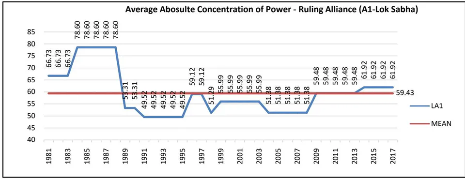
Absolute Concentration of Power in Lok Sabha: Concentration of power is the number of seats that a party wins from the total seats in the House. It is also the proportion of seats that the major party or the alliance enjoys in the House (Salvi, 2005; Younis et al, 2008; Bernal-Verdugo et al, 2013). Absolute Concentration of Power is the number of seats that a party/alliance - ruling or opposite - wins in proportion to the total number of seats in the House. Absolute Concentration of Power is measured with respect to ruling party/alliance as well as opposition party/alliance. Absolute Concentration of Power (A1) is given as below:

Absolute Concentration of Power

India enjoyed single party government till 1989 election where the Congress was the only and major ruling party at the Centre. After 1989 election, the era of coalition governments dawned upon Indian politics. Thus, the number of seats that major ruling party (MRP) along-with the coalition parties that it has partnered with (Ruling Alliance) in proportion to the total number of seats in the House is called as Absolute Concentration of Power (ACP). The Absolute Concentration of Power of the Ruling Party/Alliance variable (A1) is essential to measure political stability as it judges the ability/strength of the Ruling Party to pass a law in the Parliament. On the other hand, the Absolute Concentration of Power of the Opposition party/alliance variable (A2) helps to judge the strength of the opposition/hurdle that the government faces in passing of the Bill.

Thus, for Ruling Party/Alliance, Absolute Concentration of Power (A1) is given as:

ACP (A1)

For Opposition Party/Alliance, Absolute

Concentration of Power (A2) is given as:

ACP (A2)

For example, in 1984 Lok Sabha General Election, the Congress party won absolute majority in the House. It won 404 seats out of 514 seats. There was no alliance formed. Hence, Congress was the major ruling party. The Ruling Alliance's Absolute Concentration of Power (A1) is given as 66.37 percent. $(404/{514}^{\ast }100={0.6637}^{\ast }100=66.37$ percent) This shows that the government at the Centre is strong enough and stability can be sustained. Higher the value of A1, better is the political stability. Therefore, A1 has a positive relationship with political stability as government formed will be stronger.

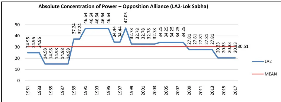
In 1984 election, the major opposition party (BJP) won only 22 seats. Whereas, the opposition coalition parties won 55 seats. Hence, a coalition of opposition parties was formed $(22+55=77$ seats). The Opposition Alliance's Absolute Concentration of Power (A2) is given as 14.98 percent (77/514100 =0.1498100=14.98 percent). This shows that opposition is weak enough to stall/halt the daily working and decision-making of the Parliament. This ensures more political stability. Lower the value of A2, better is the political stability. Therefore, A2 has a positive relationship with political stability as opposition will be weaker, not affecting the longevity or continuity of policies and also, of the government formed.

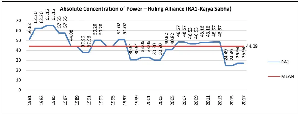
Absolute Concentration of Power in Rajya Sabha: Similarly, for 1984 Rajya Sabha election, the ruling party (Congress) had 159 seats out of total of 244 seats. Hence, the Ruling Alliance's Absolute Concentration of Power (A1) is given as 65.16 percent $(159/{244}^{\ast }100={0.6516}^{\ast }100=65.16$ percent).

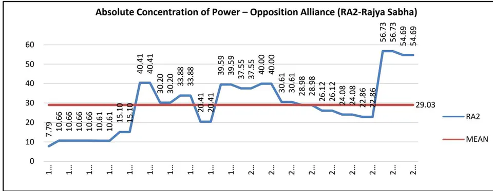
The major opposition party (BJP) won only 12 seats. Whereas, the opposition coalition parties won 14 seats. Hence, a coalition of opposition parties was formed (12+14=26 seats). The Opposition Alliance's Absolute Concentration of Power (A2) is given as 10.66 percent (26/244100=0.1066100=10.66 percent).

Relative Concentration of Power in Lok Sabha: In order to form the government, a simple majority or a coalition majority is required in the House. This is measured by the Absolute Concentration of Power variable. However, for effective and smooth functioning of the government, Relative Concentration of Power (RCP) is essential. Relative Concentration of Power is the number of seats that the major ruling party wins in proportion to the total number of seats of the alliance it has formed in the House (Salvi, 2005; Younis et al, 2008; Bernal-Verdugo et al, 2013). A non-protected policymaker (party not having majority in the House, or having small majority) may have very little interest in trying to "push through" reform if he knows that ex-post, he can easily be blocked. On the other hand, a much protected leader may have stronger motivations to reform and legislative activity (Aghion et al, 2002).

For the Major Ruling Party, Relative Concentration1of Power (R1) measures its strength within the coalition that it enters to form the government.

Major Ruling Party's Relative Concentration of Power within the Total Ruling Coalition (R1) is given as:

The Major Ruling Party's Relative Concentration of Power variable (R1) is essential to measure political stability of the major ruling party as it judges the ability/strength of the Ruling Party to form the cabinet, pass a law in the Parliament and also, to control internal disputes and bickering within the alliance.

Also, in order to assess the Total Ruling Alliance's strength, comparatively to total opposition seats; the Relative Concentration of Power is measured with respect to Total Opposition Alliance (Salvi, 2005).

Thus, Ruling Alliance's Relative Concentration of Power with respect to Opposition Alliance is given as:

On the other hand, the Ruling party/Alliance's Relative Concentration of Power variable (R2) helps to judge the strength of the Ruling alliance in the overall working of the House.

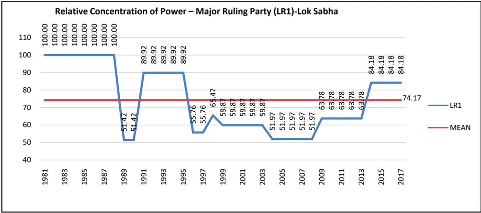
For example, in 1984 Lok Sabha General Election, the Congress party won absolute majority in the House. It won 404 seats out of 514 seats. There was no alliance formed. Hence, Congress was the only ruling party. The Major Ruling Party's Relative Concentration of Power (R1) is given as 100 percent $(404/{404}^{\ast }100=1^{\ast }100=100$ percent). In this case, the Major Ruling Party is at its strongest. Higher the value of R1, better is the political stability as the major ruling party will have better decision-making powers.

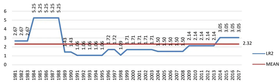
In 1984 election, the major opposition party (BJP) won only 22 seats. Whereas, the coalition parties won 55 seats. Hence, a coalition of opposition parties was formed. $(22+55=77$ seats) The Ruling Alliance's Relative Concentration of Power (R2) is given as 5.25 times $(404/77=5.25$ times). This shows that the Ruling Alliance is 5.25 times stronger than the Opposition Alliance in terms of seats won.

Relative Concentration of Power – Ruling Alliance vs. Opposition Alliance (LR2)-Lok Sabha Figure 8: India mean chart of R2-LokSabha

Relative Concentration of Power in Rajya Sabha: Similarly, for Rajya Sabha, the ruling party had 159 seats out of total of 244 seats and there was no alliance.

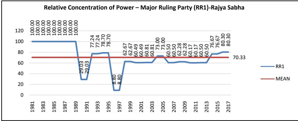
Hence, the Major Ruling Party's Relative Concentration of Power (R1) is given as 100 percent $(159/{159}^{\ast }100=1^{\ast }100=100$ percent).

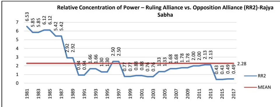
The major opposition party (BJP) won only 12 seats. Whereas, the opposition coalition parties won 14 seats. Hence, a coalition of opposition parties was formed $(12+14=26$ seats). The Ruling Alliance's Relative Concentration of Power (R2)) is given as 6.12 times (159/26=6.12 times). The Ruling Alliance is 6.12 times stronger than total opposition alliance in terms of seats won. Higher the value of R2, better is the political stability as government formed will be stronger.

b. State Elections

On the same basis, for the state elections, the seats won by the ruling part/ alliance or opposition party/alliance are taken in proportion to the total seats of the Vidhan Sabha (State Legislative Assembly) for absolute concentration of power (ACP).

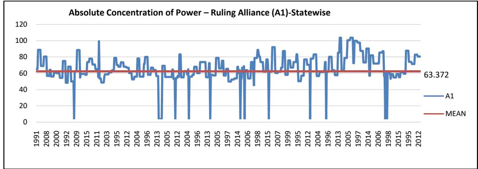
For example, for 1987 West Bengal state election which corresponds to the year 1990, the total seats of the Vidhan Sabha were 294. The Major Ruling Party won 187 seats and its alliance partners won 64 seats. Thus, total Ruling Alliance won 251 seats $(187+64=251)$. Hence, the Ruling Alliance's Absolute Concentration of Power (A1) is given as 85.37 percent $(251/294\ast 100=0.8537\ast 100=85.37$ percent).

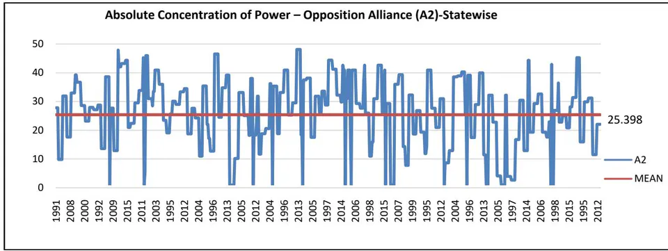
Whereas the Major Opposition Party won 40 seats and its alliance partners won 3 seats. Thus, the Opposition Alliance won 43 seats $(40+3=43)$. Hence, the Opposition Alliance's Absolute Concentration of Power (A2) is given as 14.63 percent $(43/{294}^{\ast }100={0.1463}^{\ast }100=14.63$ percent).

On the same basis, for the state elections, the seats won at the Vidhan Sabha (State Legislative Assembly) by the ruling party/alliance or opposition party/alliance are taken in consideration.

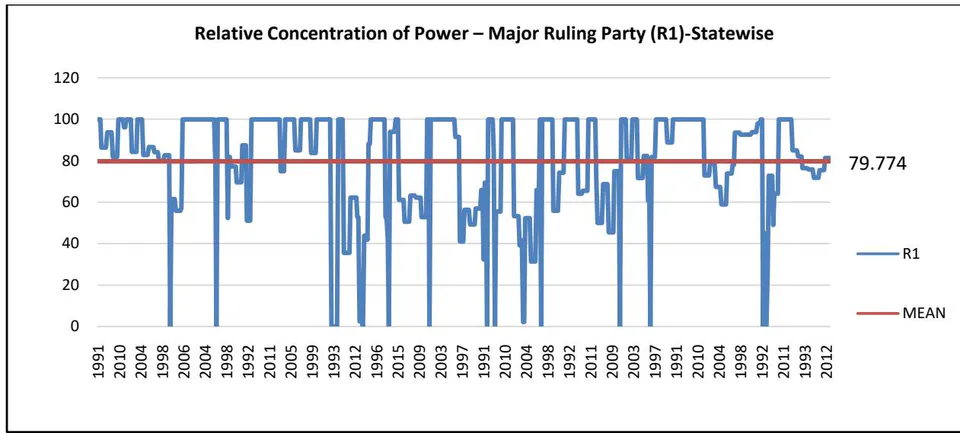
For example, for 1987 West Bengal state election, corresponding to the year 1990, the total seats of the Vidhan Sabha were 294. The Major Ruling Party won 187 seats and its alliance partners won 64 seats. Hence, total Ruling Alliance won 251 seats $(187+64=251)$. Hence, the Major Ruling Party's Relative Concentration of Power (R1) is given as 74.50 percent $(187/251\ast 100=0.745\ast 100=74.50$ percent).

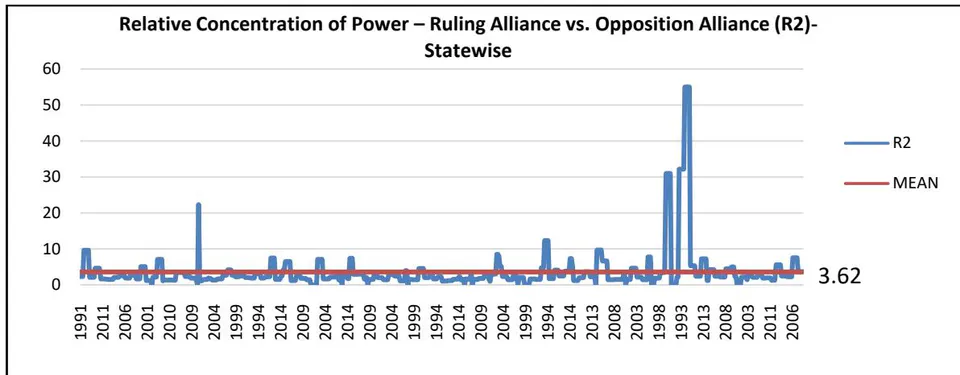
Whereas the Major Opposition Party won 40 seats and its alliance partners won 3 seats. Hence, the Opposition Alliance won 43 seats $(40+3=43)$. Hence, the Ruling Alliance's Relative Concentration of Power (R2) is given as 5.84 times $(251/43=5.84$ times).

The electoral data has been collected from statistical reports of all the General Lok Sabha elections (national level) as well as Vidhan Sabha elections (States level) since 1981 onwards; available on the Election Commission of India website (http://eci.nic.in/eci main1/ElectionStatistics.aspx).

For Rajya Sabha, data has been collected from 'Rajya Sabha Statistical Information 1952-2013' and also from the Election Commission of India website (http://eci.nic.in/eci main1/ElectionStatistics.aspx).

The information on the alliances of the Ruling and Opposition parties over all the General elections till 2004 election as well as states of West Bengal and Kerala elections till 2004, has been collected from Chander (2004). Various news reports of prominent magazines, newspapers and media channels were referred for Lok Sabha 2009 and 2014 Alliances and as well as state elections. (Detailed List provided at the end).

We construct an index of political stability using all the dependent variables at the India level as follows:

• Political stability Index (PLSI):

• India Level Political Stability Index (PLSI_IND)

First, we construct four indicators to measure political stability at all India using election data of the lower house of the Parliament i.e. Lok Sabha. Another four indicators are constructed using data from the upper house of the Parliament i.e. Rajya Sabha. Thus, we have eight variables at India level. They are:

1. Absolute Concentration of Power – Ruling Alliance (LA1)

2. Absolute Concentration of Power - Opposition Alliance (LA2)

3. Relative Concentration of Power - Major Ruling Party (LR1)

4. Relative Concentration of Power - Ruling Alliance vs. Opposition Alliance (LR2)

5. Absolute Concentration of Power – Ruling Alliance (RA1)

6. Absolute Concentration of Power - Opposition Alliance (RA2)

7. Relative Concentration of Power - Major Ruling Party (RR1)

8. Relative Concentration of Power - Ruling Alliance vs. Opposition Alliance (RR2)

In order to find which prominent indicators of political stability have a significant impact on the economic growth of the nation, Principal Component Analysis is carried out (Filmer and Pritchett, 2001; Hatcher et al, 2013).

Technically, Principal component analysis is a variable reduction procedure, defined as a linear combination of optimally-weighted observed variables. These variables, thus obtained, may then be used as predictor or criterion variables in following analyses. (Filmer and Pritchett, 2001; Hatcher et al, 2013). It is useful when there is some redundancy in those variables. In this case, redundancy means that some of the variables are correlated with one another, possibly because they are measuring the same constructor when data is obtained on a number of variables (possibly a large number of variables). Due to this redundancy, the observed variables can be possible to reduce into a smaller number of principal components (artificial variables) that will comprise most of the variance in the observed variables (Filmer and Pritchett, 2001; Hatcher et al, 2013). The number of components extracted in a principal component analysis is equal to the number of observed variables being analysed (Filmer and Pritchett, 2001; Hatcher et al, 2013). This means that an analysis of n-variables would actually result in n components. However, in most analyses, only the first few components account for meaningful amounts of variance (usually, with values higher than one). Hence, only these first few components are retained, interpreted, and used in subsequent analyses (such as in multiple regression analysis) (Filmer and Pritchett, 2001; Hatcher et al, 2013).

The first principal component has the maximum value of loading. This loading is squared and is used as weight to construct the political stability index. The Principal Component analysis is carried out in order to reduce the matrix and find the most effective indicators which explain almost $80\mathrm{\%}$ of the variance. Then, the relevant artificial variables are defined on the basis of eigenvalues which account for most of the variance. Usually, it is first three to four variables that define up to approximately $80-85\mathrm{\%}$ of the variance. In our analysis, first three values are defined as pc1, pc2 and pc3 (Principal Components). (Usually the components with eigenvalues greater than one are selected to define the new components.) (Filmer and Pritchett, 2001; Hatcher et al, 2013)

The loadings (eigenvectors multiplied by square root of eigenvalues) are extracted. The loadings are the covariances between the original variables and the unit scaled components. The eigenvalues are magnitude/variances of the variables while the eigenvectors are the direction of the variables. The value of squared loadings of each of the variables serve as weight for construction of the political stability index. The square of loadings portrays the contribution of a principal component into that variable. (Filmer and Pritchett, 2001; Hatcher et al, 2013)

Since, the first principal component (pc1) usually defines most of the variance; the loading of each of the variables under pc1 is squared. These respective squared loadings serve as weights for that respective variable. Thus, each variable is multiplied by the respective squared loading under pc1. The sum of the weighted variables, thus derived, form the political stability index.

Thus, higher value of political stability index means better stability and lower value means political stability is weak, i.e. considerable extent of political instability exists in the system. (Filmer and Pritchett, 2001; Hatcher et al, 2013).

For example, for India in 1981, the variables value (and loadings; squared loadings after the Principal Component Analysis) are as under:

1. LA1 = 66.73 (0.413; 0.170569)
2. LA2 = 24.95 ((-0.337); 0.113569)
3. LR1 = 100 (0.318; 0.101124)
4. LR2 = 2.67 (0.395; 0.156025)
5. RA1 = 50.82 (0.312; 0.097344)
6. RA2 = 7.79 ((-0.318); 0.101124)
7. RR1 = 100 (0.308; 0.094864)
8. $\mathsf{RR}\mathsf{2}=6.53$ (0.406; 0.164836)

The new values are derived after multiplying the variables' original value with the values of squared loadings as shown below:

1. $|A|=11.38$ (66.730.170569) 2. $|A2|=2.83$ (24.950.113569) 3. $\left|R1\right|=10.11(100\ast 0.101124)$ 4. $\left|R2\right|=0.42\left(2.67\ast 0.156025\right)$ 5. rA1l = 4.95 (50.820.097344) 6. rA2l = 0.79 (7.790.101124) 7. $rR11=9.48(100\ast 0.094864)$ 8. $rR2I=1.08({6.53}^{\ast }0.164836)$

These weighted values are added to construct the political stability index as under:

For the remaining years of time series (1981-2017), the PLSIND index is constructed with similar method.

Summary Statistics, using the observations 1981 - 2017
Variable	Mean	Median	Minimum	Maximum
LA1	59.429	59.116	49.520	78.599
LA2	30.511	32.781	14.981	47.048
LR1	74.169	63.777	51.418	100.00
LR2	2.3208	1.7166	1.0617	5.2468
RA1	44.093	46.531	24.490	65.164
RA2	29.029	28.980	7.7869	56.735
RR1	70.334	73.000	8.8000	100.00
RR2	2.2821	1.6761	0.43165	6.5263
Variable	Std. Dev.	C.V.	Skewness	Ex. kurtosis
LA1	9.1858	0.15457	1.0094	0.051564
LA2	9.9179	0.32506	0.086387	-0.76971
LR1	18.852	0.25418	0.20953	-1.6071
LR2	1.3170	0.56751	1.3470	0.67197
RA1	11.427	0.25915	-0.019749	-0.76814
RA2	13.878	0.47808	0.33108	-0.59494
RR1	23.950	0.34052	-0.77697	0.61077
RR2	1.8958	0.83075	1.1940	0.00062371
Variable	5% Perc.	95% Perc.	IQ range	Missing obs.
LA1	49.520	78.599	10.541	0
LA2	14.981	46.682	11.796	0
LR1	51.418	100.00	32.107	0
LR2	1.0617	5.2468	1.3598	0
RA1	24.490	65.164	17.451	0
RA2	10.330	56.735	21.837	0
RR1	8.8000	100.00	29.647	0
RR2	0.43165	6.1565	1.8290	0

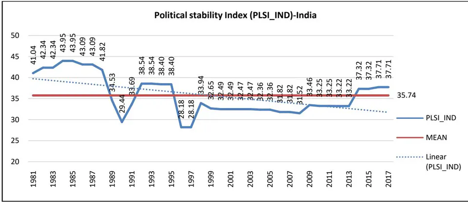
Then, independent 'Regression Analysis' is carried out to determine the effect of the political stability index on each of the economic growth indicators at the

India level; The model articulates that the independent variables may have a significant impact on the dependent variable.

OLS Regression is carried out at India level to assess the impact of PLSI on economic growth indicators.

Secondly, the analysis carried out at India level within the same time period as General election results are taken into consideration.

The analysis is carried out using 'Gretl' software.

State Level Political Stability Index (PLSI_STE)

At the state level, only six major states have an upper house of the Legislative Assembly. Hence, the state level upper house is kept out of the purview of the scope of the study. Thus, we have four variables measuring political stability at the state level (due to consideration of only Vidhan Sabha) and independent Panel Regression is carried out to find the dependence of each of the economic growth indicators on political stability index at the States level.

At the States level, the indicators constructed are:

1. Absolute Concentration of Power – Ruling Alliance (A1)
2. Absolute Concentration of Power - Opposition Alliance (A2)
3. Relative Concentration of Power - Major Ruling Party (R1)
4. Relative Concentration of Power - Ruling Alliance vs. Opposition Alliance (R2)

Correspondingly, at states level, the Political Stability Index (PLSI_STE) is developed in the similar way using the four indicators that we have constructed.

For example, for Andhra Pradesh in 1991, the variables values (and loadings; squared loadings after the Principal Component Analysis) are as under:

1. $A1=61.56$ (0.6; 0.36)
2. $\mathsf{A}2=26.87$ ((-0.463); 0.214369)
3. $R1=100$ (0.3; 0.09)
4. $R2=2.29$ (0.579; 0.335241)

The new values are derived after multiplying the variables' original value with the values of squared loadings as shown below:

1. A1l = 22.16327 (61.56*0.36)
2. A21 = 5.76025 (26.87*0.214369)
3. $R1I=9$ (100*0.09)
4. R2l = 0.768084 (2.29*0.335241)

These weighted values are added to construct the political stability index as under:

For the remaining years of time series (1991-2015) and rest of the states' cross-sections (28), the PLSI_STE is constructed with similar method.

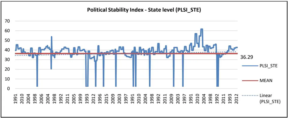
Variable	Mean	Median	Minimum	Maximum
A1	62.372	60.147	0.00000	100.00
A2	25.398	27.143	0.00000	47.143
R1	79.774	86.400	0.00000	100.00
R2	3.6268	2.1579	0.00000	55.000
Variable	Std. Dev.	C.V.	Skewness	Ex. kurtosis
A1	16.219	0.26004	-1.0373	4.3142
A2	11.619	0.45750	-0.44454	-0.44715
R1	24.441	0.30638	-1.4189	1.8915
R2	6.1484	1.6953	6.0094	41.404
Variable	5% Perc.	95% Perc.	IQ range	Missing obs.
A1	46.181	86.752	18.034	0
A2	0.94017	42.222	15.739	0
R1	35.556	100.00	34.409	0
R2	0.55000	8.2250	1.9169	0

However, at the States level, a lag of one year is taken into consideration due to the fact that different states have Assembly elections in different years. Hence, the term of State Assemblies is also different. Hence, considering this discrepancy in the frequency of the Assembly elections, we have taken a lag period of one year.

Since, the time series (1991-2015) as well as cross-sections (28 states) remain fixed, fixed-effect model is estimated. As Judson and Owen (1996), discussed that for most macroeconomic dataset, fixed-effect model is more appropriate as the dataset is fixed in terms of the time-period as well as cross-sections.

To study the impact of political stability on economic growth, first an attempt is made to estimate variables through which economic growth is measured. These variables are as follows:

c. Dependent (Economic Growth) Variables

> India Level

Growth rate of the real Per Capita Income (PCI_GR): The real GDP per capita income is considered as a broad and the most basic indicator of economic development of a nation. The real per capita GDP is calculated from the nominal Gross State Domestic Product data. The nominal GDP and GSDP data on Indian states was collected from the RBI's 'Handbook of Statistics of Indian States (2017-18)' and also Niti Aayog website (http://niti.gov.in/state-statistics#.). Also, the reports available on the Planning Commission of India website were accessed (http://planningcommission.nic.in/data/ datatype/). Lastly, the various State Economic Survey reports were accessed for the missing data/figures.

The GSDP data at current prices (with base 2011=100) was, then, calculated from the available GSDP data at various price levels using splicing method. The population data for India and every state level was collected from the Census data (https://www.census2011.co.in/states.php).

Since, census is conducted every 10 years in India, the population numbers for inter-census years is not available. Hence, the method of interpolation was used to estimate the population for inter-census years.

For example, for ten year period between 1991 and 2001 census, the population figures for 1991 and 2001 are available. The two figures are added and divided by two to get the figure for 1995. Then 1991 and 1995 figures are added and divided by two to get the figure for 1993 and so on and so forth. The per capita income was calculated from the GDP/GSDP data from the population figures, thus, interpolated.

The growth rate of real per capita income was calculated on the basis of the below mentioned equation:

where,

PCI GR - the growth rate of real per capita income; PCI - the real per capita income in the period t.

${\mathsf{PCI}}_{l-1}$ - the real per capita income in the period t-1.

Gross Capital Formation as a percentage of GDP (GCFGDP): The Gross Capital Formation is the total value of the gross fixed capital formation (outlays on fixed assets), changes in inventories and acquisitions less disposals of valuables for all the sectors of the economy. Fixed assets include land improvements; plant, machinery, and equipment purchases; and the construction of infrastructure. Inventories are amount of goods held by firms to meet temporary or unexpected variations in production. The valuables are defined as investments in precious metals, stones, artefacts, and so on which do not contribute to further production in the economy. However, their value appreciates/ depreciates on the basis of economic and market conditions. When people save, they tend to invest. The percentage of the investments in fixed capital inventories, acquisitions and valuables made each year out of the total GDP is called Gross Capital Formation as percentage of GDP (World Bank National Accounts data (World development indicators, 2018); Samuelson and Nordhaus, 2012).

Thus, Rate of Gross Capital Formation (GCF as percentage of GDP) is defined as follows:

The importance of the GCF lies in the fact that it is that part of GDP that is invested which, in turn, helps in the growth of the GDP itself. This is essential in achieving high growth of production, capital formation, changes in production techniques and launching the economy on the growth path (Samuelson and Nordhaus, 2012).

The India level GCF as percentage of GDP data is available from the World Bank database from 1981-2017 (https://data.worldbank.org/indicator/NE.GDI.TOT L.ZS?locations=IN).

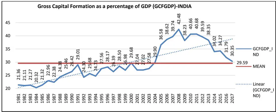
The following table gives the descriptive statistics of both the economic growth variables.

Summary Statistics, using the observations 1981 - 2017
Variable	Mean	Median	Minimum	Maximum
PCI_GR	4.4454	4.2694	-0.16280	9.2144
GCFGDP	29.590	27.583	20.319	42.476
Variable	Std. Dev.	C.V.	Skewness	Ex. kurtosis
PCI_GR	2.4704	0.55572	0.13458	-0.90793
GCFGDP	6.5947	0.22286	0.49599	-0.97850
Variable	5% Perc.	95% Perc.	IQ range	Missing obs.
PCI_GR	0.41676	8.9717	3.9815	0
GCFGDP	21.033	40.861	10.870	0

The growth rate of per capita income (PCI_GR_IND) as independent variable and gross capital formation as a percentage of GDP (GCFGDP_IND) as another independent variable. The analysis is individually carried out for both the economic indicators. The correlation between both the independent variables at India level is 0.5. Hence, it can be considered as moderate level correlation and independent analysis can be carried out.

Correlation coefficients, using the observations 1981 - 2017

5% critical value (two-tailed) = 0.3246 for n = 37, with two-tailed p-value 0.0016

	PCI_GR_IND	GCFGDP_IND
PCI_GR_IND	1.0000	0.5013
GCFGDP_IND		1.0000

First, the per capita growth rate is taken as independent variable and regression analysis is carried out. The results are obtained. Then, the gross capital formation as a percentage of GDP is taken as independent variable and regression analysis is carried out to obtain the results.

States Level

Growth rate of the real Per Capita Income (PCI_GR_STE): The state level growth rate of the real per capita income is calculated in the same way as at the India level. For example, for Andhra Pradesh at current prices (2011=100), the real ${\mathsf{PCI}}_{1990}=\mathsf{Rs}.3888.468$ and ${\mathsf{PCI}}_{1991}=\mathsf{Rs}.4632.032$. Hence the PCI GR will be $19.12\mathrm{\%}$ [(4632.032-3888.468)/3888.468]*100 = [(743.564)/38 88.468]100 = 0.1912100 = 19.12%]

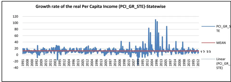
Gross Capital Formation as a percentage of GDP (GCFGDP): At the state level, data for absolute GCF figures (Rs. Million) are only available. The GCF as percentage of GDP is calculated at the states level using the following formula.

Where GSDP is the Gross State Domestic Product

Furthermore, absolute GCF figures are available only from 1990-2015 in the RBI's 'Handbook of Statistics of Indian States (2017-18)'. Hence, due to unavailability of data, the time period for state level analysis is taken from 1991-2015.

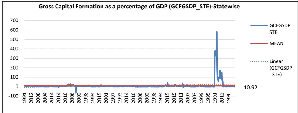
Summary Statistics, using the observations 1:01 - 26:25
Variable	Mean	Median	Minimum	Maximum
PCI_GR	12.330	11.309	-30.981	109.62
GCFGDP	10.921	3.2840	-66.485	580.70
Variable	Std. Dev.	C.V.	Skewness	Ex. kurtosis
PCI_GR	10.236	0.83012	4.1698	32.703
GCFGDP	44.199	4.0471	8.1006	75.553
Variable	5% Perc.	95% Perc.	IQ range	Missing obs.
PCI_GR	1.7753	22.833	7.1822	0
GCFGDP	0.0070448	19.115	5.8635	0

The growth rate of per capita income (PCI_GR_STE) as independent variable and gross capital formation as a percentage of GDP (GCFGDP_STE) as another independent variable. The analysis is individually carried out for both the economic indicators. The correlation between both the independent variables at India level is 0.025. Hence, the correlation is low and independent analysis can be carried out.

Correlation coefficients, using the observations 1:01 - 26:25

5% critical value (two-tailed) = 0.0769 for n = 650, with two-tailed p-value 0.04158

	PCI_GR_STE	GCFGSDP_STE
PCI_GR_STE	1.0000	0.0255
GCFGSDP_STE		1.0000

First, the per capita growth rate is taken as independent variable and regression analysis is carried out. The results are obtained. Then, the gross capital formation as a percentage of GDP is taken as independent variable and regression analysis is carried out to obtain the results.

III. AN ANALYSIS

a) Aim

The aim of this study is to analyse the impact of political stability on economic growth for India as well as for 28 states in India. For the purpose of analysis, time period considered is of 37 years from 1981 to 2017 at India level; and time period of 25 years from 1991 to 2015 at the states level. The time period considered is strictly governed by the availability of data. The data set for India is a simple time series data of 37 years (1981-2017). However, the dataset for the states is a panel data spread across time series of 26 years (1990-2015) and cross sections of 28 states. (Arunachal Pradesh and Mizoram are kept out of purview of the analysis due to data unavailability. Also, union territories of Daman, Diu and Dadra Nagar Haveli, Andaman and Nicobar, Chandigarh and Lakshadweep are also kept out of purview as they have no impact on the election data).

India and state level analysis are kept separate due to federal structure of the polity, though regional parties play a very important role in political scenario of the country.

b) Model Specification

We are trying to find out the impact of political stability on economic growth. Political stability is measured by various indicators as described above. In a multi-party system like India, the number of effective parties, the changes in voter preferences (swing in votes), the number of seats that these parties win at every election in the Lok Sabha and the number of seats they occupy in both the Lok Sabha as well as Rajya Sabha (absolute concentration of power); and the coalitions formed, their relative strength and power (relative concentration of power) play a very important role in determining the stability of a government. The growth rate of real per capita income and the gross capital formation as percentage of GDP serve as appropriate measures of economic growth.

Time Period and Cross-Section specifications:

The formation of Indian states was fully completed by the year 1980. However, complete gross capital formation (GCF) data at the state level is available from 1990 onwards. Hence, for India level analysis, the time period in the analysis undertaken is from 1981-2017; whereas for state level analysis, it is from 1990-2015, to account for growth rate of the real per capita SDP and GCF.

The complete election data from the first year (1981) of the time frame is available for India as well as for 27 states, except 3 states, namely Chhattisgarh, Jharkhand and Uttarakhand. The states of Chhattisgarh,

Jharkhand and Uttarakhand were formed in the year 2000. The first elections took place in the year 2002 for Chhattisgarh, 2005 for Jharkhand and 2003 for Uttarakhand.

Hence, there are some variations in the time period as well as cross-section specifications for a few states as mentioned below:

1. Due to unavailability of GCF data, the state level analysis is carried out for a period of 26 years from 1990 - 2015. However, national level analysis is carried out for a period of 37 years from 1981 - 2017 due to availability of GCF data at national level.

2. The time period undertaken for Chhattisgarh is 2004-2015; for Jharkhand, it is 2005-2015; and for Uttarakhand, it is 2003-2015.

3. The National Capital Region of Delhi (Delhi) and Union Territory of Puducherry are taken into analysis as they have a considerable impact on the national as well as state level political decisions. The GSDP data of Delhi and Puducherry is in official records only onwards the year 1993. Hence, the time period for Delhi and Puducherry is 1994-2015.

4. The states of Arunachal Pradesh and Mizoram have been excluded from the study due to unavailability of GCF data.

5. The Bihar State Assembly election in February 2005 had resulted in the President's Rule and mid-term election was held in October 2005. Hence, for the purpose of calculation, the results of the mid-term election are considered.

6. The state of Telangana was formed in the year 2014. Hence, the analysis couldn't be carried out in light of only one election (2014) that has taken place till 2015.

7. The Union Territories of Andaman and Nicobar Islands, Chandigarh, Dadra Nagar Haveli, Daman and Diu and Lakshadweep are also kept out of purview of the analysis as they have negligible to no impact on the political scenario/decisions in the country.

8. The state of Jammu and Kashmir is considered to be a whole state as during the time period of the study (1990-2015), the state was not split up into union territories.

The time period of years between two consecutive elections is also taken into consideration to, appropriately measure the impact of inter-election per capita income and gross capital formation on the voting pattern of the electorates.

No.	State/Union Territories	Time Frame (Years)	Election Years	Number of Elections
1	Andhra Pradesh	1981-2017 (37)	1978, 1983, 1985, 1989, 1994, 1999, 2004, 2009, 2014	09
2	Arunachal Pradesh**	1981-2017 (37)	1980, 1984, 1990, 1995, 1999, 2004, 2009, 2014	08
3	Assam	1981-2017 (37)	1978, 1983, 1985, 1991, 1996, 2001, 2006, 2011, 2016	09
4	Bihar	1981-2017 (37)	1980, 1985, 1990, 1995, 2000, (Oct)2005, 2010, 2015	08
5	Chhattisgarh	2003-2017 (15)	2003, 2008, 2013	03
6	Delhi	1993-2017 (25)	1993, 1998, 2003, 2008, 2013, 2015	06
7	Goa	1981-2017 (37)	1980, 1984, 1989, 1994, 1999, 2002, 2007, 2012, 2017	09
8	Gujarat	1981-2017 (37)	1980, 1985, 1990, 1995, 1998, 2002, 2007, 2012, 2017	09
9	Haryana	1981-2017 (37)	1977, 1982, 1987, 1991, 1996, 2000, 2005, 2009, 2014	09
10	Himachal Pradesh	1981-2017 (37)	1977, 1982, 1985, 1990, 1993, 1998, 2003, 2007, 2012, 2017	10
11	Jammu & Kashmir	1981-2017 (37)	1977, 1983, 1987, 1996, 2002, 2008, 2014	07
12	Jharkhand	2005-2017 (13)	2005, 2009, 2014	03
13	Karnataka	1981-2017 (37)	1978, 1983, 1985, 1989, 1994, 1999, 2004, 2008, 2013	09
14	Kerala	1981-2017 (37)	1980, 1982, 1987, 1991, 1996, 2001, 2006, 2011, 2016	09
15	Madhya Pradesh	1981-2017 (37)	1980, 1985, 1990, 1993, 1998, 2003, 2008, 2013	08
16	Maharashtra	1981-2017 (37)	1980, 1985, 1990, 1995, 1999, 2004, 2009, 2014	08
17	Manipur	1981-2017 (37)	1980, 1984, 1990, 1995, 2000, 2002, 2007, 2012, 2017	09
18	Meghalaya	1981-2017 (37)	1978, 1983, 1988, 1993, 1998, 2003, 2008, 2013	08
19	Mizoram**	1981-2017 (37)	1979, 1984, 1987, 1989, 1993, 1998, 2003, 2008, 2013	09
20	Nagaland	1981-2017 (37)	1977, 1982, 1987, 1989, 1993, 1998, 2003, 2008, 2013	09
21	Odisha	1981-2017 (37)	1980, 1985, 1990, 1995, 2000, 2004, 2009, 2014	08
22	Puducherry	1993-2017 (25)	1991, 1996, 2001, 2006, 2011, 2016	06
23	Punjab	1981-2017 (37)	1980, 1985, 1992, 1997, 2002, 2007, 2012, 2017	08
24	Rajasthan	1981-2017 (37)	1980, 1985, 1990, 1993, 1998, 2003, 2008, 2013	08
25	Sikkim	1981-2017 (37)	1979, 1985, 1989, 1994, 1999, 2004, 2009, 2014	08
26	Tamil Nadu	1981-2017 (37)	1980, 1984, 1989, 1991, 1996, 2001, 2006, 2011, 2016	09
27	Telangana**	2014-2017*	2014*	01*
28	Tripura	1981-2017 (37)	1977, 1983, 1988, 1993, 1998, 2003, 2008, 2013	08
29	Uttar Pradesh	1981-2017 (37)	1980, 1985, 1989, 1991, 1993, 1996, 2002, 2007, 2012, 2017	10
30	Uttarakhand	2002-2017 (16)	2002, 2007, 2012, 2017	04
31	West Bengal	1981-2017 (37)	1977, 1982, 1987, 1991, 1996, 2001, 2006, 2011, 2016	09

c) Estimation Method/Methodology

Many estimation techniques are available for estimation of a panel data. The effects specification for panel analysis is very important. For macroeconomics dataset, the fixed effects model is a common choice. It is generally more appropriate than a random effects model for many macro datasets for two reasons. First, it is highly likely that these country-specific characteristics are correlated with the other regressors only if the individual effect represents omitted variables. Second, a typical macro panel will contain cross section data and, thus, will be less likely to be a random sample from a much larger universe of dataset. (e.g., an OECD panel is likely to contain all of the OECD countries and not just a random sample of them) (Judson and Owen, 1996).

Similarly, for the study, the Indian states analysis contains a total of 28 states and Union Territories. Also, the time period is fixed for the analysis. Thus, a fixed-effect model is more appropriate to our dataset because the likeliness of observations to be random is also very tiny.

Furthermore, we need to remove redundant variables so that internally correlated variables do not affect the analysis. In order to filter the variables, we adopt the Principal Component Analysis.

Principal component analysis is appropriate when we have obtained measures on a number of observed variables and wish to develop a smaller number of artificial variables (called principal components) that will account for most of the variance in the observed variables. After obtaining the principal components, a weighted index is created – political stability index – and regression analysis is carried out to check for dependence of the variables.

d) Hypothesis

We define the model using null hypothesis and alternate hypothesis. Also, the algebraic equation is mentioned below in order to study the impact of the variables.

Null Hypothesis $(H_0)$

The political stability index does not have a significant effect on the economic growth at both the levels - national (1981-2017) as well as the State Legislative Assembly Elections (for 28 states from 1991-2015).

Alternative Hypothesis $(H_t)$

The political stability index have a significant effect on the economic growth at both the levels - national (1981-2017) as well as the State Legislative Assembly Elections (for 28 states from 1990-2015).

Theoretically, at India level, the model can be defined as follows:

where,

PCI_GR_INDt - Growth Rate of Per Capita Income for the period t

GCFGDP_IND - Gross Capital Formation as a percentage of GDP for the period t

PLSI_IND - index constructed using political stability indicators for the period t at India level

${\beta }_k$ - the coefficients to be estimated

$c_m$ - the intercepts; and

${\mu }_{\mathrm{t}}$ -the error term.

However, at the states level, Panel Regression is carried out to assess the relationship between the political stability index and economic growth indicators, separately. First, the per capita growth rate is taken as independent variable and regression analysis is carried out. The results are obtained. Then, the gross capital formation as a percentage of GSDP is taken as independent variable and regression analysis is carried out to obtain the results. Thus, we have a Model 1 and Model 2 at both –India as well as States level.

However, at the States Level, the model can be defined as follows:

PCI_GR_STEt - Growth Rate of Per Capita Income for the period t

GCFGSDP_STE - Gross Capital Formation as a percentage of GSDP for the period t

PLSI_STEt - index constructed using political stability indicators for the period t at states level

PLSI_STEt-1 - index constructed using political stability indicators for the Lag period

${\beta }_k$ - the coefficients to be estimated

$c_{\mathrm{m}}$ - the intercepts; and ${\mu }_t$ -the error term.

e) Results

Here an attempt is made to analyse whether there exists an impact of political stability on economic growth in India.

f) India level results

The major question addressed here is: whether the economic growth that takes place in India is affected by stability at the central and states level political situation?

Model 1: OLS, using observations 1981-2017 (T = 37) Dependent variable: PCI_GR_IND Model 2: OLS, using observations 1981-2017 (T = 37)

	Coefficient	Std. Error	t-ratio	p-value
Const	9.54652	3.16813	3.013	0.0048	***
PLSI_IND	-0.142727	0.0879435	-1.623	0.1136
Mean dependent var	4.445426		S.D. dependent var	2.470393
Sum squared resid	204.3257		S.E. of regression	2.416170
R-squared	0.069988		Adjusted R-squared	0.043416
F(1, 35)	2.633929		P-value(F)	0.113577
Log-likelihood	-84.11347		Akaike criterion	172.2269
Schwarz criterion	175.4488		Hannan-Quinn	173.3628
Rho	0.143589		Durbin-Watson	1.683188

Dependent variable: GCFGDP_IND

	Coefficient	Std. Error	t-ratio	p-value
Const	59.8225	7.09768	8.428	<0.0001	***
PLSI_IND	-0.845882	0.197024	-4.293	0.0001	***
Mean dependent var	29.59043		S.D. dependent var	6.594668
Sum squared resid	1025.537		S.E. of regression	5.413045
R-squared	0.344967		Adjusted R-squared	0.326252
F(1, 35)	18.43245		P-value(F)	0.000133
Log-likelihood	-113.9587		Akaike criterion	231.9174
Schwarz criterion	235.1393		Hannan-Quinn	233.0533
Rho	0.844288		Durbin-Watson	0.301708

The equations of the model can, now, be stated as follows:

Centre and State-level data was analysed. The results prove that there is an impact on the economic growth. However, at India level, there is no significant impact on growth rate of per capita income (R squared $=0.07$, p=0.1136). Thus, it can be seen that p value is not significant at $1\mathrm{\%}$, $5\mathrm{\%}$ or $10\mathrm{\%}$ level of significance. Thus we say that the per capita income growth rate is not affected by the stability of the government.

However, there exists a significant impact on the gross capital formation of the country (R squared = 0.34, p=0.0001). The p-value is significant at all the levels of significance (1%, 5% and 10%). Thus, we can say that investments are impacted by the stability of the government at the Centre and, through investment, it influences the level of income and standard of living of the people.

In a country like India, with a multi-party system and rampant coalition governments, stability of the government is difficult. The Indian political scenario has been dented with frequent, early mid-term elections; pulling out support from existing functioning governments. This may be due to the nature of Indian politics for one decade. Furthermore, frequent imposition of presidential/governor rule. The negative coefficient, thus, indicates that economic growth is adversely affected by political stability indicators.

The coefficient of the index reflects lower values indicating a considerable amount of instability in the country. The Indian political system is plagued by multi-party system where coalition government has become the norm and hence, low value of political stability index per se.

Economic growth tends to get hampered if concentration of ruling alliance is lower, and/or opposition alliance is higher. There will be hurdles created in smooth functioning of the administrative decision- making and implementation as weaker governments are formed. The average of concentration of the ruling party in the total seats at India level in Lok Sabha is approx. 59 percent and in Rajya Sabha is approx. 44 percent (mean of Ruling Alliance in total seats in Lok Sabha-Absolute Concentration LA1=59.42% and mean of Ruling Alliance seats in total seats in Rajya Sabha- Absolute Concentration RA1=44.09%). Similarly at states level, the mean of Ruling Alliance's Concentration of Power is approx. 62

g) State Level Results

percent (mean of Ruling Alliance seats in total seats Absolute Concentration A1=62.18%). This shows that the government is formed by marginal seats in most of the elections. Thus, the strength of the coalition is weaker. This affects political stability adversely as lesser concentration of seats with ruling alliance leads to dicey government, affecting decision-making power regarding economic policies. There will be constant pushes and pulls of the junior/coalition partners in the government.

Since 1990s, the ruling alliance in India has been winning marginal seats as compared to earlier years. When Congress was the dominant party in the 1960s and 1970s, there have been $100\mathrm{\%}$ majority governments. Over the years, the dominance has been lost, paving way for coalition governments; once comprising up to 24 small and big, regional and central political parties.

The proportion of seats of the major ruling party in the ruling alliance also, has been decreasing over the years. This is one of the main reasons, why the composition of coalition has been becoming wider and complicated. The average of concentration of the major ruling party in the total ruling alliance seats at India level in the Lok Sabha is approx. 74 percent and in Rajya Sabha is approx. 70 percent respectively (mean of Major Ruling Party seats in total Ruling Alliance seats in Lok Sabha-Relative Concentration $\text{LR1}=74.17\mathrm{\%}$ and mean of Major Ruling Party seats in total Ruling Alliance seats in Rajya Sabha- Relative Concentration $\text{RR1}=70.33\mathrm{\%}$ ).

Thus, the coefficient of Political Stability index (PLSI) at both-India and the states-levels portray a negative sign. However, our analysis prove that the indicators have a considerable impact on the economic growth of India.

Model 1: Pooled OLS, using 648 observations Included 26 cross-sectional units Time-series length: minimum $=24$ maximum $=25$ Dependent variable: PCI_GR_STE

	Coefficient	Std. Error	t-ratio	p-value
Const	11.5324	2.17060	5.313	<0.0001	***
PLSI_STE	-0.118405	0.0623607	-1.899	0.0580	*
PLSI_STE_1	0.140024	0.0623662	2.245	0.0251	**
Mean dependent var	12.31617		S.D. dependent var	10.24745
Sum squared resid	67351.34		S.E. of regression	10.21864
R-squared	0.008689		Adjusted R-squared	0.005615
F(2, 645)	2.826680		P-value(F)	0.059943
Log-likelihood	-2424.059		Akaike criterion	4854.119
Schwarz criterion	4867.540		Hannan-Quinn	4859.325
Rho	0.047610		Durbin-Watson	1.900247

Model 2: Pooled OLS, using 648 observations

Included 26 cross-sectional units

Time-series length: minimum = 24, maximum = 25

	Coefficient	Std. Error	t-ratio	p-value
Const	72.6654	9.08479	7.999	<0.0001	***
PLSI_STE	-0.722521	0.261003	-2.768	0.0058	***
PLSI_STE_1	-0.978322	0.261026	-3.748	0.0002	***
Mean dependent var	10.93234		S.D. dependent var	44.26696
Sum squared resid	1179819		S.E. of regression	42.76888
R-squared	0.069424		Adjusted R-squared	0.066539
F(2, 645)	24.05962		P-value(F)	8.36e-11
Log-likelihood	-3351.734		Akaike criterion	6709.468
Schwarz criterion	6722.890		Hannan-Quinn	6714.675
Rho	0.828294		Durbin-Watson	0.343305

The equations of the model can, now, be stated as follows:

We reject the Null hypothesis and accept that political stability does have an impact on economic growth. It is one of the indicators of economic growth of the country.

At states level, the major ruling party's concentration of power is approx. 80 percent (mean of major Ruling Party seats in total ruling alliance seats - Relative Concentration $R1=79.75\mathrm{\%}$ ). Due to dominance of the state parties, the state Assemblies have comparatively higher concentration of ruling party in the coalition compared to Central coalition composition. However, it is not 100 percent and hence, the ruling party still has to depend upon the partners for assent regarding policies.

The relative power of the ruling alliance is approximately just as twice as that of total opposition alliance; i.e. the ruling coalition is approximately twice in majority than the opposition in both the Houses at India level (mean of relative concentration of Ruling Alliance power to total opposition alliance power in Lok Sabha $\text{LR2}=2.32$ times and that in Rajya Sabha $\text{RR2}=2.28$ times.) However, at the states level, the ruling alliance is relatively stronger (mean of Relative Concentration of ruling alliance power to total opposition alliance power $\text{R2}$ in the states $=3.61$ times). The ruling alliance still needs to be more over-powering to total opposition in order to have a firmer stance in policy-making.

However, at the States level, both the analyses prove to be impactful. The growth rate of per capita income at the states level is very mildly affected by the stability (R squared = 0.01, p=0.058, p (lagged) =0.02). Thus, the p value for the same time period is significant at only 10% level of significance, but the lagged variable's p value is significant at both $5\mathrm{\%}$ as well as $10\mathrm{\%}$ level of significance. The gross capital formation as a percentage of GSDP is impacted by the stability (R squared $=0.07$, $p=0.0058$, $p$ (lagged) $=0.0002$ ). Thus, the p value for the same time period as well as lagged variable's p value are both significant at all the levels of significance $-1\mathrm{\%}$, $5\mathrm{\%}$ as well as $10\mathrm{\%}$ level of significance. The panel regression at the states level is considered significant for investments due to the high number of observations ( $n=648$ ) (Ellis and Steyn, 2003; Karadimitriou, 2015).

Thus, we can say that the stability of the state level governments affect the standard of living of the people as well as investments in that respective state. The analysis proves to be more appealing to the state level data. Thus, the central government's stability affects the income of the people indirectly; but the stability of the state governments have a comparatively major impact on the economic growth of the state.

In an ethnically diverse society like India with a deep societal cleavage, regional parties play a very important role. (Chandra, 2005) The regional parties affect the composition of ruling and opposition alliances. Thus, we answer the above questions. Yes, there exists a significant impact of the independent variables on the dependent variables more at the states level than at India level.

This inverse relationship between the indices is due to the structure of the Indian political system. The dominance of regional parties sways away the votes from the major national parties; thus, leading to formation of coalitions whereby the regional parties have the dictate.

Thus, political stability plays a significant role in determining economic growth of a country.

However, in India, economic growth is limited due to socio-political conditions plagued by multi-party democracy and coalition politics.

Furthermore, the results state that there is a negative relationship between political stability and economic growth at both the levels.

*For correlation coefficient, the larger the sample size, the value of 'r' at which a significant result occurs may be lower. Thus, the values of our analysis are considered to be significant considering the large data set as well as the long time span (panel data set). For a cross-sectional panel data of 648 observations, spanning over 25 years and 28 states elections, the correlation is significant enough to impact the dependent variable (Ellis and Steyn, 2003; Karadimitriou, 2015).

• This is mainly due to the observed negative values of the political stability index at both – India and states levels. However, the stability index has a positive impact on the growth rate of per capita income of the states in the lagged period. This may be due to continued stability of the government at the state level. This continued stability may be reinforcing the faith of the people in the government. Also, the index turns acceptable at $5\mathrm{\%}$ level in the lagged period. Thus, we can say that as time passes, the electorates become more confident about the stability of the government.

IV. CONCLUSION

• This paper is about whether political stability has an impact on economic growth in the country. The effect of political stability on income and investment is robustly tested here. India is a country with a federal structure of polity and states designed on the basis of languages and culture. India and its states have a deep ethnic cleavage which has given rise to strong and a deep-rooted regional politics within the country. At the time of independence, India portrayed a strong one-party dominant type of parliamentary democracy at both the Central as well as federal levels. Over the years, the weakening and crumbling Congress party and its unity gave an opportunity to regional parties to blossom. This was further fuelled by the rise of another strong party (BJP) which became second in dominance to Congress, slowing gaining ground on the Congress party. Simultaneously, regional parties flourished on the grounds of ethnicity, multi-cultural and multi-lingual characteristics of the Indian citizenry.

• There have also been instances at state level, where one-party dominance is still prevalent. (West Bengal, Sikkim). Nonetheless, there are states with constant turmoil within the ruling party and opposition parties. Hence, in order to analyse for the effect of such a peculiar multi-party system (where are almost a 100

• parties plying for a single seat), we have undertaken this analysis.

• As PLSI portrays a mix of indicators, and it has a negative coefficient. For our data, the ruling alliance and its strength is marginal at India as well as at states level. Additionally, the multitude of parties that exist in the country affect the economy as expenditure in maintenance and management of a huge number of parties is high. Further, our results show that there exists an inverse relationship between the indices. The negative sign mainly illustrates the weaker position of the ruling alliance that form the government.

• Thus, our results have successfully established that the political situation of the country is one of the factors affecting economic growth.

• Thus, the paper aims to draw conclusions on the Indian political scenario and its impact on the economic growth path. It is established that political stability is much lower in the country. It is partially responsible for lower economic growth of India. If the regional politics merges with national politics; then there is ample scope for increase in economic growth.

• If the regional parties enter into permanent coalition with the national parties, then the risk of dissolution of the government and probability of reelection will considerably reduce. This will deviate the much needed funds to capital formation, infrastructure building and other developmental goals. Further, consensus between political party coalitions will lead to better policy designing and decision-making, avoiding further delays in implementing the futuristic and compatible economic policies for placing the country on growth trajectory.

WEBSITES

1. http://eci.nic.in/eci_main1/ElectionStatistics.aspx cited on 03May, 2018

2. http://niti.gov.in/state-statistics# cited on 03 May, 2018

3. https://www.census2011.co.in/states.phpcited on 03May, 2018

4. https://data.worldbank.org/indicator/NE.GDI.TOTL.Z S?locations $\equiv$ INcited on 03May,2018

5. http://planningcommission.nic.in/data/datable/cited on 03May, 2018

6. http://164.100.34.62:8080/cpiindex/Default1.aspx (ministry of statistics and programme implementation) cited on 03May, 2018

7. https://mahades.maharashtra.gov.in/files/publication/ESM_Eng2016_17.pdf

8. http://worldstatesmen.org/India_states.html cited on 10 April, 2018

9. https://loksabha.nic.in/members/StateWiseStatisticaList.aspx cited on 20th July, 2019. (Table 1)

10. https://rajyasabha.nic.in/rsnew/member_site/member_搐istewise.aspx cited on 20th July, 2019. (Table 2)

11. https://www.nriol.com/india-statistics/vidhansabha-vidhanparishad.asp cited on ${20}^{\text{th}}$ July, 2019. (Table 3)

12. https://www.india.gov.in/ cited on ${20}^{\text{th}}$ July, 2019. (Table 4)

BOOKS

1. Acemoglu, D., and Robinson, J., (2012), "Why Nations Fail: the origins of power, prosperity and poverty", Profile Books Ltd., London.

2. Chander, N. J., (2004), 'Coalition Politics - The Indian Experience', Chapter -3, Concept Publishing Company, New Delhi - 110059. (1980-1996)

3. Jain, T.R., and Ohri, V.K., (2015), "Introductory Macroeconomics", VK Global Publications Private Limited.

4. Samuelson, P., and Nordhaus, W.; (2013), "Economics: Special Indian Edition", Tata McGraw Hill Education Private Limited.

5. Sharma, R., (2012), "Breakout Nations: In Pursuit of the Next Economic Miracles", W. W. Norton & Company.

Indian Central and State-wise Coalition Government detailed Bibliography:

1. Andhra Pradesh

<https://www.livemint.com/Politics/hdzC3SAgM1i6x nvKbID7BK/TRS-leads-on-19-seats-in-Telangana-assembly-election-results.html>

2. Assam

6. Goa

7. Gujarat

• Rao, A., (Nov, 2017), 'Gujarat polls: How BJP's Hindutva politics, Modi factor overpowered the Congress' electoral equations', FirstPost.com. Retrieved on April 30, 2018. https://www.firstpost.com/politics/gujarat-assembly-election-2017-congress-has-maintained-a-steady-vote-share-but-it-may-not-be-enough-4216119.html
• Shah, G., (Jan, 1996), 'GUJARAT-BJP s Rise to Power', The Economic and Political Weekly, Vol. -31, No. -2-3, 13Jan, 1996 http://www.epw.in/journal/1996/2-3/special-articles/gujarat-bjp-s-rise-power.html
• Ramesh, P., R., (Dec., 2012), 'Assembly Elections 2012: BJP wins Gujarat polls, Congress Himachal' <economictimes.indiatimes.com/articleshow/17699

417.cms?utm_source $\equiv$ contentofinterest&utm_medium $\equiv$ text&utm_campaign $\equiv$ cppst>

• Dec, 2018. 'Gujarat Election Results 2017: BJP Wins Gujarat With Clear Majority; PM Modi, Amit Shah Hail Victory - Highlights' NDTV.com. Retrieved on April 30, 2018. https://www.ndtv.com/india-news/gujarat-assembly-election-result-2017-live-updates-will-it-be-pm-narendra-modis-bjp-or-rahul-gandhis-1789005

1. Haryana

• Conference's Reign' J&K Insights. Retrieved on May 14, 2018. http://www.jammu-kashmir.com/insights/insight20021030.html

1. Jharkhand

• Nehru, B., K., (1997), 'Elections in Kashmir' Retrieved on May 14, 2018. <http://www.kashmir library.org/kashmirtimeline/kashmir_chapters/kash mir-elections.shtml>
• Chawla, P., (Jul., 1984), 'Farooq Abdullah's dramatic dismissal as CM throws J&K into acute political instability', IndiaToday.com. Retrieved on May 14, 2018. https://www.indiatoday.in/magazine/cover-story/story/story/19840731-farooq-abdullahs-dramatic-dismissal-as-cm-throws-j-k-into-acute-political-instability-803189-1984-07-31
• Badhwar, I., (Apr., 1987), 'Jammu & Kashmir Assembly poll: NC-Congress (I) alliance sweeps a massive win'. IndiaToday.com. Retrieved on May 14, 2018. https://www.indiatoday.in/magazine/cover-story/story/19870415-jammu-kashmir-assembly-poll-nc-congressi-alliance-sweeps-a-massive-win-799831-1987-04-15
• Puran Chand, (2013), 'Democracy and discontent in J and K since 1996', Thesis, Chapter -3, Himachal Pradesh University, Shodhganga Web. http://hdl.handle.net/10603/129070
• Imam, S., H., (Oct., 2002), 'Jammu and Kashmir Assembly Elections 2002: Ending National Conference's Reign' J&K Insights. Retrieved on May 14, 2018. http://www.jammu-kashmir.com/insights/insight20021030.html

1. Kerala

• Chander, N. J., (2004), 'Coalition Politics - The Indian Experience', Chapter -4, Concept Publishing Company, New Delhi - 110059. (1980-1996) http://www.keralaassembly.org/sum01.html Retrieved on May 9, 2018.

• home/specials/assembly-elections-2014/ maharashtra-news/Assembly-elections-2014-BJP-Shiv-Sena-may-has-to-come-together-in-Maharashtra-NCP-blames-Chavan/articleshow/44874373. cms>

1. Manipur

• Khangjrakpam, G., (Apr, 2006), Political Development in Manipur 1984-2002', Thesis, Chapter -5, Manipur University, Shodhganga Web. http://hdl.handle.net/10603/39532

• Dhavan, R., (Jun., 2001), 'President's Rule in Manipur', The Hindu. Retrieved on May 1, 2018 http://www.thehindu.com/2001/06/15/stories/05152523.htm

• Singh, O. M., (Oct., 2013), 'Role of Opposition in Manipur Politics since 1972', Thesis, Chapter -3, Manipur University, Shodhganga Web. http://hdl.handle.net/10603/26600

• Singh, APK, (2009), 'Election Politics in Manipur', Mittal Publications, New Delhi. Chapter 1.

• Hemkhomang, L. B., (2014), 'Electoral Politics in Manipur: A Study of 2007 Assembly Election in Churachandpur District.' Thesis, Chapter -5, North-Eastern Hill University, Shodhganga Web. http://hdl.handle.net/10603/169469

• IndianExpress.com, (Mar., 2017), 'BJP stakes claim to form government, Ibobi Singh to resign by Tuesday' March 13, 2017. <http://indian express.com/elections/manipur-assembly-elections-2017/governor-najma-heptullah-n-biren-singh-legislature-party>

• Singh, O.M., (Oct, 2014), 'Role of the opposition in Manipur politics since 1972', Thesis, Chapter - 3, Manipur University, Shodhganga Web. http://hdl.handle.net/10603/26600

• Menon, R., (Feb., 1988), 'Rough time for minority Congress (I) ministry in Meghalaya', India Today. Retrieved on May 10, 2018. https://www.indiatoday.in/magazine/nation/story/19880229-rough-time-for-minority-congress-i-ministry-in-meghalaya-796951-1988-02-29

• Sen., A., (Mar., 1998), 'Congress strives for stable coalition govt in Meghalaya' India Today. Retrieved on May 10, 2018. https://www.indiatoday.in/magazine/states/story/19980309-congress-strives-for-stable-coalition-govt-in-meghalaya-825868-1998-03-09

• Marbaniang, M., (2009), 'Meghalaya legislative assembly: the role of the opposition -1972 -1988' Thesis, Chapter -3, North-Eastern Hill University, Shodhganga Web. Retrieved on May 10, 2018. http://hdl.handle.net/10603/61791

• Rediff.com, (Feb., 2003), 'Meghalaya's story: Six govts, four CMs in five years'. Retrieved on May 10,

• Deccan Chronicle, (Jun., 2016), 'Vaithilingam to be declared Pondicherry speaker'. Retrieved on May 17, 2018. https://www.deccanchronicle.com/nation/current-affairs/110616/vaithilingam-to-be-declared-pondicherry-speaker.html

• Narsimham, T., and Girish Baabu, (May, 2016), 'Congress-DMK alliance wins Puducherry', Business Standard.com. Retrieved on May 17, 2018. http://www.business-standard.com/article/elections/congress-dmk-alliance-wins-puducherry-116051900929_1.html

21. Punjab

22. Rajasthan

• House Tenure, Rajasthan Assembly website. Retrieved on May 6, 2018. http://www.rajassembly.nic.in/house-tenure.htm
• Rishabh, (Dec., 2013), Rajasthan: Despite exit poll predictions, Cong, BJP look to alliances'. Firstpost.com. Retrieved on May 6, 2018. https://www.firstpost.com/politics/rajasthan-despite-exit-poll-predictions-cong-bjp-look-to-alliances-1268737.html
• Varma, G.,(Dec, 2013) 'Election results: Vasundhara Raje-led BJP trounces Congress in Rajasthan' livemint.com. Retrieved on May 6, 2018. https://www.livemint.com/Politics/1VwRfxh56C3vhwqlHQVNfP/Election-results-BJP-leading-in-17-seats-in-Rajasthan.html

23. Sikkim

• Nepal, Y., (2009), 'Politics of Sikkim since 1975', Thesis, Chapter -6, University of North Bengal, Shodhganga Web. http://hdl.handle.net/10603/150445

• Syangbo, G., (2010), 'The Sikkim democratic front and the politics of popular mobilisation in Sikkim

• 1993 to 2004', Thesis, Chapter -1, Shodhganga Web. http://hdl.handle.net/10603/150348

• The Telegraph, (May, 2014), 'SDF wins Sikkim Assembly fifth time' Retrieved on May 4, 2018. https://www.telegraphindia.com/1140517/jsp/siliguri/story_18350542.jsp

24. Tamil Nadu

• Jacob, N., (Feb., 2010), 'The impact of political communication on voting behaviour: a comparative study in Karnataka, Kerala and Tamil Nadu', Thesis, Chapter -3, University of Mysore, Shodhganga Web. http://hdl.handle.net/10603/15902 D. Sureshkumar, (Mar., 2016), 'An unmatched appetite for winning elections' The Hindu. Retrieved on May 3, 2018. http://www.thehindu.com/elections/tamilnadu2016/tn-assembly-polls-m-karunanidhi-an-unmatched-appetite-for-winning-elections/article8378242.ece
• Oneindia.com (May, 2006), 'Tamil Nadu Election 2006 Result' retrieved on May 3, 2018. <https:// www.oneindia.com/election/states/2006/tamilnadu/r esult.html<https://www.oneindia.com/election/state s/2006/tamilnadu/result.html>

25. Tripura

• Rediff.com (Mar., 1990), 'BJP make inroads into Tripura' Retrieved on May 4, 2018. http://www.rediff.com/news/1998/mar/09trip.htm
• The Indian Express, (Feb., 2018), 'It will be a consequential election, with the BJP challenging the CPM in the last red fort standing'. Retrieved on May 4, 2018. <http://indianexpress.com/article/opinion/ editorials/tripura-echoes-assembly-elections-50670 12/>
• The Indian Express, (Mar., 2018), 'BJP in Tripura: Youth hopes new govt will live up to expectations'. Retrieved on May 4, 2018. http://indianexpress.com/article/north-east-india/tripura/tripura-youth-biplab-deb-bjp-in-tripura-manik-sarkar-5093159/

26. Uttar Pradesh