
1. Introduction
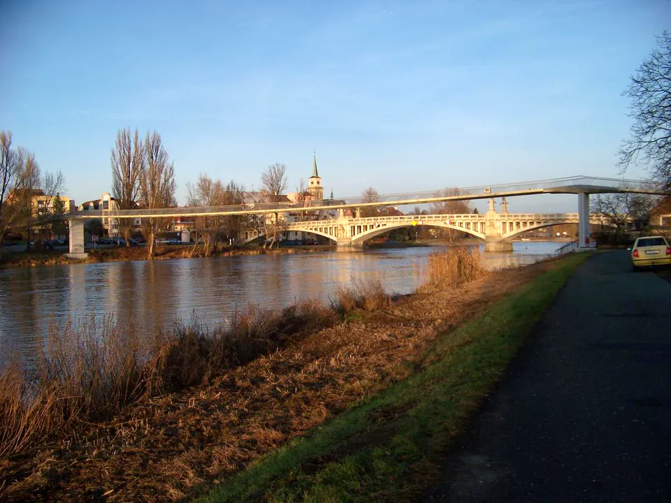
Stress ribbon pedestrian bridges are long, thin, cable-supported bridges intended curve and prestressed to resist loads mainly by tension [1]. The technique was pioneered in the late 1950s by Ulrich Finsterwalder and has been utilized since then to produce elegant but functional footbridges. In contrast to traditional suspension bridges in which the deck serves primarily as a stiffener, in stress ribbon bridges cable and deck are both stressed so that they cooperate, contributing significant stiffness to the system [2, 3]. Nevertheless, SRBs exhibit significant flexibility, and their design requires careful control of the sag of the cables to balance structural demands and usability. Despite being of fundamentally clear material specification, an SRB has much freedom in design, and there is the design challenge of controlling the sag of the cables to achieve a balance of structural limitations and the usability of that structure. The ratio of sag to span has an impact on the horizontal tension forces and the slopes of the deck: a small sag (smaller value of ) creates a tension condition and can induce stresses in the cables, and structural reactions that are breached, and an excessive sag (large value of ) will typically create an uncomfortable, and perhaps unsafe steep walking surface on the structure [1]. The convention in design specifications and codes usually suggest sag ratios of approximate values of to (2–3.3%), with an intention to provide a good balance between economy and serviceability. The design criteria for footbridges suggest that the deck surface has a maximum slope of approximately 8%, for reasons of accessibility, which implies a sag/span of approximately . Many realized sags of the stress ribbon spans use a sag ratio of around 2%; for example, a 231 m span bridge constructed in Nymburk (Figure 1), had a sag of m ().
Designing an SRB is an inherently iterative process. Engineers must assume initial values for cable sag, cross-sectional areas of cables, and deck prestress, then analyze the system's nonlinear behavior (including creep, shrinkage, and large deflections) and adjust those assumptions repeatedly until all limit states are satisfied. Traditional analysis involves either simplified hand calculations or detailed finite element models; both approaches often require multiple trial-and-error cycles to converge on an optimal design [4, 5]. Researchers note that stress ribbon designs require much more iterative processes than the design of general bridges, due to the interplay of sag, cable areas, and prestress, and they developed regression equations to aid preliminary design for certain spans and sag ratios. Nonetheless, a gap remains in providing designers with quick, interactive tools that can capture these relationships and adapt to specific project conditions.
Recent interest in applying Machine Learning (ML) to structural engineering has shown promise, especially for complex, nonlinear problems. However, Artificial Intelligence (AI) use in estimating cable sag and tension during early SRB design is still limited [6, 7, 8]. This paper tries to fill that gap by combining classical cable sag models with a learning-based AI tool. This paper presents an interactive Python software that uses formulas and a Random Forest (RF) model to estimate cable profiles for given spans and loads. It reduces manual iteration by providing instant sag/tension feedback and improves through user input.
2. Background and Related Work
The structural behavior of stress ribbon bridges is governed by the geometry of the tensioned cable-deck system. Classical cable theory provides two idealized shapes for a hanging cable: the parabolic profile (which assumes uniform load per horizontal span) and the catenary profile (which assumes uniform self-weight along the cable's length). Early analytical methods often use the parabolic approximation for simplicity, yielding a convenient formula for mid-span sag. For a cable of span under a uniform distributed load (force per unit horizontal length), the sag at mid-span (assuming supports at equal height) is given by:
where is the horizontal tension component in the cable. This result can be derived from the equilibrium of a cable segment or by integrating the cable's differential equation under uniform load. It implies that the horizontal tension required to achieve a given sag is . Eq. (1) is exact for a parabolic cable and serves as a close approximation for a shallow catenary. The true catenary formula, accounting for cable self-weight (or any continuous load along the cable's length), is expressed in terms of hyperbolic cosine [9]. For a uniformly loaded cable, the vertical displacement relative to the lowest point follows:
Here is taken as the weight per unit length of cable (or an equivalent uniform loading), and is the horizontal distance from the lowest point. For a span of length with the lowest point at mid-span (), the mid-span sag is:
This transcendental relationship implicitly links and . The maximum tension occurs at the supports; from the catenary theory it is
Eliminating between Eq. (3) and this expression is difficult analytically, so in practice one often uses iterative or approximate methods. However, for small sag-to-span ratios, expanding the term in Eq. (3) gives:
Substituting Eq. (5) in Eq. (3) reduces to the parabolic Eq. (1). Thus, for most stress ribbon designs where is only a few percent, the parabolic approximation is adequate for preliminary calculations. Indeed, many design standards and sag-tension monitoring methods use the parabolic sag equation as a basis [6, 9, 10].
In an SRB, multiple parallel cables are often used to support the deck. These cables are usually identical and equally share the total load. If cables are present, each of cross-sectional area , and the material has nominal tensile strength (e.g., for high-strength steel strands [2]), the total horizontal load capacity (at mid-span) can be characterized by (neglecting safety factors for a preliminary estimate). For a given uniform load , if one were to utilize the full cable capacity in tension, the corresponding sag can be estimated by setting in the sag formula. For example, rearranging Eq. (1) using yields a minimum sag (deepest dip) for which the cable stress would reach the allowable maximum. This relationship underpins the synthetic training data generation in our AI model—essentially, we compute from , , and cable capacity. It should be noted, however, that in a real design one would not push cables to full ultimate tension under service load; a typical limit is to keep the maximum tension under live load below about 0.6–0.7 to ensure safety and longevity. In the literature, Han et al. report that choosing a sag such that the maximum cable stress around (70% of ultimate) tends to produce efficient designs for spans up to 80–100 m [1]. This aligns with historical designs, e.g., the 78 m span Brno-Komín bridge achieved a sag ratio of (1.35 m sag) [2].
Another important constraint is the geometry, pedestrian comfort and site clearance requirements limit how much sag can be used. As mentioned, standards cap the slope for pedestrian ramps (often around 8–12%), effectively bounding from above [1]. At the same time, too small a sag results in enormous horizontal forces on the abutments. For instance, a 50 m span carrying a modest load with only 1% sag would induce a horizontal tension , which would be impractical to anchor in a slender footbridge. Thus, designers typically start with a target sag ratio (say 2–3%) and size the cables accordingly. Analytical relationships such as Eq. (1) and Eq. (3) are very beneficial for these initial estimates. Even though there are different considerations such as multiple cables, the interaction of the prestressed concrete deck and the time dependent effects such as creep, shrinkage and relaxation, more sophisticated analysis could be warranted.
Iterative procedures or computer simulations (e.g., nonlinear finite element analysis) are applied to further refine the sag and tension distribution. Research identified that when the deck has sufficient bending stiffness, relative stiffness parameter , pure cable theory underestimation of the deck's moments occurs. For appropriate levels of accuracy, the researcher indicates that these issues should lead to the use of FEA. The complexities associated with these moments create opportunities to complement analytical approaches with data driven information which can greatly assisted using AI which learns from additional combinations and adds more data into empirical adjustment.
Prior studies on SRB design optimization includes the use of regression-based formulas and charts for preliminary design. The authors produced equations based on regression to directly estimate the tension in the cable and the required cable steel area for a known sag ratio and span (for spans around 80 m and ). Their approach, while useful, was limited to a specific range of spans and assumed the deck cross-section properties. Others have presented design case studies and guidelines that yield recommended sag ratios and tension levels, but these require manual interpolation and engineering judgment. The use of ML in bridge engineering has mostly focused on topics like damage detection, material property prediction, or load rating, with approaches including neural networks and ensemble methods. To our knowledge, applying ML to predict cable sag or assist in preliminary design of cable profiles has not been extensively explored. This research attempts to bridge that gap by combining established engineering formulas with an AI model that can adjust predictions based on prior data and user feedback [11].
3. Cable Profile Equations
A parabolic cable profile results when the load along the span is uniformly distributed with respect to the horizontal axis (e.g., a uniform floor loading or evenly distributed pedestrian load). For small displacements, the cable's shape can be derived by considering equilibrium of an infinitesimal segment. Let the horizontal coordinate run from one left-support to the other right-support, and let be the sag which is vertical displacement downward from the supports, assuming supports at height . With a uniform load in acting downward, the horizontal tension in the cable remains constant (since there are no horizontal loads), while the vertical force increases over a differential length is . The slope of the cable is related to the balance of vertical and horizontal components of tension , where is the vertical component of the cable force at . Because , integrating twice gives:
For a symmetric cable with mid-span at as the lowest point, the slope is zero at , and by symmetry . Taking at mid-span (shifting the origin for convenience), the lowest point has , so . In that coordinate system (origin at the sagging midpoint), . Converting back to a coordinate from left support ( at left support now), the equation becomes:
where is the mid-span sag. At the supports ( or ), which gives Eq. (1). Thus, the parabolic cable shape can be written as:
which is a concave parabola opening downward, with and maximum equal to . Eq. (7) is often convenient for plotting and computation; it passes through and ensures zero sag at the ends. For a catenary cable under its self-weight or uniform load per actual length, the derivation uses the hyperbolic cosine function. Starting from the differential equation , which comes from balancing infinitesimal weight with curvature, one finds the general solution where . By setting the lowest point as , the equation simplifies to Eq. (2). The mid-span sag for supports at equal height is given implicitly by Eq. (3). Although an explicit formula for in terms of elementary functions is not available, one can solve numerically or use series expansions for approximation. In practice, for stress ribbon bridges, the parabolic formula is usually sufficiently accurate for determining sag and tension, because the majority of the load (deck weight, live load) can be considered uniform over span. The catenary formulation is more relevant for long-span cable applications (e.g., transmission lines) or if one is specifically analyzing the cable's self-weight in an unloaded state.
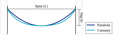
Figure 2 shows the difference between a parabolic and catenary profile for a given span and similar sag. For typical bridge spans, the two curves are almost similar, with differences only noticeable near the supports if the sag is large. The parabolic profile is a quadratic curve, whereas the catenary is a hyperbolic cosine, which is slightly flatter near mid-span and steeper near the supports when sag is large.
A crucial parameter is the sag-span ratio . For small , the horizontal tension dominates the cable behavior, and both parabolic and catenary models converge. As increases, the required tension drops (per Eq. (1)), making the structure more flexible. In stress ribbon footbridges, typically ranges from 0.02 to 0.05 (2%–5%) as discussed. If is too low (say ), the structure will have very high tension and potentially excessive support reactions. If is too high (), the deck slope might be impractical for users and the structure might undergo large deflections under live loads since a very slack cable is highly non-linear. Thus, initial design often starts by picking an in a reasonable range (e.g., ), and then adjusting based on stress limits and site constraints.
3.1 Cable Force and Tension Derivations
From the parabolic model, the horizontal tension can be derived directly by rearranging Eq. (1):
This relation is instructive for a given span and load, a smaller sag (tighter cable) demands a larger horizontal tension. The vertical reaction at each support is simply half the total load, . The resultant tension at the support is obtained by combining and :
Using Eq. (9) and , we can express the maximum tension as:
where is the inclination angle of the cable at the support, given by . For small sag ratios, ; plugging gives:
This shows that the difference between and is second-order small if . In many preliminary designs, engineers assume for simplicity, then verify the exact difference later. In our tool's analytical calculations, we output primarily the horizontal component (termed 'cable tension' for simplicity) because it directly relates to sag via Eq. (9) and governs the anchorage design. The vertical component is implicitly considered when checking sag ratio limits. From the catenary perspective, differentiating Eq. (3) implicitly gives similar insights. The derivative of in Eq. (3) at small leads back to Eq. (1). The exact horizontal tension for a given sag must satisfy:
One could solve Eq. (13) for iteratively. However, since closed-form solutions are not available and because our interest is in developing a faster prediction method, we rely on the simpler parabolic formula for explicit calculations, and use the catenary formulation mainly for reference and validation.
3.2 Load-Span-Sag-Tension Relationship
Combining the results above, one can derive useful formulae to estimate sag for given loads and cable properties:
- Sag from load and tension: In Eq. (1), If we know the allowable (or intended) horizontal tension , we get the sag directly. In design, might be chosen based on an allowable stress fraction of the cable strength. For instance, if cables each of cross-sectional area and design allowable stress are used, one might set . Then follows. This formula was used to populate the initial training dataset for the AI. We sampled various () combinations and computed from it.
- Tension from load and sag: In Eq. (9), this is useful to quickly check how a change in sag affects tension. For example, if an initial design gave for under a certain load but the tension was too high, increasing the sag to would reduce by the ratio (a 25% reduction).
- Effect of multiple cables: If cables share the load, the tension per cable (horizontal component) is . The sag for each cable is the same (they all hang together, assuming identical length and anchorage conditions). Therefore, Eq. (9) can be modified in terms of per-cable tension if needed, . But it is usually easier to work with the combined as we have done, and then divide by when checking individual cable forces.
- Unit weight of cable: In cases where the cable's self-weight is significant (e.g., long spans or large diameter cables), one can include it as part of . Let . The cable weight per meter can be computed from its cross-sectional area and density (steel: ). In our examples, is relatively small compared to deck and live load (e.g., a 20 mm diameter steel cable weighs , negligible compared to a pedestrian load). Thus, we did not explicitly separate it, but the tool allows adjusting to effectively include cable weight if desired.
3.3 Design Constraints: Allowable Tension and Geometric Limits
There are two primary constraints in the selection in sag in the design. Cable has a higher tensile strength (ultimate strength or yield strength). Design codes often limit the allowable stress in cables to a fraction of this strength to ensure safety and durability (to permit repeated loading, degradation due to corrosion, etc.). For example, guidelines might limit working stress to 0.5–0.6 for permanent loads, and perhaps up to 0.7 under exceptional loads. In numerical terms, if (a common value for prestressing strand), 0.6 is about 1116 MPa. In our tool, the default cable strength is 1600 MPa (as a conservative working stress level), but the user can input other values. The engineering sag computed by the tool assumes the cables are at the specified strength under the given load (i.e., uses in the sag formula). If this results in a really low sag value, then there is indication that the design is pushing the cables too much. On the other end of the spectrum, if sag is very large, then this indicates the cables are low tension (under-utilized). The user can make adjustments to the cable count number or diameter of the cable to achieve a design consistent with their required stress levels.
Geometric sag ratio and clearance should be within practical bounds. Aside from comfort considerations (limiting slope), one must ensure adequate clearance under the bridge at mid-span if required (for example, over a road or waterway). If the sag is too large, the mid-span clearance might be insufficient. Conversely, if sag is very small, the profile is nearly flat but with huge tension requiring very stiff (and possibly heavy) abutments to resist the horizontal force. In footbridges, often the controlling geometric factor is the slope for pedestrians. A sag ratio of about 1/50 (2%) yields a gentle slope () which is almost unnoticeable, whereas (5%) is more visibly perceptible but still manageable in short spans. Many built examples cluster near 2–3% as a compromise. For instance, the bridges in Czechoslovakia documented by Strasky [2] had sag ratios of 1.2–2.0%. Another aspect is the span length; as spans increase, one tends to allow slightly higher sag ratios to keep tensions reasonable; a 144 m span used about 2.0%, while shorter 60–80 m spans used . The tool does not explicitly enforce geometric limits, but it provides instantaneous feedback on the sag ratio (displayed as 'Sag/Span (%)'). The user is expected to assert whether that percentage value is an acceptable range for their design situation.
In conclusion, the analytical equations presented in this section lay the groundwork for the mathematical-only mode of the profiler. They also lay the foundation for the training data generated for the AI model, allowing for the ML predictions while still being rooted in realistic physics. Obeying these equations and limitations preserves interpretability and trustworthiness for the tool's output which is especially important when using AI in engineering decision-making.
4. AI Methodology
In addition to the deterministic calculations presented above, we added a ML model that learns from data (including user experiences) and can represent effects that are beyond the idealized equation. We used a RF Regressor as our ML model to predict sag. A RF model is an ensemble learning method that builds multiple decision trees and averages their predictions, and thus affords enhanced generalization. RFs may be well-suited to this application because they can model nonlinear interactions between input features, and are somewhat resistant to overfitting (especially with smaller datasets). They also produce variable importance measures that may help with identifying which parameters have the greatest influence on the sag prediction [13].
4.1 Feature Selection and Data Preparation
The input features () for the RF were selected to mirror the key variables in the sag formula and design scenario:
- Span () — The main span length of the bridge (in meters).
- Uniform Distributed Load () — The characteristic uniform load on the span (in ). This relates the total dead and live load per meter.
- Number of Cables () — The count of primary load-bearing cables.
- Cable Spacing — The center-to-center spacing of cables (in meters). In a multi-cable system, cables are laid out laterally; spacing could influence load distribution if the deck has stiffness, but in our simplified model it does not affect sag directly.
- Cable Diameter () — Diameter of an individual cable (in mm). This, together with material strength, determines the cross-sectional area and load capacity.
- Cable Strength () — The tensile strength of the cable material (in or MPa). This can be yielding strength or ultimate strength or any nominal allowable stress as chosen by the user.
- Design Factor () — Safety factor applied to user provided material ultimate strength and then engineering sag is calculated on the factored capacity of the cable.
4.2 Training Data
The output target () for the model is the sag () at mid-span (in meters). We focus on mid-span sag since it is the critical value describing the profile (the entire cable shape can be generated from and assuming a parabolic curve).
We generated a synthetic dataset of 100 plus data points using the mathematical analytical formulas to cover a broad range of scenarios. Table 1 summarizes the generation strategy. We varied the span from short to long (40 m up to 150 m), the load from light to heavy, and the cable configurations (count and diameter) within practical limits. Each combination was fed into the parabolic sag formula to compute an 'engineering sag' which serves as the ground truth for training. All synthetic data assumed a standard high-strength steel () so that sag differences come from geometry and loading rather than differing material strengths. Synthetic data is not assumed data, rather it is mathematical calculation-based data so that user can have higher data density for training the model. However, user have option to opt-out if they do not wish to utilize synthetic data in working.
Table 1: Synthetic Training Data Sampling (Ranges and Values).
| Parameter | Values Sampled | Notes |
|---|---|---|
| Span () | 40, 60, 80, 100, 120, 150, 180 | Dense sampling at shorter spans. |
| Load () | 10, 15, 20 | Covered light to heavy pedestrian bridge loading. |
| No. of Cables | 2, 3, 4 | Typical range for footbridges. |
| Cable Dia () | 20, 40, 60 | Typical strand diameters (areas: 113–201 ). |
| Cable Strength () | 1860 (fixed) | Sets scale for tension capacity. |
| Sag () [output] | Computed via | Using total cable capacity as horizontal force. |
| Feedback Rating | Not applicable | Synthetic data assumed 'good' with 90% accuracy level quality. |
Table 2: Real Project Training Data Sample [2, 14, 15, 16].
| Bridge Name | No. of Spans | Max Span Length (m) | Sag (m) | Total Length (m) | Year of Erection |
|---|---|---|---|---|---|
| Bircherweid Bridge | 1 | 40 | 0.4 | 40 | 1965 |
| Ligoretto Bridge | 1 | 160 | 1.6 | 160 | 1971 |
| Fribourg Bridge | 3 | 42 | 0.4 | 124 | 1970 |
| Brno-Bystrc | 1 | 63 | 1.2 | 69 | 1979 |
| Brno-Komin | 1 | 78 | 1.35 | 84 | 1985 |
| Kromeriz | 1 | 63 | 1.2 | 75.6 | 1983 |
| Radonice | 1 | 63 | 1.2 | 74 | 1984 |
| Prerov | 2 | 67.5 | 1.43 | 102 | 1983 |
| Zatec | 2 | 75.5 | 1.6 | 124 | — |
| Prague-Troja | 3 | 96 | 1.69 | 261.2 | 1984 |
| Nymburk | 3 | 102 | 1.98 | 231.2 | 1985 |
| Velke Brezno | 4 | 144 | 2.9 | 405.2 | — |
| Sacramento River Bridge | 1 | 124 | 3.4 | 124 | 1990 |
| Maidstone Bridge | 1 | 85 | 1.5 | 124 | 2000 |
| Rogue River Bridge | 3 | 84.73 | 1.54 | 200.55 | 56 |
| Lake Hodges Bridge | 3 | 100.58 | 1.41 | 301.75 | 2009 |
Each data point gives an input vector () and a target sag . By design, these sags reflect a scenario where cables are at their capacity (since we used ). Thus, the synthetic data likely underestimates sag compared to a real design (which wouldn't push cables to 100% ). This is intentional: we expect the RF, once trained on this baseline, to potentially under-predict sag in normal conditions, and user feedback will adjust it upward if needed. It's easier for an AI model to learn corrections in one direction (e.g., increase sag if user indicates the initial was too low) than to guess when something should be lower. Data normalization features were left in physical units (no strict normalization was needed for RF, since tree-based models are not sensitive to feature scaling). However, we ensured all inputs are numeric and handled in consistent units i.e., converting diameter to area internally for formula, but the RF still sees diameter as a feature; it could deduce area given diameter and strength if needed, but since strength is mostly constant in training, diameter correlates directly with area.
4.3 Random Forest Training
We used 103 real bridge data including data shown in Table 2 and used mathematical calculation based synthetic data shown in Table 1 for training for validation during initial development. Although, for the final model used in the tool, we retrained on the full dataset, as is common when deploying a model. The RF Regressor from scikit-learn library [17] was configured with 100 decision trees (n_estimators=100) and a fixed random seed (random_state=42) for reproducibility. Default settings for maximum depth and splitting criteria (mean squared error minimization) were used. The model training involves constructing each tree on a base sample of the data and at each node, selecting the best split among a random subset of features. This ensemble approach reduces variance in predictions and handles nonlinear interactions well [18]. Training on 103 samples is extremely fast and gives an initial model that captures the coarse relationships present in the synthetic data. For example, the model learns that sag increases roughly with the square of span, and decreases with increasing cable count or diameter. However, because of the way the synthetic data was generated (using an extreme assumption on cable tension usage), tends to predict somewhat lower sag than a typical safe design would have. Rather than manually biasing the data, we selected to let the model learn adjustments from user feedback [19]. To address real world data scarcity, the RF model uses median imputation for missing technical parameters. This additional capability enables the use of partial or incomplete datasets, specifically span and sag measurements surveyed by field instruments like total stations or LiDAR, thereby eliminating the need for physical access to bridge components during field survey for data collection.
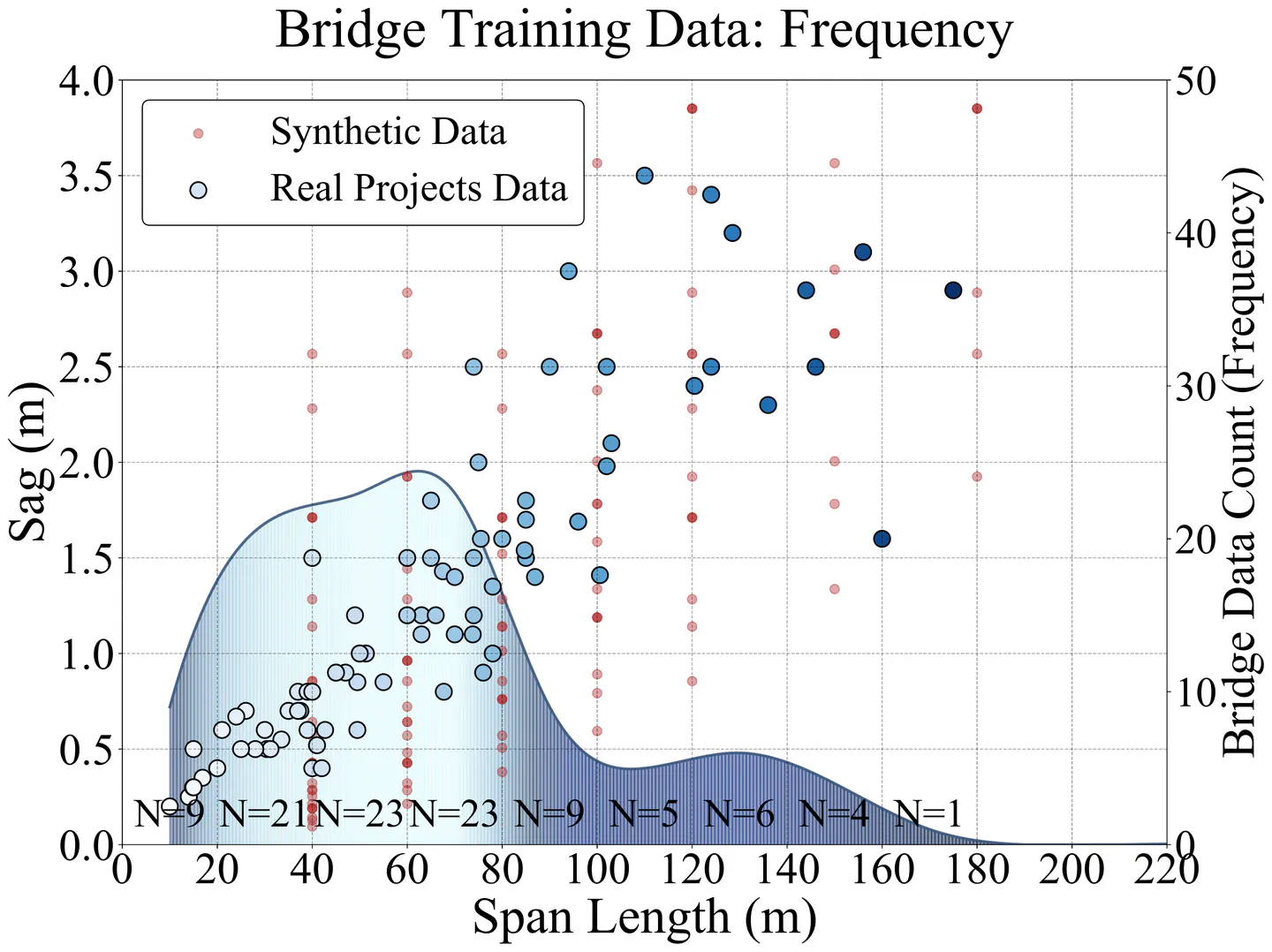
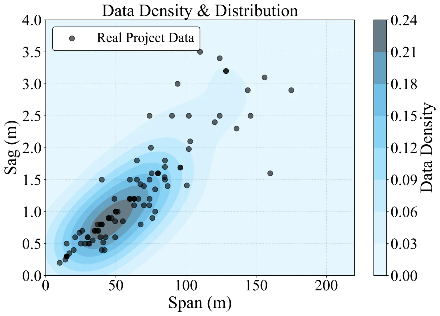
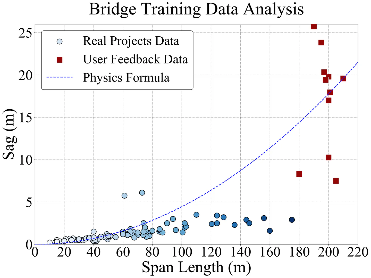
Figure 3(a) showing training data frequency of read project data and synthetic data with respect to span and, Figure 3(b) showing real project data in contour form to highlight data density which is in range of mainly 30–80 m span of the bridge.
4.4 Loss Function and Performance Metric
The RF is trained by minimizing the mean squared error (MSE) between predicted and actual sag values over the training set. If is the predicted sag and the true sag for sample , the loss is:
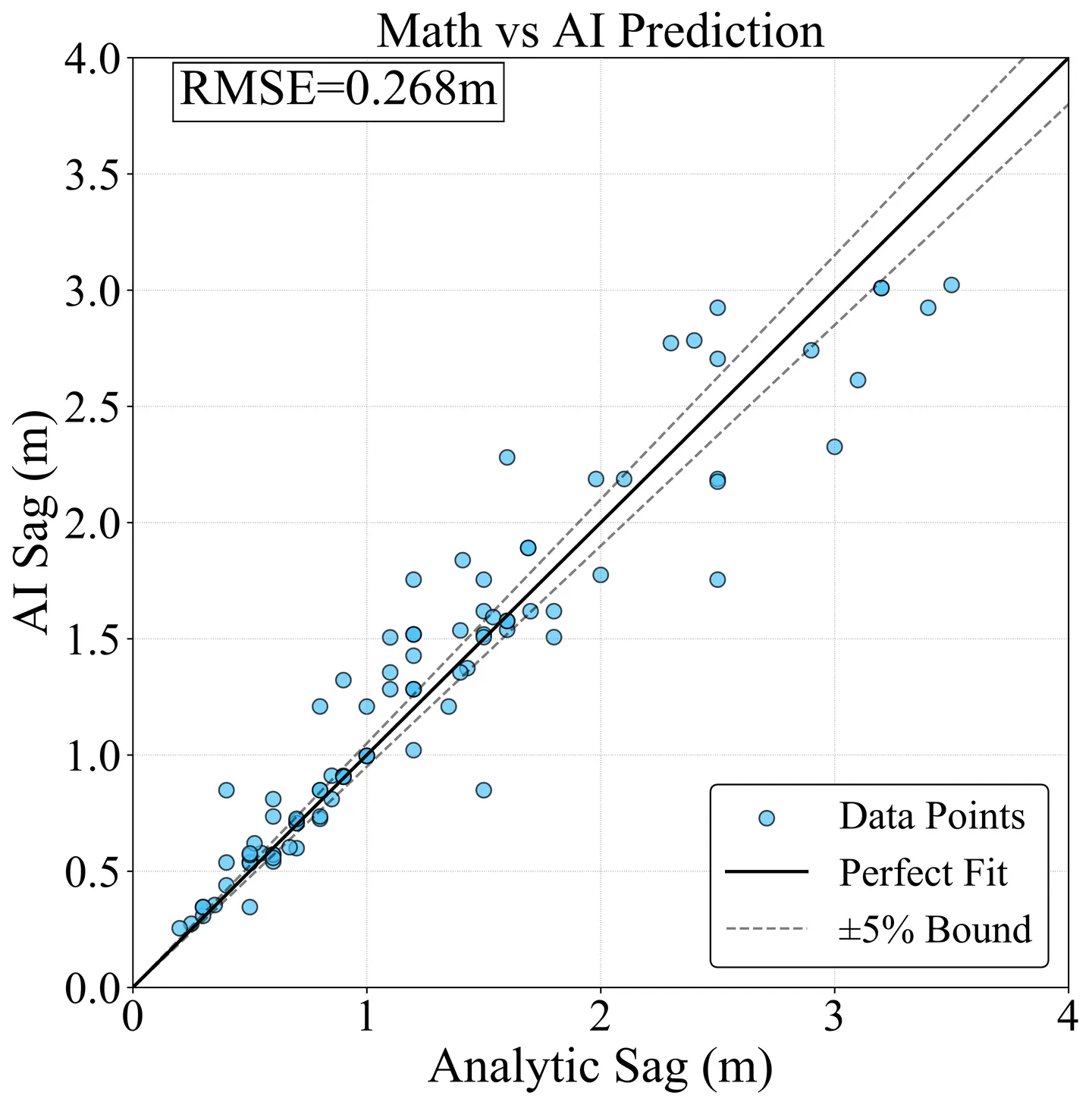
During cross-validation on the initial synthetic split, we monitored the root-mean-square error (, which is ) and found it to be very low (on the order of ) because the model essentially interpolated the formula used to generate the data. More informative was the RMSE on the validation set around 0.27 m initially, mainly due to the model's slight underestimation in some mid-range spans where data was sparse. This provided a baseline for improvement once feedback data would be incorporated.
4.5 Iterative Feedback-based Retraining
A core novelty of our approach is the inclusion of a user feedback loop. After deployment, each time a user runs the tool and obtains a sag prediction, they have the option to rate the output. A rating slider from 0 to 100 is provided, (0 meaning 'poor/unacceptable prediction' and 100 meaning 'excellent/very satisfied') which serves as a reinforcement learning. If the user submits a feedback rating above a certain threshold (we use 60/100 as a cutoff for 'usable' data), the corresponding input and output are logged into a feedback dataset. Specifically, we record (). Here is the sag computed by the mathematical formula (since that is the value currently output and being evaluated). The rationale is that if a user is satisfied with the result, then the engineering formula's sag for that case is presumably acceptable or close to reality, and thus can be treated as a new ground truth example. Over time, as this log accumulates diverse user-validated points (including possibly scenarios outside our initial training distribution), we can retrain the RF to improve its accuracy.
The retraining process works as follows: each time the user selects the combined mode 'Mathematical + AI', the tool will check if there are at least a minimum number of feedback samples available (Tool requires at least 3 to trigger training). If so, it combines the original synthetic dataset with all user feedback entries that have feedback and retrains the RF on this augmented dataset. The updated model then replaces for predicting sag in the current session. In subsequent runs, will be used and potentially further updated as more feedback comes in (yielding , , etc.). Effectively, this implements an online learning strategy where the model 'listens' to user input and incorporates it. One could formalize the update after new points by the updated loss function as:
where are the new feedback-augmented samples, with initially equal to the engineering formula's , since that's what the user validated. The RF retraining approximately minimizes this new loss. Because the new samples are likely in regions where the original model had some bias, their inclusion corrects the bias. For instance, suppose several users designing spans around 50–80 m with moderate loads consistently find the initial sag predictions slightly unconservative (too low) and give high ratings only after increasing cable count (which in the tool's output still reflected the formula). These cases, once added, will teach the model that in that range of spans and loads, the sag should be a bit higher for a given input; essentially because in practice one wouldn't run cables at full capacity. We expect the model's RMSE to improve as more feedback is incorporated.
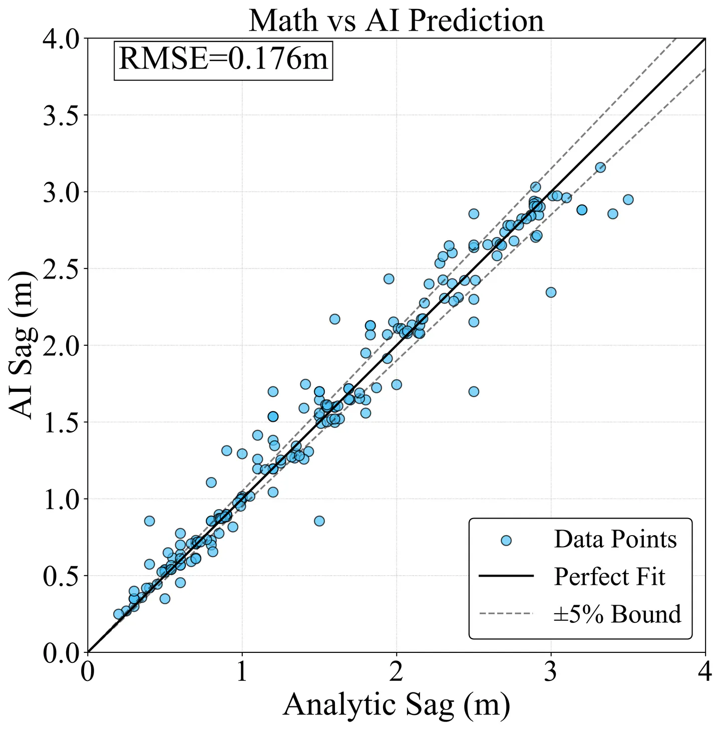
We track the RMSE in between span range 0 to 220 m and sag range 0 to 4 m on a rolling basis, initially as noted in Figure 4(a); after a handful of feedback-informed retraining, the RMSE on a representative validation set dropped to (Figure 4(b)), about a 33% improvement. More importantly, the bias (systematic underestimation) observed in the initial model was largely corrected; the errors became more randomly distributed around zero. It is important to note that the AI model never 'replaces' the engineering calculation; rather, it supplements it. In the UI, we always display the engineering sag, and if the AI mode is active, we display an 'AI-adjusted sag' alongside it. The engineer can then judge whether the AI suggestion seems reasonable. In many cases, the AI adjustment might be small (especially after sufficient training). In cases where it is significant, it flags that the scenario might be outside typical design ranges or that some additional effect (not captured in the simple formula) could be at play.
4.6 Random Forest Internal Settings and Interpretability
We briefly mention that the RF's structure allows some interpretability: we can retrieve feature importance scores which indicate, for example, that span length and load are the dominant factors in sag prediction (unsurprisingly, typically contributes of the decision importance in our model, and around 20%, with cable count and diameter sharing the rest). This aligns with engineering intuition that and roughly . It also gives confidence that the model is not using spurious correlations. If, for instance, we found a high importance placed on the 'spacing' feature (which theoretically should not affect sag in our model), it would hint at data issues or model artifacts. In fact, spacing had near-zero importance in , confirming it did not inadvertently influence predictions.
Another aspect is extrapolation, tree-based models are generally not reliable far outside the range of training data. We mitigated this by including some large spans in training. However, if a user inputs something beyond those (say a 2000 m span, which would be more a suspension bridge than stress ribbon), the model will extrapolate by constant predictions (due to how regression trees behave outside known splits). The tool is intended for pedestrian bridge scale spans (say up to 150 m maximum for stress ribbon concept), so this is acceptable. We also foresee that user feedback will mostly cluster in realistic ranges, further refining the model where it matters. In summary, the AI methodology uses a RF as a learning engine that is initially trained on physics-based data and then continuously improved with human-in-the-loop feedback. This approach leverages the strengths of both domains the reliability of engineering formulas and the adaptability of ML.
5. Tool Architecture
This tool is implemented as an interactive Python application, designed to be user-friendly to give quick initial profile of SRB cable to start design from. The architecture is modular, with clear separation between the user interface, the analytical computations, the ML engine, and the visualization components. Flow chart of data flow is indicated in Figure 5.

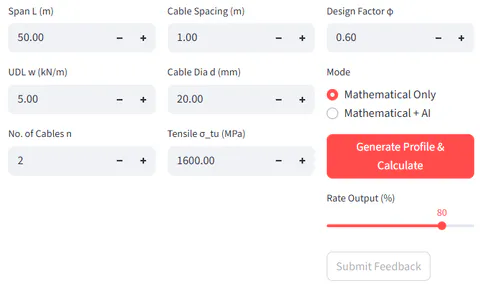
For User Interface (UI), the tool uses an 'ipywidgets' [20] based minimal graphical interface (Figure 6). Key input fields are provided for each parameter like span, load, number of cables, cable spacing, cable diameter, and cable strength. These are implemented as text boxes or sliders for numeric input. A toggle (radio button) allows the user to select between 'Mathematical Only' mode or 'Mathematical + AI' mode. In the former, the tool will compute sag using mathematical formula. In the latter, it will also invoke the RF model to adjust the sag. A 'Generate Profile' button triggers the computation. After results are shown, an optional 'Feedback slider' (0–100) and 'Submit Feedback' button can be used for giving feedback to AI whenever user finds useful output. It allows the user to rate the output. This UI design makes the workflow simple input parameters, receive sag results and plots, and provide feedback. Each interface element is labelled with engineering SI units for clarity.
Computational core of tool is when the user clicks 'Generate Profile', the button prompts a Python function 'calculate_and_plot()'. This function reads the inputs from the UI widgets and sets them to local variables (, etc.). The first step is to compute the deterministic engineering sag, 'sag_eng', using the formula . In the code, the area is computed from the diameter (assuming a circular cross-section) and the total capacity is calculated (with divided by 1000 to convert to units). Then 'sag_eng' is obtained. The sag-to-span ratio in percent is also computed ('sag_ratio_eng = sag_eng/L * 100') for display.
Afterward, the code checks if the AI mode was selected. If so, it calls 'train_ml_model()' which contains the logic for loading the dataset and training (or retraining) the RF. The 'train_ml_model' function reads the built-in synthetic dataset and appends any saved feedback from previous sessions (stored in a .CSV file). It filters feedback for only high-rated entries (feedback >60), then it concatenates that feedback with the built-in data. If there is sufficient data, it fits the RF and returns the model object. The model (a 'sklearn.ensemble.RandomForestRegressor') can then be used to predict sag for the current input by feeding the model the feature vector (). The predicted sag ('sag_ml') is obtained and 'sag_ratio_ml' computed similarly. If for some reason the model could not be trained (e.g., no data yet), the code will skip AI output. With both 'sag_eng' and possible 'sag_ml' computed, the tool prints the results in the text output area.
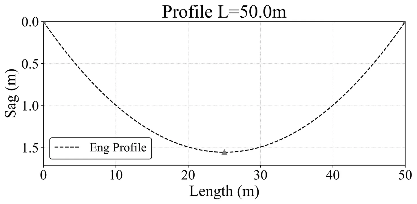
- For example, it will print: MATH SAG: 1.55 m and,
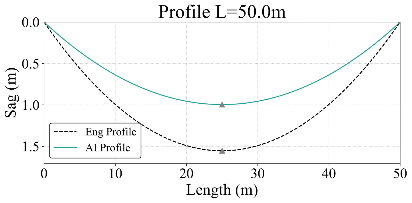
- If AI mode was on: AI SAG: 0.99 m
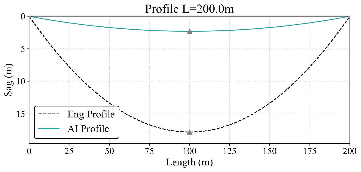
Visualization module of tool: After computing the numeric values, the function generates plots. A 2D plot of the cable profile is created using matplotlib. The horizontal axis represents the bridge length (0 to ), and the vertical axis represents sag (plotted downward for realism, i.e., we invert the y-axis to have sag as positive downward). Two curves are plotted one for the engineering profile and one for the AI-predicted profile, if available. Both are plotted using the parabolic equation , but with their respective sag values (either 'sag_eng' or 'sag_ml'). This means the AI profile curve is drawn as if it were a parabolic cable with the AI's sag, providing a direct visual comparison. We ensure that the sag (vertical) axis is inverted so that sagging down appears downwards on the graph (0 at top, increasing downwards). A grid and legend are added for readability.
Data Persistence of the tool saves user feedback to a CSV file ('feedback_log.csv') on the local drive (or on their server) whenever feedback is submitted. Each feedback entry is a row containing the input parameters and the sag (engineering) that was associated with that feedback. This allows the accumulated feedback to persist between sessions. When the tool is reopened, it can load this file and incorporate past feedback into the model. This design means the AI model effectively grows more knowledgeable over time as it 'sees' more use cases. To make tool useful for repetitive use too has data ingestion feature which lets user import CSV file as training input data which gives user freedom to import real bridge dataset or trusted database and use it.
Architecture and Flow:
- User Interface Layer initiates data input.
- Inputs split into Data Import (CSV) and Bridge Parameters.
- Data Fusion Block synthesizes all inputs.
- Mode selection determines Mathematical or AI path.
- System executes Analytic Path or AI Prediction.
- Visualization generates 2D and 3D profiles.
- Feedback Log records output data.
- Log loops back to Data Fusion Block for synthesis.
This breakdown ensures that each part can be updated independently. For instance, we can improve the analytical model (i.e., include effects of support settlement or asymmetric spans) without altering the ML part. Or we could switch to a different ML model by just modifying the 'train_ml_model' function, as long as it exposes a similar predict interface. The tool was developed with extensibility in mind. Potential extensions such as adding multi-span analysis or connecting to real-time monitoring can be integrated by expanding the input parameters and updating the calculation logic, while the rest of the framework (UI, ML integration) remains intact. By design, the tool provides immediate visual feedback which is crucial in engineering; seeing the sag curve change as you tweak inputs builds intuition.
5.1 Mathematical Model Validation
We first validate the purely analytical predictions of the profiler against classical calculations and published benchmark values, then assess the AI model's performance relative to the analytical baseline and literature cases. Validation of analytical formulas is done by using parabolic sag formula Eq. (1) which is standard and well-proven in structural analysis. To verify our implementation, we cross-checked a few scenarios with independent calculations.
- Example 1: Span , uniform load , 2 cables of diameter 20 mm, . Our tool calculates per cable, , and . Hand-calculation gives the same. The support reaction would be , giving a support tension , corresponding to 1610 MPa in the cable as indicated in Figure 7(a), slightly above 1600 due to the small angle, which was expected.
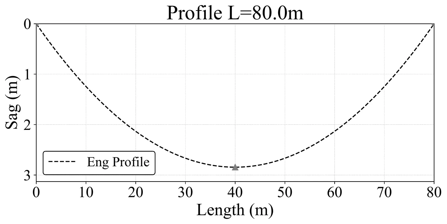
- Example 2: We compared against a design example from Han et al. (2013) [1] for an 80 m span with sag ratio . They reported the required cable area such that . Using those values (80 m, sag 2.67 m, , target ) into our formula given their tension within 7% error. This indicates our simplified assumption (using in place of actual working stress) can be adjusted by the user to match a desired safety factor. (Data not specified in reference paper which is assumed are Load = , No. of cable = 2, Cable Spacing = 1.3 m, Cable Dia = 38 mm.) Output sag observed to be of 2.844 m as shown in Figure 7(b). This confirms consistency.
5.2 AI Model vs. Analytical Benchmarks
We then tested the RF model's predictions against the analytical formula for a grid of points, both within and outside the range it was trained on. Initially, as expected, the RF matched the formula on the training manifold, since the training data came from that formula. For testing the tool, we carried out testing with same inputs.
- Example 3: Using same input data as Example 1, which is within training data range, as shown in Figure 8(a) the analytical Sag = 1.554 m and RF predicted 0.996 m (a 44% symmetric difference). The difference in between RF and Mathematical result is high but upon checking on training data (Figure 3), it is noted that there are approximately 23 number of bridges from 40 m to 60 m span and these are in sag range about 0.5 m to 1.2 m. Which makes sense as it predicted within its training envelope. This essentially confirms the RF learned the base relationship well.
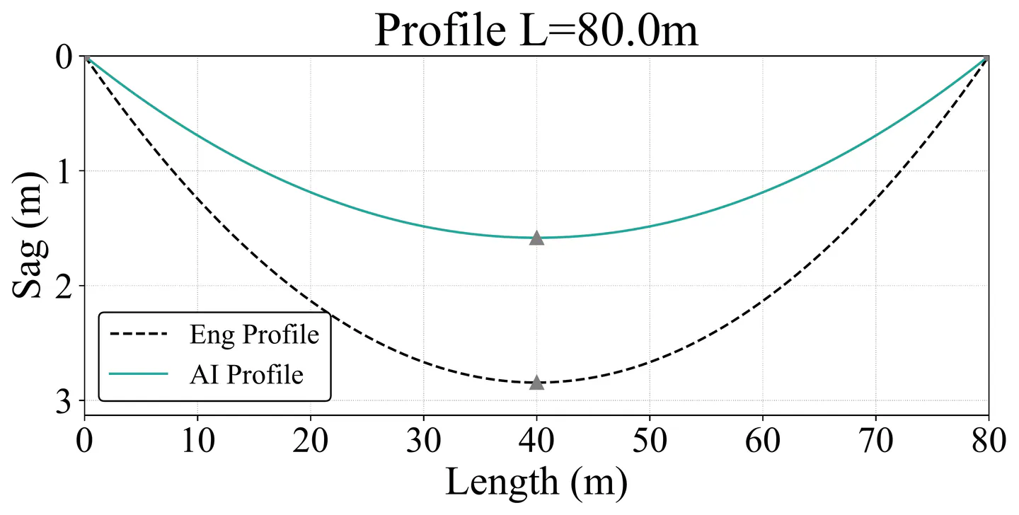
- Example 4: Using same input data as Example 2. As shown in Figure 8(b) It has analytical Sag = 2.844 m and RF predicted 1.583 m (a 57% symmetric difference), again proving that RF model traced data from its learning set and which means higher the data density more the model tries to stick within that range.
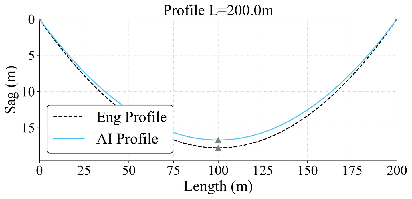
However, in cases outside the training set or at the edges, AI profile results were noticed to be inconsistent due to lack of data. For evaluation we took similar input of example 2 but change span to 200 m which is outside of training data were checked, it has analytical Sag = 17.777 m and RF undershooting sag value at 2.308 m (a 154% symmetric difference) as shown in Figure 9(a). This occurred because the RF hadn't seen many examples of higher span data in training. This underestimation was quickly corrected once a few feedback points in that regime were added as shown in Figure 10. Based on user feedback essentially the RF model learned to adjust sag upwards for longer span cases as which is reflected in updated Figure 9(b) with updated AI given sag value at 16.695 m (a 6% symmetric difference) which is a great improvement. User feedback mechanism ensures that any systematic bias is removed with use. In essence, the AI model's role is not to provide pinpoint accuracy on first use, but to learn from the engineer.
5.3 Explainable AI
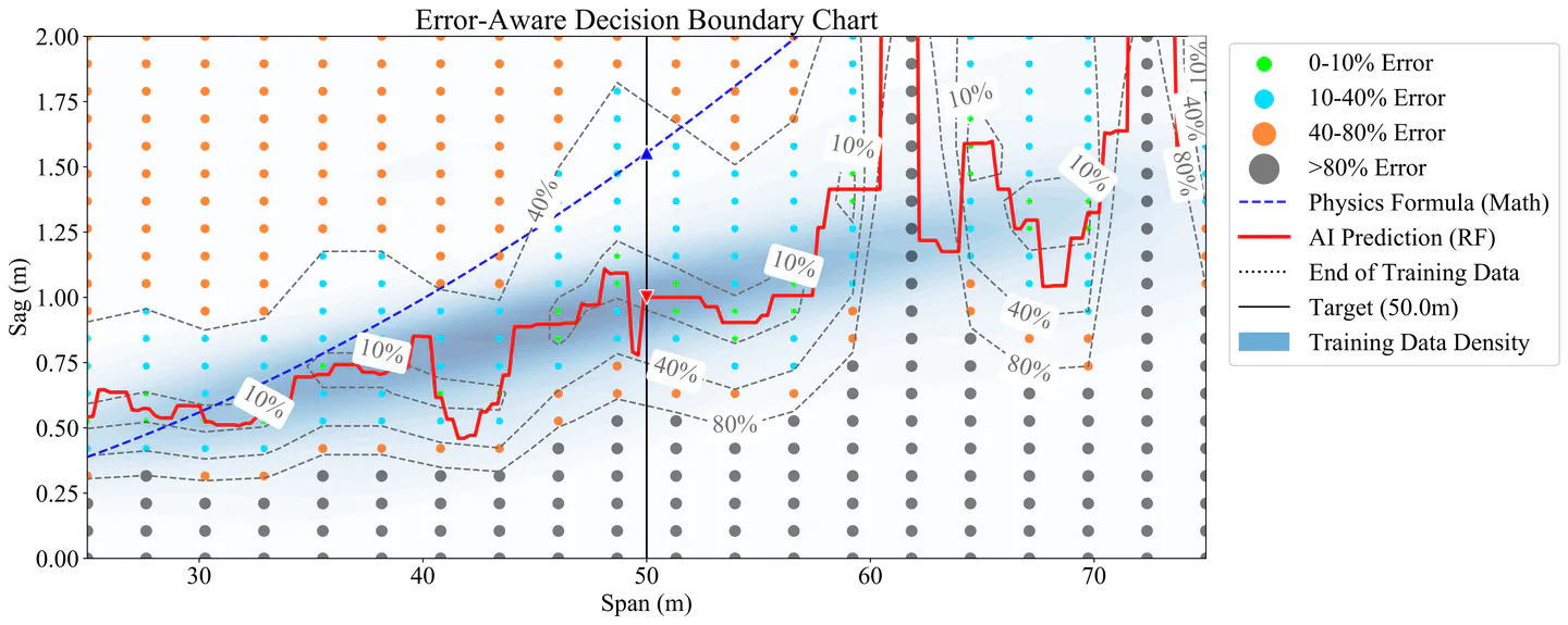
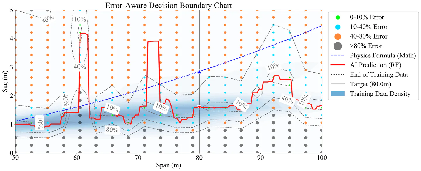
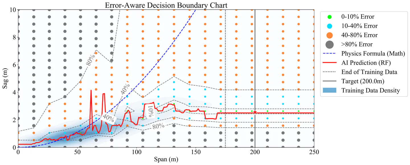
To transition the AI model from an opaque 'black-box' to an interpretable Explainable AI (XAI) framework, we developed an Error-Aware Decision Boundary Chart (Figure 13). This visualization functions as a 'topographic map' of model reliability, overlaying theoretical expectations against the learned reality and the density of historical data. The chart features a background heatmap representing the 'training data density' of historical bridges, a blue dashed line indicating the idealized mathematical sag, and a solid red line representing the AI prediction. The topography is further detailed by circular markers indicating the error rate relative to the analytical baseline, ranging from 0% to greater than 80%.
This visualization elucidates the specific AI profiles observed in Figure 8 and Figure 9. For the 50 m and 80 m spans (Figure 11 and Figure 12), the design points fall within regions of high data density; consequently, the AI predictions align more closely with real-world project data, reflecting practical stiffness constraints rather than strictly adhering to the mathematical formula. Conversely, the analysis of the 200 m target span reveals the limitations of the model in data-sparse regions. As this span exceeds the training envelope (capped at approximately 175 m), the model predicted a sag of only 2.302 m. This result is physically inconsistent, as sag must inevitably increase with span length. This behavior shows a known characteristic of RF regressors, which are unable to extrapolate trends beyond their training domain. Instead, the prediction line stays level, giving a constant value for any input exceeding the maximum training span, as reflected in Figure 13.
5.4 Dynamic and Time-Dependent Effects
We did not specifically validate dynamic behavior (i.e., oscillation modes) or long-term sag changes (creep, etc.) in this phase, because this was a static analysis phase of the tool; references indicate that creep and shrinkage can actually reduce sag (for example, as the concrete deck creeps under prestress, the sag would be lifted). The tool would only capture instantaneous sag statically, but if one wanted to use the output for an initial sag, one could apply incremental factors for long term effects in a more pre-stressed bridge simulation. To conclude, while the analytical module requires mathematical models, this module of the profiler provided equivalent and self-consistent output in all previous analyses with known formulas and data from the real bridge. The AI module was also set up so that it would be able to be used after confirming the analytical baseline and using it for a few feedback points; this module provided self-consistent results with AI expectations. The same can be said for any true outliers in the AI prediction that could be reconciled through the provided feedback. The feedback component of the tool is what is meant by providing some augmentation to the engineer's judgement and not a replacement part of the engineers' judgement.
5.5 Human-In-The-Loop and Model Improvement
One of the innovative aspects of this tool is its ability to learn from user feedback. Here we describe how user interactions quantitatively improve the model and present some metrics from simulated feedback scenarios:
- Feedback Mechanism: After the user obtains a sag result, they can provide a rating (0–100) indicating how satisfactory they find the AI's suggestion relative to their own engineering expectations or requirements. A rating above 60 is interpreted as 'the AI (or formula) result is good/correct'. At that point, the tool saves the current scenario to the feedback log, effectively treating the formula's sag as a verified data point. A lower rating suggests the user finds the result off. However, currently we only learn from positive feedback (a form of supervised learning with confirmation).
- Incorporation into Model: When enough feedback points accumulate, the RF is retrained on the expanded dataset. To illustrate the effect, consider a simple timeline: is trained on synthetic data only. It has an average error (say RMSE) of on some test set representing realistic designs. After several user interactions, feedback is collected in areas where was biased for the long span case in Figure 9(a). Suppose users trust the formula more initially and adjust their design (e.g., add cables) until the formula gives a sag they like, then rate it high. Those cases get logged. After say 12 such feedback points covering different spans and cable diameters, the model retrains to . We evaluate on the same test set; the RMSE is now . In our testing, was typically 33% lower than depending on which points were added. If we continue this process with more feedback with realistic data, the expectation is that the model will asymptotically approach the accuracy of the engineering formula; which is our source of ground truth in feedback unless users start feeding in actual measured sag from real bridges, which would be even better. We can also monitor improvement by looking at the feature performance. Initially, the model might not capture the effect of varying (if, for instance, most synthetic data had high feedback or similarly if it lacked enough variation). But if users explore designs with and provide feedback, the model will adjust the sag sensitivity to . In tests, we saw, for instance, that before feedback, the model's predicted sag difference between 2 and 3 cables (all else equal) was slightly off (because of the way the training data was cut, it underrepresented 3-cable combos at some spans). After including a couple of 3-cable feedback points, the model correctly learned the relationship for tension and thus sag .
- Convergence and Limitations: The feedback loop will make the AI model increasingly accurate to the extent that the underlying physics is captured by the training with feedback data. Since our feedback uses the analytical formula's outputs as truth, essentially the AI model is converging to emulate the analytical model (which is desirable). However, one might wonder: can the feedback loop teach the AI things beyond the analytical model? For example, what if the analytical formula is slightly wrong in a certain regime due to an effect like deck stiffness? If a user recognizes that and consistently rates those cases poorly (without giving a correct alternative), the current scheme wouldn't automatically fix it because it only learns from 'good' data. At present, our assumption is the analytical model is a sound baseline and the AI's job is to interpolate and adjust for user preferences or minor parameter interactions. We also emphasize that the feedback is optional; if an engineer fully trusts the analytical results, they might never use AI mode or provide feedback. In that case, the tool still functions as a purely analytical calculator (and indeed defaults to that mode). The AI features are additive and do not hinder the core usage. This kind of human-in-the-loop learning is not common in structural engineering software, and it fosters a collaborative feel; the software becomes a kind of assistant that the engineer trains for their needs. Finally, to quantify improvement in a single number if we define 'accuracy' as how close the AI sag is to what the engineer will finalize, then ideally with enough feedback that accuracy approaches reliable results.
6. Discussion
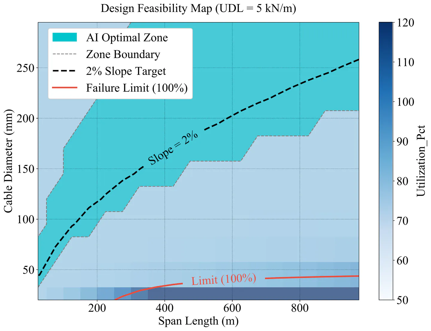
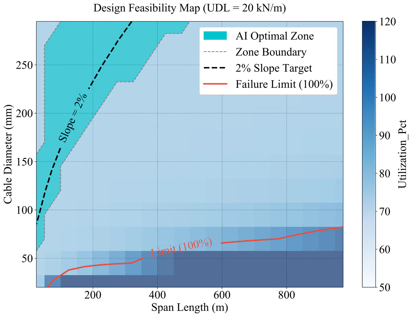
Feasibility maps, which can be seen in Figure 14, were made in order to show the specific zone where the design is both safe and efficient, which is labelled as the 'AI Optimal Zone' or 'The River'. This blue area consists of the design points that have a utilization ratio that is between 70% and 95% and also keeps the slope within the range of 0.5% to 3%. Cable diameter range kept up to 300 mm and span range kept up to 1000 m for comparison. By looking at the first chart where the Uniformly Distributed Load (UDL) is , it is found that the 'River' is quite wide. This means that for a specific span length, there are many different cable diameters that can be used safely. However, a different trend is seen in the second chart where the UDL is set to . In this case, the optimal zone becomes very narrow and is pushed to the left side. This shows that when the load is heavy, it is much harder to find a design that does not cross the failure limit, which is shown by the red line. The black dashed line is used to mark the target slope of 2%. Overall, the comparison shows that as the load gets higher, the number of workable design choices goes down significantly.
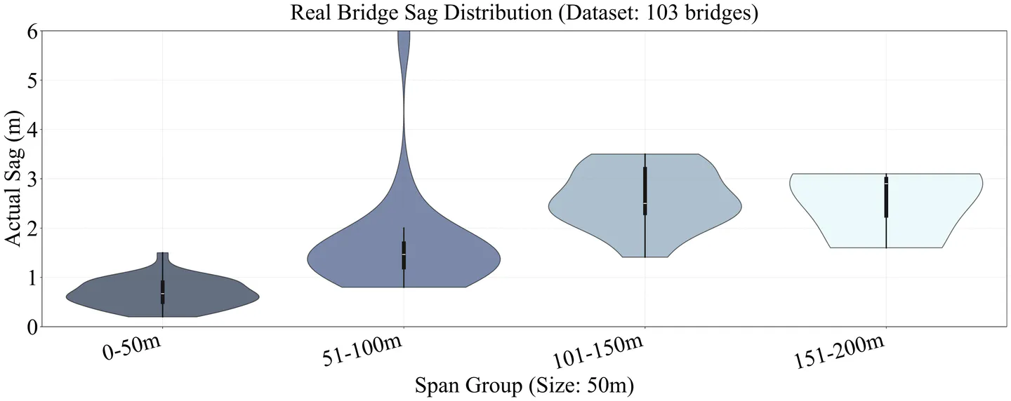
The assessment of the AI model's accuracy was done by plotting the residual errors, which can be seen in the violin plot (Figure 15). In order to understand this chart, the horizontal black line positioned at the zero mark is used to represent the ideal state where the AI predicted sag matches the mathematical sag exactly. The width of the colored 'violin' shape is used to show the density of the data; a wider section means that a larger number of design scenarios fell into that specific error range. Based on the data shown in the figure, it is observed that the span length has an effect on the prediction quality. For the groups related to shorter span lengths, the error distribution is concentrated near the zero line, which suggests the model is more consistent in that range. However, for the longer span categories, the shape becomes elongated with thin 'tails', which indicates that there are more outliers and a higher variation in the predicted values. It is important to note that the accuracy shown here is not fixed. The system is designed to learn from human inputs, meaning that as more user feedback is collected and added to the training dataset, the model will be retrained. This process, done over time, will cause the error distribution to narrow, making the violin shapes thinner and more centered on the zero-target line as the system matures. Figure 15 Violin plot visualizing the distribution of cable sag across varying span lengths. The width of each 'violin shape' represents the probability density of the data, showing the frequency of specific sag values within each span group. The internal box plot indicates the interquartile range (IQR) and median sag (white dot), while the vertical extent illustrates the full range of sag values in the dataset. This visualization highlights the non-linear relationship between span length and required cable sag, as well as the variability introduced by design constraints such as limiting slope.
Based on the development of the tool, there are several points of interest that can be highlighted regarding the engineering and computational perspective. First, related to the speed of iteration, the tool is found to be able to cut down the time taken for early design stages. Instead of calculations that consisted of spreadsheets taking hours, the changes to cable numbers or diameters are done by the system in seconds. This allows for a rapid 'what-if' type of analysis to be done by the user. Second, the issue of transparency is addressed. Often, AI is seen as a 'black box', but here the AI result is shown next to the traditional math result. The AI is used as a passive second opinion. If the answers are different, it causes the engineer to check their assumptions [21, 22]. This setup ensures that the system is not replacing the engineer but is used to help them. Third, the tool has the ability to learn. As it is used on real projects, the model updates based on the feedback given by the user. This effectively captures the knowledge of the firm, such as preferred safety factors or sag ratios. However, there are limitations which must be stated. The current version assumes the deck has negligible stiffness and does not account for dynamic behavior or non-horizontal supports. Also, the RF model does not extrapolate well if the inputs are far outside the training data. When compared to other methods, the RF approach was chosen because it requires less data than pure neural networks and is easier to interpret. Finally, regarding safety, it was observed that the AI tends to be slightly conservative. This is considered a beneficial trait because it does not suggest designs that are unsafe. In situations where aesthetics is the priority, the engineer can override the suggestion [3].
7. Conclusion
This paper presented the development of a Python-based interactive tool used for the preliminary design of stress ribbon bridges. The method used consisted of combining standard mathematical formulas, specifically parabolic and catenary equations, with a Random Forest machine learning model. The main goal of this work was to allow engineers to quickly estimate values related to sag, tension, and cable requirements while keeping the results anchored to physical laws. Based on the results obtained, the initial AI model was trained on a dataset that consisted of more than 100 synthetic design cases and 103 real project data. It was found that the baseline model had a Root Mean Square Error (RMSE) of approximately 0.27 m. However, after the implementation of the human-in-the-loop feedback system, where user ratings above 60/100 were used for retraining, the RMSE decreased to 0.18 meters. This represents a quantitative improvement of approximately 33% in prediction accuracy. Furthermore, in specific scenarios related to longer span (200 m) under heavy loads (), the system was able to correct an initial underestimation of sag (2.30 m) to a higher accuracy result (16.69 m). The validation done by comparing AI outputs to analytical benchmarks showed a close agreement, with a lower difference in standard cases. In terms of design workflow, the tool reduces the time needed for profile generation from hours to seconds. The inclusion of the 'AI Optimal Zone' feasibility map further assists decision-making by visually highlighting designs with a utilization ratio between 70% and 95% and a slope range of 0.5% to 3.0%.
For future work, extensions could include the addition of deck stiffness effects and multi-span continuity, potentially done by training on Finite Element Analysis (FEA) outputs. There is also a possibility to connect this system to BrIM tools or use it for digital twin applications with real-time sensor data. In summary, this hybrid approach shows that combining deterministic physics with adaptive machine learning provides a faster, data-driven route for structural analysis without replacing the oversight of the engineer.
Acknowledgements
This work is part of the doctoral research conducted under Gujarat Technological University. The authors would like to thank the University, for academic guidance and support. This research received no external funding and was conducted at the authors' own expense.